Adaptation of Proof of Concepts Into Quantitative NMR Methods : Clinical Application for the Characterization of Alterations Observed in the Skeletal Muscle Tissue in Neuromuscular Disorders

HAL Id: tel-01067940

https://tel.archives-ouvertes.fr/tel-01067940

HAL is a multi-disciplinary open access archive for the deposit and dissemination of sci-entific research documents, whether they are pub-lished or not. The documents may come from teaching and research institutions in France or abroad, or from public or private research centers.

L’archive ouverte pluridisciplinaire HAL, est destinée au dépôt et à la diffusion de documents scientifiques de niveau recherche, publiés ou non, émanant des établissements d’enseignement et de recherche français ou étrangers, des laboratoires publics ou privés.

Adaptation of Proof of Concepts Into Quantitative

NMR Methods : Clinical Application for the

Characterization of Alterations Observed in the Skeletal

Muscle Tissue in Neuromuscular Disorders

Ericky Caldas de Almeida Araujo

To cite this version:

Ericky Caldas de Almeida Araujo. Adaptation of Proof of Concepts Into Quantitative NMR Methods : Clinical Application for the Characterization of Alterations Observed in the Skeletal Muscle Tissue in Neuromuscular Disorders. Other [cond-mat.other]. Université Paris Sud - Paris XI, 2014. English. �NNT : 2014PA112075�. �tel-01067940�

UNIVERSITE PARIS-SUD

ÉCOLE DOCTORALE :

Laboratoire de Résonance Magnétique Nucléaire de l’Institut de Myologie

(AIM/CEA)

DISCIPLINE PHYSIQUE THÈSE DE DOCTORAT

Soutenue le 06/05/2014

par

Ericky Caldas de Almeida Araujo

Adaptation of Proof of Concepts Into

Quantitative NMR Methods: Clinical Application for the

Characterization of Alterations Observed in the Skeletal

Muscle Tissue in Neuromuscular Disorders

Composition du jury :

Directeur de thèse : Pierre CARLIER Directeur de Recherches (CEA)

Rapporteurs : Kieren HOLLINGSWORTH Professeur (Newcastle University) Robert MULLER Professeur (Université de Mons)

Examinateurs : Luc DARASSE Directeur de Recherches CNRS (Université Paris SUD)

Thomas VOIT Professeur (Faculté de Médicine, UPMC INSERM)

Co-encadrant : Paulo L. de SOUSA Ingénieur de recherche CNRS (Université de Strasbourg)

i

Table of Contents

Table of Contents ... i

List of Figures ... iv

List of Tables ... xvi

1. General Introduction ... 1–1

1.1. Skeletal muscle structure and histology ... 1–1 1.1.1. Striated muscle architecture ... 1–1 1.1.2. Muscle cell (Myofiber) ... 1–2 1.1.3. Intramuscular connective tissue: epimysium, perimysium and endomysium. ... 1–5 1.1.4. Structural and histological alterations induced by pathology in the skeletal muscle tissue ... 1–6 1.2. The role of NMR in myology clinical research ... 1–9

1.2.1. NMR outcome measures currently available for skeletal muscle studies ... 1–9 1.3. Thesis overview and contributions ... 1–13

2. Basic Concepts of Nuclear Magnetic Resonance ... 2–1

2.1. The spin magnetic moment and the precession equation ... 2–2 2.2. Magnetic polarization (Magnetization) ... 2–3 2.3. Magnetization excitation and the resonance phenomenon ... 2–4 2.4. Relaxation and the Bloch equations ... 2–6 2.5. Nuclear magnetic resonance spectroscopy ... 2–8 2.6. Nuclear magnetic resonance imaging ... 2–9 2.7. Characterization of tissue NMR parameters and NMRI contrasts ... 2–14 2.7.1. The spin echo ... 2–14 2.7.2. The gradient echo ... 2–15 2.7.3. Magnetization from repeated RF-pulses and the steady state ... 2–16 2.7.4. Diffusion effects and T2 measurement ... 2–19 2.8. The issue of B1 in-homogeneity in practical NMRI applications at high field ... 2–22

ii

3.1. Quantitative characterization of muscle inflammation ... 3–1 3.2. Separation of 1H-NMR signals from lipids and water ... 3–5 3.2.1. Spectral fat-water separation methods ... 3–5 3.2.2. Relaxation-based methods for fat-water separation ... 3–8 3.3. Validation of an MSE-based method for quantification of muscle water T2 in fat-infiltrated skeletal muscle ... 3–9

3.3.1. Methodology ... 3–11 3.3.1.1. Data acquisition ... 3–11 3.3.1.2. Data treatment ... 3–12 3.3.2. Results ... 3–16 3.3.3. Discussion and Conclusions ... 3–21 4. A Steady-state-based Method for T2-Mapping in Fat-infiltrated Muscles ... 4–1

4.1. Introduction ... 4–1 4.1.1. Context ... 4–1 4.1.2. Theory ... 4–3 4.1.2.1. The original T2-pSSFP method ... 4–3 4.1.2.2. The extended T2-pSSFP method ... 4–4 4.2. Methodology ... 4–6 4.3. Results ... 4–12 4.4. Discussion ... 4–21 4.5. Conclusion ... 4–22

5. Significance of T2 Relaxation of 1H-NMR Signals in Human Skeletal Muscle ... 5–1

5.1. Relaxation in biological tissues ... 5–1 5.2. Multiexponential muscle water T2-relaxation and compartmentation

hypotheses... 5–2 5.3. New insights on human skeletal muscle tissue compartments revealed by in vivo T2-relaxometry ... 5–4 5.3.1. Methodology ... 5–4 5.3.1.1. Data acquisition ... 5–4 5.3.1.2. Data treatment ... 5–8 5.3.2. Results ... 5–13 5.3.3. Discussion ... 5–16 5.3.4. Conclusions ... 5–19 5.4. Insights on the T2-relaxometry of diseased skeletal muscle tissue ... 5–20

5.4.1. Methodology ... 5–20 5.4.1.1. Simulations ... 5–20 5.4.1.2. In-vivo data acquisition... 5–21

iii

5.4.2. Results ... 5–23 5.4.3. Discussion and conclusions ... 5–28 6. Application of Ultra-short Time to Echo Methods to Study Short-T2-components in Skeletal Muscle Tissue ... 6–1

6.1. The NMR signal from connective tissues ... 6–2 6.2. The UTE method ... 6–4 6.3. Application of a 3D-UTE sequence for the detection and characterization of a short-T2-component in skeletal muscle tissue ... 6–7

6.3.1. Methodology ... 6–7 6.3.2. Results ... 6–8 6.3.3. Discussion ... 6–10 6.4. UTE applications for imaging of short-T2-components in SKM tissue ... 6–11 6.5. In-vivo NMRI of short-T2-components in SKM tissue ... 6–18 6.5.1. Methodology ... 6–18 6.5.2. Results ... 6–19 6.5.3. Discussion and conclusions ... 6–20 7. Conclusions and Perspectives ... 7–1

iv

List of Figures

Figure 1-1 - Structural organization of the skeletal muscle as a bundle within a bundle

arrangement. From the muscle fibers to the fascicles grouped to form the entire muscle. ... 1–2

Figure 1-2 – Illustration of a skeletal muscle cell (myofiber). Note the tubular system of

sarcolemma invaginations (T-tubules) that are linked to the tubules of the sarcoplasmic reticulum that surround each myofibril. The T-tubules are

interconnected and opened to the interstitial space, giving the cell a cylindrical spongy-like structure. The small relative volume left in the sarcoplasm is packed with mitochondria (subsarcolemmal and intermyofibrillar), vesicles, lysosomes, lipid droplets among other cellular structures. ... 1–3

Figure 1-3 - Sarcomere consisting on a bundle of thin and thick myofilaments made up of

protein molecules called actin and myosin, respectively. These proteins are arranged parallel to each other in a cylindrical structure, with usually six actin filaments surrounding one myosin filament. Actin molecules are attached the z-discs, which are constituents of the cytoskeleton and define the boundaries of a sarcomere unit. ... 1–4

Figure 1-4 - Transmission electron microscope image of a longitudinal section cut through

an area of human skeletal muscle tissue; borders of two cells separated by the endomysium. Image shows several myofibrils, each with the distinct banding pattern of individual sarcomeres: the darker bands are called A bands(the A band includes a lighter central zone, called the H band), and the lighter bands are called I bands. Each I band is bisected by a dark transverse line called the Z-line). Paired

mitochondria are on either side of the electron opaque Z-line. The Z-Line marks the longitudinal extent of a sarcomere unit. ... 1–4

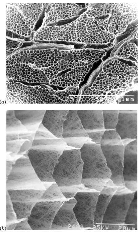
Figure 1-5 - Scanning electron micrograph of the cut surface of bovine sternomandibularis

muscle after digestion with NaOH to remove muscle cell contents and proteoglycans in the IMCT. In (a) we have a low magnification view showing thicker perimysial sheets covering the fascicles along with the thinner endomysial layers; and in (b) a high magnification oblique view showing the fine network of collagen fibres making up the reticular layer of the endomysial sheets that separate adjacent muscles fibres. From (7). ... 1–6

v Figure 1-6 – Light microscopy image of a thin transverse section of SKM tissue revealing:

(a) Interstitial inflammation (H&E x170); and (b) Phagocytosis of degenerating fibers (H&E x170). From (8). ... 1–7

Figure 1-7 - End-stage of disease. Note the massive fat (white cells) and moderate

connective tissue replacement surrounding a cluster of disordered myofibers (dark cells) (H&E x68). From (8). ... 1–8

Figure 1-8 – Light microscopy image of a thin transverse slice of normal SKM tissue. ... 1–8 Figure 1-9 – Example of a cross sectional NMR image of the thigh of a healthy subject.

Muscle tissue, fatty components, fascia and cortical bone may be easily identifiable.

... 1–10 Figure 1-10 – Example of a cross sectional T1-weighted image of the leg of a patient with

necrotizing myopathy showing the resulting fatty infiltration following muscle

degeneration, remarkably on the soleus and gastrocnemius medialis. ... 1–11

Figure 1-11 – T2-weighted image of the thighs with application fat-saturation (STIR).

Inflammation sites are indicated by arrows. Note the hypo-signal from subcutaneous fat and bone marrow because of the application of fat saturation... 1–12

Figure 2-1 – (a) The magnetic dipole moment produced by a dimensionless particle with

an electric charge , inertial angular momentum . (b) Illustration of the precession of the spin magnetic moment around the external magnetic field as a consequence of the torque resulting from their mutual interaction. mass , running within circular trajectory with radius with a linear moment and (Taken from Haacke, Brown,

Thompson, & Venkatesan., 1999). ... 2–2 Figure 2-2 - Illustration of the process of magnetization excitation by the application of an

oscillatory magnetic field perpendicular to , at the Larmor frequency. Note that from a referential rotating at the Larmor frequency the excitation process is seen as a precession of around . ... 2–5

Figure 2-3 - (a) Illustration of the magnetization tipping by the application of a -pulse on

the y-direction, and (b) the independent effects of the 180° and the 90° components on the magnetization. ... 2–6

Figure 2-4 – Illustration of the exponential behaviour of the (a) longitudinal and (b)

transverse relaxation processes. Note in (b) the exponential modulation of the spin-spin relaxation by field inhomogeneities leading to the faster T2* relaxation. ... 2–8

Figure 2-5 – (a) 1H-NMR signal acquired from within a volume containing muscle tissue and subcutaneous fat. (b) The corresponding extracted spectrum resulting from the Fourier transform of the acquired signal. Contributions from lipids were painted in grey. ... 2–9

vi Figure 2-6 – Illustration of the physical interpretation of the Fourier transform of the

signal acquired in the presence of a gradient field. The acquired signal is the inverse Fourier transform of the projection of the spin magnetization on the direction of the gradient. ... 2–11

Figure 2-7 – Illustration of the radial k-space sampling method. (a) Projection of the

magnetization distribution, , on the direction perpendicular to the gradient, . (b) The acquired signal corresponds to a k-space line crossing the origin with inclination determined by . The Fourier transform of the different projections of the spin

magnetization distribution correspond to different lines of its k-space representation. These lines cross the origin and have the same direction than the applied gradient. 2–

12

Figure 2-8 – Schematic illustration of the linear space sampling. Parallel lines of the

k-space are acquired at each readout interval. In order to move from the centre of the k-space to the initial point of each line, the phase of is prepared before readout by application of two orthogonal gradients, say Gx and Gy. Once at the initial point , all the points are registered, with , where “res”

defines the number of points registered per line, which will be directly related to the spatial resolution of the image. ... 2–13

Figure 2-9 - Illustration of re-establishment of phase coherence following the application

of a 180° pulse. represent the instant just after application of the 180° pulse at the time , supposing the effect of the pulse is instantaneous. Note that the individual spin magnetic moments conserve their local precession frequency during all the experiment. Complete refocusing occurs at . ... 2–14

Figure 2-10 - Illustration of the spin echo signal. Note the T2’ recovery following phase

reversal of the FID signal originated from the 90° pulse after application of the 180° pulse. Note also the irreversibility of the T2-decay. (The wiggling inside the T2* envelope is due to off-resonance effects). ... 2–15

Figure 2-11 – Simplified scheme of the gradient and RF-pulse time sequence for the

acquisition of a gradient echo. ... 2–16

Figure 2-12 – Appreciable transverse magnetization generated by a small flip angle,,

which leaves the longitudinal magnetization mostly intact. ... 2–16

Figure 2-13 – (a) Method for observing signal decay from a series of 90°-180°-pulse

experiments with different echo times. (b) Multi spin-echo method for observation of signal decay free of diffusion effects. ... 2–19

Figure 2-14 – The signal evolution in the Carr-Purcell method for different echo-times.

vii

observable to the intrinsic T2. ... 2–20

Figure 2-15 – Schematic illustration of the magnetization vector response to two

consecutive imperfect refocusing pulses in the (a) Carr-Purcell method, and (b) Meiboom-Gill improved method. Observe the accumulation of the flip angle error in the Carr-Purcell method (a). Notice in (b) that the flip angle error, φ, is corrected after the second refocusing pulse. In (b), the 90° component of the first refocusing pulse will tip previously excited transverse magnetization to the longitudinal direction (red vectors). This longitudinally stored magnetization will be re-tipped to the

transverse plane completing its 180° flip by the action of the 90° component of the second refocusing pulse. This magnetization will be refocused leading to the so called stimulated echo at a time with the same phase of the primary echo refocused by the action of the 180° component (blue vectors). ... 2–21

Figure 2-16 – Time sequence diagram of the CPMG technique. A series of equally spaced

180°-pulses is launched after an interval TE/2 from the 90°-pulse. The phase of the 180°-pulses is shifted of 90° from the 90°-pulses so that imperfect refocusing are corrected for the even echoes. ... 2–22

Figure 2-17 – Plots of a standing wave at different times. Note that its amplitude at each

point in space is modulated by a constant value. ... 2–23

Figure 3-1 – (a) presents the theoretical T2-decay of muscle and fatty components. In (b)

T2-weighted images of the thigh acquired at different echo-times, TE=10ms and 160ms (adjusted to the same contrast window level). The contrast between muscle and fatty components depends on the ration of their relative signal intensities which varies in time due to their different T2-values. ... 3–2

Figure 3-2 – Signal amplitude vs. echo-time for a voxel within the muscle. Images of the

lower legs acquired at different echo times with a multi-spin-echo sequence. Note the exponential T2-relaxation behaviour. ... 3–3

Figure 3-3 – Pulse sequence diagram of a (a) CMPG-like MSE sequence and (b) a MSE

sequence with variable crusher gradients for nulling stimulated echo contributions. The RF-pulse time sequence is the same for both methods, except for the phase of the pulses that are only explicit for the CPMG-like MSE sequence (a). Note in (a) that the gradient moments are identic between refocusing pulses by application of the so called phase rewind gradients. ... 3–4

Figure 3-4 – Example of a 1H-NMR spectrum acquired at 3T from a volume containing muscle and subcutaneous fat. Peaks containing contributions exclusively from lipids were painted grey. ... 3–5

viii

selectively excited with a 90°-pulse and spoiler gradients are applied immediately after, in order to null the transverse fat magnetization components. At the end only water longitudinal magnetization components will last, and a imaging sequence may be executed to produce water only images. ... 3–6

Figure 3-6 – (a) Illustration of the idea behind the 2PD method; the phase of fat spin

isochromat is inverted at topp and might be trivially isolated from the water spin

isochromat by simply summing or subtraction both images. (b) Illustration of the idea behind the 3PD method; the local B0-shift may be estimated from the phase

difference between both in-phase images. Note that when in the presence of a B0-shift, although fat and water signal will be in-phase at tin1 and tin2, and in

opposed-phase at topp, they won’t be parallel and antiparallel between images due to the

shifted local precession frequency. ... 3–7

Figure 3-7 – Illustration of fat and tissue water longitudinal magnetization component

recovery during T1-relaxation. In the STIR method, the imaging sequence is executed at the inversion time, TI, where only tissue water has non-zero longitudinal

magnetization. M0w and M0F are the equilibrium fat and tissue water magnetizations. ... 3–9 Figure 3-8 – Schematic illustration of a triglyceride molecule along with a proton (1H)

NMR spectrum of isolated triglyceride molecules extracted at 14 teslas. Triglycerides consist of one glycerol (to the left) and three fatty acids (to the right). In this example, the fatty acids are: palmitic acid (top), oleic acid (middle), and linolenic acid

(bottom). Assignment of the different protons to the resonances A–J is indicated. A virtual water peak is superposed to the spectrum. ... 3–10

Figure 3-9 – Example of ROIs drawn manually to delineate the thigh muscles. ... 3–13 Figure 3-10 - (a) B1+ map (ratio between actual flip angle and the applied one) the area

inside the red contours correspond to B1+ ranging between 85% and 130%. (b) The corresponding muscle water T2-map of a healthy volunteer’s thigh. ... 3–15

Figure 3-11 - Relationship between B1+ map (expressed as a percentage of the actual flip

angle) and water T2-values determined on a group of 20 healthy volunteers. ... 3–17

Figure 3-12 - Box plot of T2-values in voxels with different fat signal fractions calculated

using (a) the tri-exponential model (b) the exponential model. With the mono-exponential model, T2-values were systematically more elevated when fat content was higher. Significant differences in T2-values between normal and abnormal subjects were observed using both models (p<1e-4). ... 3–19

Figure 3-13 – Plots of the water T2-values, as determined with the proposed

ix

fitting against Dixon-based fat fraction. A strong correlation exists between global T2-value and fat content. In contrast, water T2-values derived from the

tri-exponential model were independent from the Dixon fat fraction. Abnormal muscles are also identifiable by elevated global T2-values. ... 3–20

Figure 3-14 - Relationship between fat fractions (F0) extracted from Dixon-based fat

fraction and MSME based fat fraction. Fat fraction (F0) values obtained with both techniques were highly correlated: R²=0.89 with a slope close to unity (0.94). ... 3–21

Figure 4-1 - (a) SSFP signal as a function of and calculated with Bloch simulation

(thin line) or using an approximate analytical model (Eq. 4.2) (thick line). Experimental data (closed circles) acquired in a 0.1 mM MnCl2 phantom were

superimposed on simulated curves. The constant value (dotted line) represents the ideal RF spoiled signal: ( -

) ( -

). Arrows indicate

the largest ( ) for which Eq. 4.2 is still applicable. In (b) the calculated deviation (i.e., the relative difference between derived from Eq.

4.2 and from Bloch simulation) is plotted against for the same and values, as

in (a). Relevant experimental parameters were TR = 5 ms, TE = 3 ms, (20°, 40° and 90°), (1°, 5°, 10°, 15°, 20° and 30°). Common parameters for both

computations in Fig. 1 (Bloch simulation and Eq. 4.2) were TR = 5 ms, (20°, 40° and 90°), to 50°, in 0.25° steps, T1/T2 = 886/86 ≈ 10. ... 4–13 Figure 4-2 – (a) T2estim/T2 ratio as a function of calculated using either numerical

simulation of Eq. 4.4 (open squares) or the analytical function derived from Eq. 4.8 (solid line). To gain insight on the flip angle dependence of T2 estimation, T2estim/T2

ratio was also plotted as function of in (b). Experimental data (closed circles) acquired in a 0.1 mM MnCl2 phantom were superimposed on the simulated curves.

The constant value (dotted line) represents T2estim/T2 = 0.95. Relevant experimental

parameters were TR = 5 ms, (20°, 40°, 60°, 80° and 90°), , . Computational parameters were T1 = 886 ms, T2 = 86 ms, TR = 5 ms, to 90°,

in 5° steps, and . ... 4–14

Figure 4-3 - Impact of inaccuracy of T1 on T2 computation using Eq. 4.9: Numerical

simulations (symbols) and analytical solution (lines) show that the sensitivity of T2 to

T1 errors becomes more important with decreasing FA or T1/T2 ratio. Relevant

computational parameters were: TR = 5 ms, or 80°, , . 4–

15

Figure 4-4 - Flip angle sensitivity in T2-pSSFP mapping: Percent change in T2 derived

x

= 40) as a function of FA deviation. In the presence of inaccurate FA, T2

measurement presents a significant bias which becomes more important with

increasing T1/T2 ratio (solid lines). Accurate T2 quantification is achieved if actual FA

is used in Eqs. 4.4 and 4.9 (dotted lines). Relevant computational parameters were: T1 = 886 ms, T2 = 86 ms, TR = 5 ms, , . ... 4–16 Figure 4-5 - T2-mapping of a liquid phantom at 3T (reference T2 = 86 ms): T2-maps and

respective histograms derived from Eq. 4.4 (a, b), Eqs. 4.4 and 4.9 (direct

approach) (c, d) assuming T1 = 886 ms and from Eqs. 4.13 (iterative approach) (e, f)

assuming T1 = 886 ms and starting T2 = 80 ms. Accurate and precise T2-mapping

was only possible after concomitant T1 and FA corrections for both approaches (d, f).

Relevant experimental parameters were: TR = 5 ms, TE = 3 ms, , ,

. ... 4–17 Figure 4-6 - In vivo skeletal muscle T2-mapping at 3T: T2-maps (axial and sagittal views)

derived from 3D pSSFP scans. Images were acquired in quadriceps muscles of a volunteer, immediately before and on the 1st, 2nd, 3rd and 10th day following an eccentric exercise session. FA deviation maps are also shown to illustrate the B1+

inhomogeneity in the knee coil. Axial views correspond to representative medial and distal sections of the quadriceps muscles and its relative positions are indicated in the anatomical T1 weighted images (black lines). Parametric maps present large areas of

T2 increases at two days post-exercise, corresponding probably to muscle injury. T2

changes were predominantly located in the distal portion of the vastus medialis (VM) muscle and close to the muscle–tendon junction (arrow). Experimental parameters for T2-pSSFP imaging were , and 15°, TR/TE = 6.3/2.8 ms, NEX = 2. All T2-maps were corrected for B1+ inhomogeneity and T1. Overall T2-pSSFP

acquisition time was ~10 min. ... 4–18

Figure 4-7 - Comparison of T2 in quadriceps muscles of a volunteer as measured by

MSME and T2-pSSFP methods: (a) Overall T2 measurements (all days, all slices, all

ROIs) as a function of FA deviation (symbols). Error bars were omitted for the sake of clarity. On average, standard deviation for both methods was ~3 ms. Dashed lines are just guidelines. (b) Bland-Altman plots showing the limits of agreement between T2 as determined by pSSFP (Eq. 4.9) and standard MSME method. The center line

represents the mean differences between the two methods, and the other two lines represent 1.96 SD from the mean. To limit the impact of B1+ inhomogeneity in

Bland-Altman analysis only five slices localized at the center of the transmitter coil were considered. Relevant experimental parameters for MSME scans were: TR = 3 s, 17 echo times (TE) range = 8.1 to 137.7 ms, in-plane resolution = 1.4 x 1.4 mm2, 11

xi

slices, slice thickness = 8 mm, slice gap = 20 mm, acquisition time ~ 5 min. ... 4–19 Figure 4-8 - Axial T2-maps obtained from T2-pSSFP experiments carried out in a

myopathic patient (a) and in a healthy volunteer (c). For comparison, a fat-suppressed T2-weighted image from the same patient is displayed in (b). An FA deviation map measured in the volunteer is also shown to illustrate the asymmetric B1+ inhomogeneity in the thighs (d). Histograms extracted from T2-maps are shown

in (e). A homogeneous distribution of T2-values, centered on 37 ms, is observed for the healthy volunteer (thin line), whereas for the patient (thick line), median T2 is

shifted to 44 ms. Note regions of increased T2 (up to 180 ms) in the patient, reflecting

muscle edema. Experimental pSSFP parameters were: in-plane resolution = 1.4 x 1.4 mm2, slice thickness = 5 mm, 64 slices, , and 15°, TR/TE = 6.3/2.8 ms, NEX =1. Total T2-pSSFP acquisition time was ~3 min. T2-maps were corrected for B1+ inhomogeneities and T1. SNR1 was higher than 50 for all analysed muscles.

Relevant experimental parameters for T2w imaging were: TR = 3 s, TE = 45 ms,

Turbo-factor = 2 ms, in-plane resolution = 1 x 1 mm2, 27 slices, slice thickness = 5 mm, slice gap = 5 mm, acquisition time ~ 5 min. ... 4–20

Figure 5-1- RF-pulse and B0 gradient time sequence diagram representing the

implemented ISIS-CPMG method. In the ISIS module adiabatic inversion pulses are selectively turned on following an 8 steps combination as indicated. Fat saturation is accomplished with a 90° hard pulse with 1.5 ms long 90° hard pulse centred at -432 Hz from water proton frequency, and is launched just after each of the ISIS steps. CPMG pulse train is launched 2 ms after the Fat-Sat module. ... 5–5

Figure 5-2 – (a) plot the x and y components of the designed RF-B1 field wave form and

(b) the simulated 20 mm slice profiles for short and long T2-species. Short T2-species are characterized by T2/T1 = 1/350 ms, and long T2-species were characterized by T2/T1 = 40/1200 ms. ... 5–5

Figure 5-3 – Experimental demonstration of CPMG phase cycling. Plots of echo amplitude

vs. echo-time resulting from two CPMG acquisitions with opposed refocusing pulse phases (red and blue). Note that after summation (black), FID signal contributions cancel out and signal amplitude approaches zero asymptotically. ... 5–6

Figure 5-4 – Picture of a subject’s leg, placed on the inferior half of the transceiver coil,

after step 1 of the vascular draining procedure. Note the cuff wrapped around the thigh. ... 5–7

Figure 5-5 - Protocol timeline for the T2-spectra acquisitions at different vascular filling

conditions: (i) With the patient in « supine, foot first » orientation, and its calf positioned in the transceiver coil, the vascular draining procedure was first applied;

xii

(ii) Localized CPMG signal was acquired with the VOI located within the soleus during 5 min; (iii) Vascular filling step is performed and another CPMG acquisition of 5 min is launched over the same VOI after a 5 min interval; (iv) Pressure is released from the cuff and another CPMG acquisition of 5 min is performed over the same VOI after a 5 min interval. ... 5–8

Figure 5-6 - Illustration of a virtual non-exchanging system that presents T2-relaxation

behaviour identical to that of a real exchanging system. The apparent T2-values and relative fractions characterizing the pseudo compartments of the virtual system are functions of the intrinsic relative fractions, T2-values and exchange rates of the real system. In this case, a tri-compartmental two-exchange system with no direct

exchange between compartments 1 and 3. ... 5–11

Figure 5-7 - (a) Plot of T2-decay curves obtained for a subject under different vascular

filling conditions. The lines passing through the points correspond to the fitted curves resulting from the regularized inversion solution, and (b) presents the corresponding obtained T2-spectra. ... 5–13

Figure 5-8 - Characteristic relaxation curves of the vascular draining (triangles), normal

(squares) and vascular filling (circles) conditions, and the corresponding fitted curves characterized by the extracted intrinsic parameters of the 2SX model for both transcytolemmal (crosses) and transendothelial (lines) exchange regimes. ... 5–15

Figure 5-9 - (a) Characteristic relaxation curves of the vascular draining (triangles),

normal (squares) and vascular filling (circles) conditions, and the corresponding fitted curves (lines) characterized by the extracted intrinsic parameters of the 3S2X model; (b) Obtained T2-spectra from regularized inversion of the fitted curves

resulting from the 3S2X model. ... 5–16

Figure 5-10 - Projection of the VOIs on the sagittal, coronal and axial T1-weighted

FLASH images of the calf of the patients (from left to right). (a) VOI located within the soleus of a patient diagnosed with Charcot-Marie-Tooth disease; (b) and (c) show the VOIs located within the soleus and tibialis anterior of a patient diagnosed with eosinophilic fasciitis, respectively; (d) VOI located within the tibialis anterior of a patient diagnosed with a necrotizing myopathy. ... 5–22

Figure 5-11 – Extracted T2-spectra characterizing each system defined by the intrinsic

parameters presented in Table 5-4, representing respectively: (a) Normal tissue; From (b) to (d) there is progressive increase in interstitial oedema; (e) inflammation, characterized by interstitial oedema and higher perfusion; and (f) is supposed to represent necrotizing tissue, characterized by inflammation with high membrane permeability. T2-spectra are plotted with logarithmically scaled abscise for correct

xiii

visualization of peak area. The T2-value and relative fraction (Eqs. 5.6, 5.7)

characterizing the T2-peaks are indicated in the plots. ... 5–25

Figure 5-12 – T2-decay curves and the T2-spectra obtained for each in vivo data set: (a)

soleus of the patient diagnosed with Charcot-Marie-Tooth disease; (b) soleus and (c) tibialis anterior of the patient diagnosed with Shulman’s syndrome; (d) tibialis anterior of the patient diagnosed with a necrotizing myopathy; and (e) soleus of a healthy subject. T2-spectra are plotted with the abscise in logarithmic scale for correct visualization of peak area. ... 5–28

Figure 6-1 – Comparative morphologic features of SKM histology between control (a) and

Duchenne muscular dystrophy (DMD) cases (b, c). The intracellular matrix occupies a much smaller volume fraction in control (a), resulting in capillary-to-muscle fiber distances which are minimal, in contrast with the dystrophic tissue (b). Collagen I immunostaining highlights the endomysial layers which are abnormally thick in the dystrophic tissue (c). Taken from (141). ... 6–2

Figure 6-2 – The hypo-signal of compact collagenous tissue structures observed in NMR

images. (a) Spin-echo PD image (TE = 9.5 ms) of the thighs. The arrows point to the dark visible fascia with its characteristic hypo-signal. (b) Spin-echo T1-weighted image (TE = 16 ms) of both buttocks. The Arrows point to a dark visible thin fibrotic cord in atrophic right gluteus maximus muscle. Normal left side may be used for comparison. Image in (b) was taken from (144). ... 6–3

Figure 6-3 – Simplified FR-pulse and gradient time sequence for (a) 2D-GRE and (b)

3D-GRE NMRI techniques. For both methods, the phase encoding gradients imposes a minimum dead time in which no signal is acquired. For the 2D case, a slice selection mode is applied which elongates the dead time due to relaxation effects during excitation process. ... 6–4

Figure 6-4 – Schematic illustration of k-space sampling for (a) 3D and (b) 2D radial

acquisition methods. ... 6–5

Figure 6-5 – Principle of half RF-pulse selection for acquisition of short relaxing NMR

signal. Slice profile is completely selected after summation of acquisitions with inverted polarity of selection gradient. ... 6–6

Figure 6-6 - Simplified FR-pulse and gradient time sequence for (a) a 2D-GRE sequence

with half excitation pulse and (b) a 3D-GRE sequence. Radial acquisition allows acquiring data right after the excitation. The dead time is determined by the time it takes for the RF system to change from transmission to acquisition mode, usually on the order of 10 to 100 µs. ... 6–6

xiv

(lateral head), soleus, peroneus longus and tibialis anterior over the central slice. (b) ROIs A and B delimiting fascia and aponevroses between the gastrocnemius and the soleus; ROI-B was traced in order to include adjacent muscle structures. ... 6–8

Figure 6-8 – Logarithmic plot of the time evolution of the signal amplitude obtained from

the ROIs traced in the gastrocnemius lateral (a), gastrocnemius medial (b), peroneus longus (c), soleus (d) and tibialis anterior (e), along with the corresponding fitted curves. ... 6–9

Figure 6-9 - Logarithmic plot of the time evolution of the signal amplitude obtained from

the ROI-A delimiting the fascia between the soleus and the gastrocnemius and the enlarged ROI-B including adjacent muscle tissue, along with the corresponding fitted curves. ... 6–10

Figure 6-10 – NMRI of an axial slice of the calf of a healthy volunteer using a 2D-UTE

sequence with an echo-time of 0.2 ms, TR = 30 ms and FA = 5°. Note that structures with elevated relative fraction of short-T2-components such as fascia and cortical bone still present smaller signal intensity. However, cortical bone presents higher contrast with other tissue structures due to the high relative fraction of its short-T2-components and to the very short T2-value that characterizes them. ... 6–12

Figure 6-11 – Plot of amplitude modulation of the theoretical fat signal as a function of

time for the fat model given in Table 6-3. Two fat signals were simulated; one in which no T2-relaxation was considered (blue) and a second inserting the T2 of each individual hydrogen group of the lipid molecule. Note that the impact of the phase shift accumulation between the different hydrogen groups in the amplitude

modulation is much more important than the T2-relaxation effects. ... 6–13

Figure 6-12 - image resulting from the subtraction of an UTE image acquired at 2.5 ms

from another UTE image acquired at 0.2 ms (see Figure 6-10).Note the high residual signal from short-T2 structures such as cortical bone and fascia. Notice also the important residual signal on the subcutaneous fat. ... 6–16

Figure 6-13 – Extracted Short T2-map fraction, using the dual-echo method with

correction for T2* of long T2-components and fat signal contributions. ... 6–19

Figure 6-14 – Histogram of the relative fraction, Sf, of signal from short-T2 for pixels with . ... 6–20 Figure 6-15 - Sensitivity profiles of the short-T2-imaging technique describe in Eq. 6.12 to

tissues with different short T2-values (1 µs to 10ms ) for different minimum echo-times (10, 50 and 200 µs). The horizontal dashed line represents the limit of 20% contribution from a short-T2-component. Note that the T2 of maximum sensitivity decreases with the minimum echo time, along with the minimum T2 whose

xv

xvi

List of Tables

Table 3-1 - Spectral model of the fat resulting from spectroscopy data. For each peak were

reported: the relative shifts to the water, the T2-relaxation time and the relative amplitude with respect to the fat component of the voxel. ... 3–14

Table 3-2 - Mean (Eq. 3.3) and mean squared deviation with respect to a reference value

(33.9 ms) of water T2 (Eq. 3.4), with respect to different B1+ range as well as the fraction of muscle voxels that are in the specified B1+ range with the respect to the total number of voxels. ... 3–18

Table 4-1 - Typical values for ξ(α), which must be determined numerically, for different

flip angles, α. ... 4–4

Table 5-1 - Results obtained from the mono- and biexponential fits and regularized

Laplace inversions for the relative fractions and corresponding T2-values, by means of mean(SD), between subjects for each vascular filling condition. ... 5–14

Table 5-2 - Extracted intrinsic parameters of the 2SX model for the three vascular filling

conditions at transcytolemmal and transendothelial exchange regimes; SE is

presented within brackets. ... 5–14

Table 5-3 - Extracted intrinsic parameters of the 3S2X system characterizing the

intracellular, interstitial and vascular spaces for the three vascular filling conditions; SE is presented within brackets. ... 5–15

Table 5-4 – Intrinsic parameters characterizing the simulated systems modelled in order to

represent oedematous, inflamed and necrotizing tissue. ... 5–20

Table 6-1 - Results for the extracted mean relative fraction and T2*-value of the short

component, and the T2*-value of the long component for the ROIs traced in the muscles (see Figure 6-7 a) and for the ROIs A and B traced around the fascia (see Figure 6-7 b). Results are presented as mean(SD) for the muscles and as mean(SE) for each ROI around the fascia. ... 6–10

Table 6-2 – Observed T2* values of some tissue structures at 3 T. ... 6–11 Table 6-3 – Relative fraction and Larmor precession frequency of the different peaks in the

1–1

CHAPTER 1

General Introduction

In recent years Nuclear Magnetic Resonance (NMR) techniques have demonstrated their significant importance in the field of neuromuscular diseases (NMD), getting increasing attention from the scientific community for their potential applications as non-invasive monitoring and investigative tools. The present work consisted on the adaptation of proof of concepts into clinically applicable research tools for characterization of skeletal muscle (SKM) tissue, with the objective of contributing to the consolidation of quantitative NMR tools for studying muscle pathology.

In this chapter, we shall recall the macroscopic and histological architecture of the normal SKM tissue and the most common alterations observed in NMD. The main current NMR clinical tools to characterize these alterations are introduced. We shall discuss their current limitations and the potential applications that shall outcome from their optimization and further development, highlighting the current need for quantitative tools in clinical research.

Finally the limitations of the clinical application of the currently available quantitative NMR tools are discussed, and we describe how the methods that were applied and explored in the present work to expand these limits are organized in this manuscript.

1.1. Skeletal muscle structure and histology

1.1.1. Striated muscle architecture

Muscle tissues are structurally classified as: smooth, mostly found in the walls of digestive organs, uterus and blood vessels; cardiac, found only in the heart; and skeletal, attached to bones by bundles of collagen fibers known as tendons and are responsible for skeletal movement and posture maintenance.

Skeletal muscle is designed as a bundle within a bundle arrangement (Figure 1-1). The entire muscle is surrounded by a connective tissue layer called epimysium and is made up of multiple smaller bundles containing hundreds (100-200) of muscle cells (myofibers)

1–2 called fascicles. The fascicles are held together by a thinner layer of connective tissue called perimysium which provides pathway to the major blood vessels as well as arterioles, venules and nerves through the muscle. Each muscle cell in a fascicle is surrounded by an even thinner connective tissue sheath known as the endomysium which is the pathway for capillaries. The connective tissue covering gives support and protection to the myofibers, allows them to withstand the forces of contraction and plays an important role in the force transmission between muscles and from muscles to tendons and bones.

Figure 1-1 - Structural organization of the skeletal muscle as a bundle within a bundle

arrangement. From the muscle fibers to the fascicles grouped to form the entire muscle.

[Copyright © 2011 Pearson Education, Inc., publishing as Benjamin Cummings,

http://classconnection.s3.amazonaws.com/811/flashcards/141811/jpg/fascia1320418174703.jpg]

Water makes up approximately 76% of muscle tissue weight (1), and is distributed within intracellular, interstitial and vascular spaces, with corresponding average relative fractions of approximately 85, 10 and 5%, respectively (Robertson 1961; Ling & Kromash 1967; Neville & White 1979).

1.1.2. Muscle cell (Myofiber)

Myofibers are long cylindrical multinucleated cells that run along the entire length of the muscles. Figure 1-2 illustrates their intracellular organization. The nuclei are located at the periphery just beneath the sarcolemma (cell membrane) and the cell is densely packed

1–3 with hundreds to thousands of myofibrils, which consist of compactly packed cylindrical bundles of contractile myofilaments, disposed parallel to each other and to the axis of the cell.

Figure 1-2 – Illustration of a skeletal muscle cell (myofiber). Note the tubular system of

sarcolemma invaginations (T-tubules) that are linked to the tubules of the sarcoplasmic reticulum that surround each myofibril. The T-tubules are interconnected and opened to the interstitial space, giving the cell a cylindrical spongy-like structure. The small relative volume left in the sarcoplasm is packed with mitochondria (subsarcolemmal and intermyofibrillar), vesicles, lysosomes, lipid droplets among other cellular structures.

[Found at: http://classes.midlandstech.edu/,

http://classes.midlandstech.edu/carterp/Courses/bio210/chap09/lecture1.html]

The reduced space left in the cytoplasm (sarcoplasm) is packed with mitochondria (subsarcolemmal and intermyofibrillar), vesicles, lysosomes, lipid droplets, glycogen granules among other cellular structures.

Myofibrils are composed of repeating sections of sarcomeres, which are mainly composed of two long fibrous proteins; actin and myosin (see Figure 1-3). These proteins are arranged parallel to each other in a cylindrical structure, with each myosin filament usually surrounded by 6 actin filaments.

1–4

Figure 1-3 - Sarcomere consisting on a bundle of thin and thick myofilaments made up of

protein molecules called actin and myosin, respectively. These proteins are arranged parallel to each other in a cylindrical structure, with usually six actin filaments surrounding one myosin filament. Actin molecules are attached the z-discs, which are constituents of the cytoskeleton and define the boundaries of a sarcomere unit.

[Copyright © 2009 Pearson Education, Inc., publishing as Benjamin Cummings,

http://classes.midlandstech.edu/carterp/Courses/bio210/chap09/lecture1.html]

Figure 1-4 presents a transmission electron microscope image of a longitudinal section cut through an area of human skeletal muscle tissue, where it is possible to identify each sarcomere unit, whose schematic illustration is presented in Figure 1-3.

Figure 1-4 - Transmission electron microscope image of a longitudinal section cut

through an area of human skeletal muscle tissue; borders of two cells separated by the endomysium. Image shows several myofibrils, each with the distinct banding pattern of individual sarcomeres: the darker bands are called A bands(the A band includes a lighter central zone, called the H band), and the lighter bands are called I bands. Each I band is bisected by a dark transverse line called the Z-line). Paired mitochondria (white arrows pointing to some of them) are on either side of the electron opaque Z-line. The Z-Line marks the longitudinal extent of a sarcomere unit.

[Found at: http://remf.dartmouth.edu/, http://remf.dartmouth.edu/images/humanMuscleTEM/source/2.html, by Louisa Howard]

1–5 The myofibrils occupy approximately 80-90% of the myofiber volume (4). In humans, the cross-sectional diameter of muscle fibers varies with age; sizes remain relatively constant in adulthood and tend to decline with old age. The average diameter of a myofiber in adults is around 50-80µm, while the diameter of a myofibril is around 1µm.

Myofibers may be differentiated by their metabolic and functional characteristics (i.e., oxidative vs. glycolytic, fast vs. slow twitch (contraction) ). These differences reflect histochemical and physiological variations between myofibers, such as: number of mitochondria, content of myoglobin, capillary density, lipid and glycogen storage, etc. These differences lead to the classification of myofibers into: type-1, which present slow twitch, predominant oxidative metabolism and high resistance to fatigue; type-2B, which present fast twitch, predominant glycolytic metabolism and low resistance to fatigue; and type-2A, which presents a fast twitch, high glycolytic and oxidative metabolism and higher resistance to fatigue then type-2B fibers.

In average, fiber types are approximately evenly distributed within muscles. Variations on their relative fractions reflect muscle activity and function, and have been shown to change as a response to specific training (5).

1.1.3. Intramuscular connective tissue: epimysium, perimysium

and endomysium.

Intramuscular connective tissue (IMCT) is principally composed of fibers of the proteins collagen and elastin, surrounded by a proteoglycan (PG) matrix. The collagen and elastin contents as percentage of dry tissue weight are 1-10% and less than 0.1-2% respectively, varying with age and muscle(6). Within the anatomical relevant structures of the IMCT, besides the endomysial, perimysial and epimysial layers, is the basal lamina, a thin connective tissue sheet linking the fibrous (reticular) layer of the endomysium to the sarcolemma. Between the sarcolemma and the basal lamina there are small mononuclear cells called satellite cells, which play a fundamental role in myofiber regeneration.

The proteins and macromolecules forming the IMCT are immersed in the so called interstitial fluid, which is composed of water, salts and plasma proteins. Figure 1-5 presents electron micrograph images of the cut surface of bovine sternomandibularis muscle after digestion with NaOH to remove muscle cell contents and proteoglycans, leaving the perimysial and endomysial layers of the IMCT clearly visible.

1–6 (a)

(b)

Figure 1-5 - Scanning electron micrograph of the cut surface of bovine

sternomandibularis muscle after digestion with NaOH to remove muscle cell contents and proteoglycans in the IMCT. In (a) we have a low magnification view showing thicker perimysial sheets covering the fascicles along with the thinner endomysial layers; and in

(b) a high magnification oblique view showing the fine network of collagen fibres making

up the reticular layer of the endomysial sheets that separate adjacent muscles fibres. From

(7).

1.1.4. Structural and histological alterations induced by

pathology in the skeletal muscle tissue

1–7 alterations that are commonly observed in NMD, and that are expected to appreciably impact proton (1H) NMR observations, without getting into the details concerning the disease-specific mechanisms underlying such alterations.

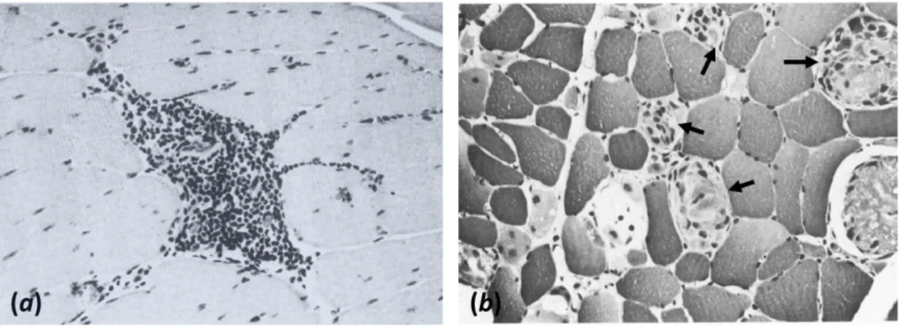
Neuromuscular disorders encompass a large number of diseases that impair the functioning of muscles. An important consequence of the disease activity common to most NMDs is injury at the cellular level. The term cell injury refers to the destruction of the integrity of the sarcolemma, which results in an outflow of cellular organelles into the interstitial space leading to myofiber necrosis. Local inflammation takes place as a response to the degeneration of the cell(s) resulting in interstitial oedema and phagocytosis Figure 1-6.

Figure 1-6 – Light microscopy image of a thin transverse section of SKM tissue revealing:

(a) Interstitial inflammation (H&E x170); and (b) Phagocytosis of degenerating fibers (arrows) (H&E x170). From (8).

Sarcolemma disruption and inflammation are hypothesised to activate the satellite cells that proliferate and differentiate, mostly into myocytes that will fuse with one another or with the myofiber end-fragments to regenerate the injured cell, but also into myofibroblasts that fuse together to form fibrous connective tissue. However, the continuous degeneration processes that take place in some NMD, e.g. Duchenne muscular dystrophy, result in persistent inflammatory response. Although the etiology and pathophysiology of fibrosis is still investigated and debated, it is becoming widely accepted that this chronic nature of the inflammatory response is a key driver of the fibrotic response (9–11), by inhibiting myofiber regeneration and promoting the formation of fibrotic tissue. As a consequence, the disease activity may lead to progressive enlargement of the endomysium and, eventually, complete myofiber replacement by fibrous connective tissue, usually referred to as fibrosis.

The continuous tissue degeneration is followed by ingrowth of fat and connective tissue, and muscle biopsies at advanced stages of disease often reveal important or

1–8 complete myofiber replacement by fat and fibrosis (Figure 1-7).

Figure 1-7 - End-stage of disease. Note the massive fat (white cells) and moderate

connective tissue replacement surrounding a cluster of disordered myofibers (dark cells) (H&E x68). From (8).

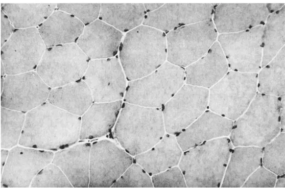
As in comparison to normal skeletal tissue (Figure 1-8), the above discussed alterations share the common features of altered water content and distribution within tissue compartments, and increased content of intramuscular fat and fibrosis.

1–9

1.2. The role of NMR in myology clinical research

The continuous advances of NMR techniques, especially the recent progress on the development and optimization of quantitative examination tools, have driven increased attention to Nuclear Magnetic Resonance Imaging (NMRI) and Nuclear Magnetic Resonance Spectroscopy (NMRS) and extended their applications in the neuromuscular field, from supplementary diagnostic tools to quantitative non-invasive outcome measures in clinical studies.

Muscle NMRI is sensitive to pathology induced changes such as fat degeneration and inflammation, and has been proven capable of revealing disease-specific patterns of selective muscle involvement (12–16), lending itself well for guiding genetic tests and for optimal muscle selection for biopsy (17), improving the diagnostic workup (18). Furthermore, progressive characterization of such patterns shall help to better understand the pathogenesis of neuromuscular disease.

Quantitative NMR methods have provided non-invasive outcome measures for NMD, offering the possibility of realising longitudinal studies for the follow-up of therapeutic trials and disease progression (19–24), which was just not feasible with purely qualitative techniques, incapable of detecting short duration changes in slow progressing diseases. Moreover, detailed description of disease progression may elucidate still unknown aspects of onset and progression of pathology.

Besides NMRI, Nuclear Magnetic Resonance Spectroscopy (NMRS) techniques have also demonstrated their utility in the clinical field of NMD, as it is a consolidated non-invasive tool for quantifying pathology induced metabolic alterations (25, 26). With correct manipulation, NMR techniques can be made sensitive to different tissue-characteristic physical properties and physiological processes, making it an important investigative tool for studying the physiological mechanisms underlying disease activity.

1.2.1. NMR outcome measures currently available for skeletal

muscle studies

An adult human body is mainly composed of water (60-70 %), proteins (15-25 %) and lipids (5-15%), and these components are distributed at different relative fractions within each type of tissue in the body. Hydrogen nuclei are present in all molecules forming these components and are the most abundant atoms in the human body, which makes it them nuclei of choice for most NMRI applications. In practice, the signal from hydrogen (proton) in proteins is not observable with usual NMRI techniques due to its extremely short T2-relaxation time (T2) (~ 10 µs) (see 2.4), so that most of the signal that is processed in 1H-NMRI techniques comes only from protons in water and lipids.

1–10 The relaxation of water in tissue is very different from the relaxation of pure water, and is usually dominated by the interactions of the water molecules with the macromolecules constituting the tissue. As a consequence, there will be three independent sources of contrast in magnetic resonance images: (i) the volumetric density of detectable protons; (ii) the different intrinsic NMR parameters characterizing water and lipids; and (iii) the different tissue-characteristic NMR parameters of water protons, which are determined by the chemical composition and structure of the tissue.

The different tissues or structures that are identified in standard clinical NMRI of SKM are: muscle, fat, fascia and cortical bone (Figure 1-9); the two last being recognizable by a characteristic lack of signal.

Figure 1-9 – Example of a cross sectional NMR T1-weighted image of the forearm of a

healthy subject. Muscle tissue, fatty components, fascia and cortical bone may be easily identified.

The main explored NMR parameters in current SKM studies are: the chemical shift (see 2.5), which quantifies the different precession frequencies of the magnetization from protons in water and lipid molecules (see 2.5), and is explored to produce separate images of these compounds; and the relaxation times T1 and T2, which are defined in 2.4. NMRI techniques may be specifically adjusted in such a way that the acquired signal will selectively depend mostly on either T1 or T2, and the corresponding image will be referred to as T1- or T2-weighted, respectively, with their contrast determined by the specific relaxation time differences between tissues. As tissue relaxation and composition is usually altered by disease activity, NMRI techniques can be made sensitive to pathology induced tissue alterations such as oedema, inflammation, necrosis, fat infiltration and fibrosis. However, qualitative approaches, such as T1- and T2-weighted imaging, for

1–11 assessing such tissue alterations lack of specificity and are subjective, depending on visual identification of contrast differences. Furthermore, image intensity will be influenced by tissue-independent factors such as technical imperfections of the imaging system. These issues impose the necessity of developing quantitative methods that might offer objective biomarkers for precise characterization of tissue alterations.

Signal detection from thick connective tissue layers or cords such as fascia and fibrosis is a rather complicated issue; some of the NMR parameters of water molecules within the dense collagen matrix of these structures are altered and are only visible with special techniques which have been explored in the present work and will be discussed in details on chapter 6.

Muscle atrophy may be investigated by muscle volumetry, which may be easily obtained after individual muscle segmentation form NMR images. Fat degeneration may be identified in T1-weighted images (see Figure 1-10) and chemical shift-based quantitative NMRI (qNMRI) approaches for quantification of fat infiltration are in relatively advanced stage of development. Furthermore, fat infiltration has already been shown to serve as an outcome measure for characterizing disease progression in some pathologies (20, 21).

Figure 1-10 – Example of a cross sectional T1-weighted image of the leg of a patient with

necrotizing myopathy showing the resulting fatty infiltration following muscle degeneration, remarkably on the soleus and gastrocnemius medial head.

Although more easily detected and quantified, fat infiltration reflects advanced states of pathology, and are particularly useful for characterizing further disease progression and for pattern recognition, improving later diagnosis workflow. On the other hand, inflammation is an indicative of disease activity and could probably be used to detect early

1–12 stages of diseases. However, quantifying inflammation is a rather complicated issue. Inflammation and fat are highlighted in T2-weighted images and it is impossible to distinguish inflamed from moderately fat infiltrated muscle with such contrast. An alternative to distinguish between fat infiltration and inflammation is the application of the so called spectrally selective excitation or fat suppression techniques (see 3.2), resulting in theoretically water only images (see Figure 1-11). Still the detection of inflammation sites in such images is limited by the contrast between inflamed and non-inflamed muscles, which is by itself very sensitive to signal in-homogeneity caused by system imperfections. Furthermore, it is important to realize that sensitivity to progression of pathology or response to treatment relies on the detection of small changes in the explored NMR parameters, which demands the application precise quantitative methods. The solution to overcome the difficulties associated with the characterization of inflammation sites relies on the actual measurement of the relaxation time T2, which has been shown to be abnormally elevated in presence of inflammation.

Figure 1-11 – T2-weighted image of the thighs with application fat-saturation (STIR).

Inflammation sites are indicated by arrows. Note the hypo-signal from subcutaneous fat and bone marrow because of the application of fat saturation.

Quantitative NMRI methods have been and are still being developed, and some clinical studies have already revealed their potential to offer outcome measures of disease progression (20, 21, 24) and the effects of treatment (22, 27). However, these trials also pointed out the precision limitations of the currently available quantitative approaches for the characterization of inflammation, which may result in similar lack of sensitivity depending on the applied methodology.

1–13 physiological alterations, such as necrosis, intracellular or/and interstitial oedema, which may all occur separately or at the same time in some pathological scenarios. These features are responsible for the lack of specificity of T2 on the characterization of pathophysiological processes responsible for the disease progression.

In this work we present, in a first moment, two different methodologies that allow extracting muscle T2-value free of confounding fat signal contributions. Secondly, we present a technique to access information about water distribution within tissue (intracellular, interstitial and vascular), which is presented as a promising solution for addressing the sensitivity and specificity problem related with the observation of muscle T2. Finally, we describe our attempts to detect initial fibrotic tissue accumulation by exploring an especial imaging technique that allows signal acquisition from structures with very short T2-values.

1.3. Thesis overview and contributions

In this section we explain the organisation of the thesis manuscript. In chapter 2 we briefly present the basic physical principles underlying the NMR phenomena, and the resulting properties underlying the contrast mechanisms on NMRI techniques introduced in 1.2.

In chapter 3, we describe a methodology for the quantification of myowater T2-value on NMR images. In contrast to T2-weighted images, this technique allows the extraction of so called T2-maps, which are images of the actual T2-value distribution. This technique characterizes muscle tissue oedema, lesions and damages, by T2 quantification, and simultaneously also the degree of local fat infiltration, which make of it an interesting tool to study inflammation in fat infiltrated muscles. This technique was validated in vivo in healthy volunteers and myopathic patients. The study presented in this chapter was published in the Journal of Magnetic Resonance Imaging (Azzabou et al. 2014, Validation

of a generic approach to muscle water T2 determination in fat-infiltrated skeletal muscle).

In chapter 4, we describe in details the application of another NMRI technique for the extraction of T2-maps. In contrast to the method proposed in Ch. 3, in this technique only water magnetization is selected, allowing simpler post processing. The proposed method also offers simpler approaches for correcting errors caused by system imperfections. This technique was validated in vivo, and the results presented in this chapter were the object of an article published in the journal Magnetic Resonance in Medicine (de Sousa et al. 2012.

Factors controlling T2-mapping from partially spoiled SSFP sequence: optimization for skeletal muscle characterization).

1–14 and the specificity of T2-measurement are approached. The theory of relaxation in tissue is briefly reviewed along with the resulting hypotheses concerning the interpretation of muscle T2-relaxation data. We detail the implementation of a clinical protocol, from the acquisition technique to the post-processing, which allowed us to demonstrate the feasibility of quantifying myowater distribution within intracellular, interstitial and vascular spaces. We also validated a theoretical compartmental exchange model capable of predicting T2-relaxation data in healthy SKM tissue. These results are the object of two international communications (Araujo et al. 2013; Araujo et al. 2014) and an article published in the Biophysical Journal (Araujo et al. 2014. New Insights on skeletal muscle

tissue compartments revealed by T2 NMR relaxometry). Finally, we further developed the

validated compartmental exchange model in order to represent expected tissue alterations, such as cellular oedema, inflammation and necrosis, characteristics of many NMDs. Simulated data from such altered models were analysed with the aim of getting some insight about the potential applications of the developed methodology for studying muscle pathology, and were compared with in-vivo data obtained in patients with NMD.

In chapter 6 we describe the application of an NMRI technique which allows the detection of signal from fast relaxing tissue structures such as fascia, cortical bone and as recently verified (33) fibrosis, for imaging IMCT. First, we describe a study in which we demonstrated the feasibility of detecting a short-T2-component (T2 < 1 ms) in SKM, and collected indices suggesting that it shall represent connective tissue. The results of this first study were communicated in two international conferences, including an oral presentation (Araujo et al. 2011, 2012). Then we proposed and validated in-vivo a post-processing method for imaging the short-T2-components observed in SKM.

Chapter 7 resumes the conclusions from all the obtained results and presents the perspectives for future developmental work, from the application of clinical protocols to the implementation of more sophisticated techniques to complement and extend the limits of application of the methodologies developed and applied in this thesis work.

2–1

CHAPTER 2

Basic Concepts of Nuclear Magnetic

Resonance

In the early 1920’s elemental particles (atomic nuclei, electrons, etc.) have been shown to possess a fundamental property, other than mass and electric charge, called spin. The spin may be seen as the intrinsic angular momentum of elemental particles. Analogously to the magnetic moment associated to the orbital kinetic moment of a particle, we associate a spin magnetic moment to every elemental particle. This intrinsic magnetic property was investigated by studying the interactions of spin with magnetic fields. These studies, first piloted by Rabi and coworkers in the early 1930’s, have shown that, when immersed in an external magnetic field, some atomic nuclei are capable of absorbing and emitting photons (classically, electromagnetic waves) at specific frequencies that univocally identify each element. Their work established the basis for the understanding of the interactions between spin magnetic moments and magnetic fields. These works were further explored by the research groups leaded by Felix Bloch and Edward Mills Purcell that were awarded the 1952 Nobel Prize for “their development of new ways and methods for nuclear magnetic precision measurements”. Their works described the time evolution of the electromagnetic signal in NMR experiments and constitute the basis for the development of NMRI.

The techniques that apply the NMR phenomenon to study a given physical system consist of at least three basic steps:

i- Polarization of the spin magnetic momenta of the system by application of an external magnetic field.

ii- Excitation of the system by absorption of specific frequency selective electromagnetic radiation.

iii- Detection of the electromagnetic signal during the relaxation of the system from the excited to the minimum potential energy state (thermal equilibrium).

The combination of specific and precisely controlled excitation and detection techniques allows one to extract different physical information about the studied system, and still