Uncertainty quantification of the fast flux calculation for a PWR vessel

(1)

HAL Id: tel-02555329

https://tel.archives-ouvertes.fr/tel-02555329

Submitted on 27 Apr 2020

HAL is a multi-disciplinary open access

archive for the deposit and dissemination of sci-entific research documents, whether they are pub-lished or not. The documents may come from teaching and research institutions in France or abroad, or from public or private research centers.

L’archive ouverte pluridisciplinaire HAL, est destinée au dépôt et à la diffusion de documents scientifiques de niveau recherche, publiés ou non, émanant des établissements d’enseignement et de recherche français ou étrangers, des laboratoires publics ou privés.

Uncertainty quantification of the fast flux calculation for

a PWR vessel

Laura Clouvel

To cite this version:

Laura Clouvel. Uncertainty quantification of the fast flux calculation for a PWR vessel. Data Anal-ysis, Statistics and Probability [physics.data-an]. Université Paris-Saclay, 2019. English. �NNT : 2019SACLS414�. �tel-02555329�

(2)

de

doctor

at

NNT

:2019SA

CLS414

Uncertainty quantiﬁcation of the fast ﬂux

calculation for a PWR vessel

Thèse de doctorat de l’Université Paris-Saclay préparée à l’Université Paris-Sud Ecole doctorale n◦_{576 Particules, Hadrons, Énergie, Noyau, Instrumentation, Imagerie,}

Cosmos et Simulation (PHENIICS)

Spécialité de doctorat : Énergie nucléaire

Thèse présentée et soutenue à Saclay, le 13 Novembre 2019, par

L

AURA

C

LOUVEL

Composition du Jury : Pierre D´esesquelles

Professeur des universités, Université Paris-Sud Président Ivo-Alexander Kodeli

Enseignant-chercheur, Institut Joˇzef Stefan, Slovenia Rapporteur Bertrand Iooss

Chercheur Senior, EDF R&D /D´epartement PRISME Rapporteur Claire Vaglio-Gaudard

Chercheur Expert, CEA-Cadarache/DEN Examinateur

Pietro Mosca

Ing´enieur-chercheur, CEA-Saclay/DEN Superviseur

Jean-Marc Martinez

Chercheur Expert, CEA-Saclay/DEN Directeur de th`ese

St´ephane Bourganel

(3)

(4)

Acknowledgements - Remerciements

Je tiens tout d’abord à remercier très chaleureusement mon directeur de thèse Jean-Marc Mar-tinez et mon encadrant Pietro Mosca, sans qui cette thèse n’aurait pas été aussi formatrice. Je vous remercie pour votre gentillesse, votre patience et votre disponibilité. J’ai appris beaucoup à vos côtés. Je suis très reconnaissante de tout ce que vous m’avez enseigné et du temps que vous m’avez accordé.

Un grand merci également aux membres du jury d’avoir évalué mon travail de thèse: le Professeur Pierre Desesquelles pour en avoir accepté la présidence, le Docteur Claire Vaglio-Gaudard pour avoir accepté d’examiner ce travail, et enﬁn le Docteur Ivo Kodeli et le Docteur Bertrand Iooss pour avoir pris le temps de lire ma thèse et d’avoir apporté les remarques et les corrections nécessaires.

L’aboutissement de cette thèse, je le dois aussi à tous.tes ceux.elles qui m’ont apporté leurs aides : Florent Chevallier, Fadhel Malouch, Claude Mounier, Frédéric Moreau, Fabrice Gaudier, Sébastien Lahaye, Stéphane Bourgagnel, Baptiste Broto, Anne-Marie-Baudron, Jean-Jacques Lautard. Merci de m’avoir donné les moyens de réaliser ce travail de recherche. J’ai apprécié de travailler à vos côtés tant sur le plan scientiﬁque que sur le plan humain.

Michel et Pierre, un grand merci à vous deux. Vous m’avez fait conﬁance en me proposant respectivement un stage en Master 1 et 2. C’est quelque part grâce à vous que j’ai découvert mon goût pour la recherche, et que j’ai eu envie de faire cette thèse.

Un petit mot aussi à tous.tes les membres du Service d’Étude des Réacteurs et des Mathé-matiques appliquées (SERMA) du CEA, que j’ai pu côtoyer tout au long de cette thèse. Merci pour votre bonne humeur et toutes les discussions passionnantes partagées ensemble. Agathe, Andréa, Ansar, Brigitte, Carole, Elsa, Emiliano, Eve, Fatima, Igor, Jocelyne, Laurence, Meilin, Mireille, Nicolas, Pierre, Simone, Tan-Dat, Zarko, je vous souhaite le meilleur pour la suite.

Un grand merci aux nombreux.ses doctorant.e.s, postdoctorant.e.s et stagiaires du SERMA: Laurent, Henri, Margaux, Thomas, Wesley, Esteban, Gregory, Michel, Léandre, Soﬁane, Valentin, Paul, Antonio, Dominique, Paolo, Vito, Andréa, Walid. Merci pour tous nos échanges, nos repas et nos pauses café partagés chaque jour, ou presque, pendant plus de trois ans. Vous avez fait de cette thèse un très beau souvenir !

Ami.es d’une vie, de lycée, de classes préparatoires et d’école d’ingénieur . . . Benoit, Bérénice, Blandine, Bruce, Chacha, Cindy, Clément, Clotilde, Cycy, Laura, Lauralee, Lauri-ane, Laetitia, Lise, Ikram, Julie, Maeva, Manuela, Marc, Marie, Nicolas, Petit Soleil, Marion,

(5)

n’a pas de frontière quand le cœur et l’esprit ne connaissent aucune limite. Anne-Marie, Fedo, Florine, Guash, Houda, Isabelle, Issouf, Juliette, Marie-Aimée, Mogahd, Momo, Nina, Shikhali, merci pour votre générosité !

Une pensée particulière également pour ceux qui ont partagé ma vie ces trois dernières années. Bruno, merci pour ta présence pendant ces longues années d’études. J’ai eu de la chance de t’avoir à mes côtés pendant toutes ces années. Merci pour ta gentillesse et ton ouverture d’esprit.

Ma chère Juliette, je tenais aussi à te remercier spécialement. On en a passé du temps ensemble ces trois dernières années... Je crois que si je devais résumer tout ce dont j’ai appris humainement à tes côtés ces dernières années, je serais incapable de l’écrire dans les 175 pages de ce manuscrit. Merci inﬁniment pour tous ces projets menés ensemble !

Nina, merci d’avoir partagé avec moi ces derniers mois de rédaction de manuscrit à la BNF de recherche. Merci pour toutes ces discussions inspirantes. Et surtout merci d’avoir amené un grain de philosophie et de citations d’Hannah Arendt dans cette période qui s’annonçait pourtant diﬃcile. Je suis très ﬁère de te compter parmi mes ami.es et d’avoir partagé tous ces moments avec toi.

Mogahd, je crois que j’ai rarement rencontré de personnes aussi courageuses que toi. Merci pour ta sagesse et pour tout ce que tu m’as enseigné et donné pendant ces deux très belles années. Juliette, Amandine, Alex, Vlad, Daniele, Antonio, Enrica, Alexia, Michel, Moussa, Docta, Domino, Nat & Asha, merci d’avoir été là dans les bons et les mauvais moments. Vous êtes de super colocs !

Enﬁn, Steven merci pour ton soutien sans failles dans la dernière ligne droite de ma thèse, pour ta présence, pour ta patience, pour tes encouragements et pour tes nombreux conseils.

Mes derniers remerciements vont à ma petite sœur, à mes grands-parents et à mes parents qui ont cru en moi et qui m’ont toujours soutenu pendant toutes ces années d’études. Merci pour l’amour que vous m’avez donné.

(6)

(7)

(8)

The production of electricity in Pressurized Water Reactors (PWR), consists in harnessing the heat released from the fission of atoms produced in the fuel of the reactor core, by using water as a coolant. The fission reaction results from the absorption of slow neutrons by nuclei of high atomic number. The nucleus splits into two lighter nuclei, called fission fragments and produces an average of 2.5 neutrons. In order to slow down the high-energy neutrons liberated by the fission reaction, the water also plays the role of moderator. A reflector is then installed around the reactor core to reduce neutron leakage by scattering back those which have escaped from the core. Despite the presence of the reflector, some neutrons still reach the reactor pressure vessel. The issue is that intense irradiation can alter the vessel microstructure and have an unfavourable effect on mechanical properties. This phenomenon is one of the major limiting factors to nuclear reactor lifetime. The vessel, which cannot be replaced, is actually the second barrier against the radioactive leakage. Surveillance programmes are therefore necessary for safety assessment and for verifying the vessel structural integrity (Steele,1983).

Core Baﬄe

Vessel Core Barrel

Fuel assembly Thermal shield

Capsules

Specimens

Dosimeters

ΔRTndt= f (φ1MeV)

Fast ﬂuence φ1MeV

Calculation

Prediction Figure 1: General Methodology in Irradiation Surveillance Programmes

Two tracks are commonly adopted to monitor the eﬀects of neutron irradiation on the re-actor vessel under actual operating conditions. They are based on the presence of surveillance capsules containing steel specimens and dosimeters and placed between the core and the vessel. During normal refuelling periods, steel specimens are removed from the reactor for performing tensile and fracture mechanics tests. Embrittlement rates by irradiation are measured as a shift of ductile-to-brittle transition toughness temperature ΔRTndtthat increases with irradiation and describes the ability of material to resist fractures. On the other hand, the fracture toughness is a function of the neutron ﬂuence. Usually, only neutrons with energies above 1 MeV are considered as the particles which produce the radiation damage on the vessel (Margolin et al.,

2005). To monitor the radiation damage, it is thus also possible to use dosimeters to assess fast fluence at capsule location using activity measurements and activation codes. This assessment is notably based on tree inputs: the fast neutron spectrum φ1MeV, the irradiation history and the cross sections drawn from activation dosimetry library (Dupré et al.,2015;Hassler et al.,1985). As capsules are placed upstream of the vessel, it is possible to predict the fast neutron flux re-ceived by the vessel and anticipate its embrittlement (OECD/NEA,1997) following a lead factor fanti. The quality of radiation damage prediction thus depends in part on the calculation of the neutron density φ1MeV. In that sense, a lack of knowledge on the fast neutron flux will require larger safety margins on the plant lifetime affecting operating conditions and the cost of nuclear

(14)

installations. To make correct decisions when designing plant lifetime and on safety margins for PWR reactors, it is therefore essential to determine the uncertainty in vessel ﬂux calculations.

Several publications which deal with the computational methods used in dosimetry pro-grammes have been referenced in theOECD/NEA(1997) report. The latter document provides various methodologies used before 1996 for the fast flux computation and its associated uncer-tainty. It reports an average difference of 20% between measurements and the in-vessel transport calculations. The reason for this discrepancy is usually interpreted as the combination of differ-ent uncertainty and error sources in the simulation tools (Kodeli et al.,1996;Kam et al.,1990;

Haghighat et al.,1996;Remec,1996). The neutron density calculation indeed results from the implementation of successive physical models which depend on uncertain inputs, and on many assumptions involved for the calculation itself. The inaccuracy in the estimate of φ1MeV thus arises from the combination of numerical errors (convergence criteria, computing methods, etc.), modelling errors (material, dimension and placement uncertainties, source distribution, etc.), and the propagation of nuclear data uncertainties (cross-sections, neutron spectrum, etc.). The resulting uncertainty on the calculated fast flux is finally estimated to 10 to 30 per cent (1σ) depending on the reactor type and the methodologies involved, while the uncertainty of the measurements are typically lower 5% for the dosimeters of PWR. The large number of re-sults reported in the document shows the difficulty to analyse the calculation and measurement uncertainties according to the studied reactors and the various methodologies involving differ-ent codes, nuclear data sets and procedures. More recdiffer-ently, Kodeli (2001) has developed the sensitivity and uncertainty SUSD3D code package for the evaluation of sensitivity profiles and uncertainties on the cross-section data. The code allows carrying out uncertainty and sensitiv-ity analysis and evaluating the contributions of various parameters involved in neutron flux and reaction rate calculations. It is based on a discrete ordinate sensitivity formulation of first-order perturbation theory. The code package was especially used to assess the fast flux uncertainty of the 900 MWe PWR vessel. Hence, Kodeli has shown that the uncertainty of the fast flux received in the most exposed vessel location, is in a 10% range.

However, most of past studies on the uncertainty assessment of the fast flux calculation are based on the methods of moments which assumes a linear output variation. The method of moments indeed consists in approximating the statistical moments of the system response by means of a truncated Taylor series expansion y. The function of interest is expanded about the mean of input variables, and one then calculates the moments of the truncated series (mean and variance). This method was most commonly used because the calculation capabilities of com-puters prevented from conducting more accurate methods. In a non-linear case, the first order hypothesis appears insufficient for an accurate prediction of the output variance. Higher order expansions could be used to account for skewed distributions, but are detrimental to the rapidity in setting up this method. On the other hand, as mentioned by Smith (1994), the expansion results only return an estimate of the statistical moments and not a distribution. The method ignores the probability distribution of parameters, making it difficult to determine quantiles on the output model. In safety analysis, confidence intervals can be actually useful to quantify the level of confidence that a safety parameter lies in an interval.

An alternative method is the Total Monte Carlo approach (TMC) which consists in randomly sampling the input data and propagating the perturbations on the calculation chain. The resulting output of a computer model is therefore considered as a random variable since the inputs are

(15)

It is within this context that our work was conducted. It consists in conducting a new uncer-tainty assessment of the fast flux calculation for the PWR vessel considering the data of recent international nuclear libraries and their associated covariances. The thesis is divided in two parts. The first part gives an overview of the background needed to carry out the uncertainty analysis. It is made in two chapters. The first chapter recalls the principle of neutron interac-tions and neutron transport. The second chapter is focused on methodologies of uncertainty and sensitivity analysis. The second part presents the methods and the results of the thesis. The methodology comprises three steps which are described in the different chapters of this work and illustrated in Fig.2.

Figure 2: Uncertainty Propagation Scheme

The first chapter consists in defining a fast flux calculation sufficiently quick and accurate in comparison with the reference calculation. In France, fluence calculations are usually based on a stochastic neutron transport codes like TRIPOLI-4® (Brun et al.,2014). The issue is that the TMC sampling requires many perturbations to determine the uncertainty of output accurately. The deterministic methods are computationally faster than the stochastic one and thus they are more suitable to apply the propagation of uncertainties by TMC approach. For this reason, in this chapter, a deterministic scheme for the fast flux calculation is set up. The idea is to use some approximations to reach a compromise between speed and precision which allows carrying up a sufficient number of calculations. Another advantage of deterministic methods is that they provide flux distribution in all points of a modelled system in a single calculation, allowing conducting sensitivity analysis in different locations of the reactor and for different energy groups.

The second chapter presents the modelling of uncertainties, the random sampling of data and the methods used to keep the consistency among input data. AsKodeli(2001), we focus on the sources of uncertainty which may be treated statistically, i.e. the nuclear data (fission spectrum, energy and angular distribution of cross sections) and the technological uncertainties (power distribution, geometry, water temperature). Specifically, covariances and probability distributions are defined. Correlation matrices associated with nuclear data are reconstructed in coherence with the deterministic calculation scheme. We notably see that the reconstruction of the cross-section covariances can lead to the generation of ill-conditioned matrices. We show that using the singular value decomposition, it is possible to regularise simultaneously these matrices and sample the random variables.

The third chapter introduces the results of the uncertainty propagation in the fast flux calcu-lation. It presents the sensitivity analysis conducted to assess the contribution of each input on the fast flux variance. In this context, the objective of sensitivity analysis is to help to prioritise efforts for uncertainty reduction and data improvement. Moreover, to consider the dependence

(16)

among input data in the sensitivity analysis, we use the concept of the Shapley value, recently suggested byOwen et al.(2017) and Iooss et al.(2019). Especially, when a linear model de-scribes the behaviour of the output, Shapley indices can be computed analytically (Broto et al.,

2018). However, the main drawback of this method is its exponential time complexity. To avoid this issue and rank the contribution of each input, we propose to use in the case of high-dimensional input spaces an alternative method based on Johnson’s indices (Johnson, 2000). The two methods are compared and give similar results. Johnson indices allow us to pursue a comprehensive sensitivity analysis and to show the importance to consider the correlation data to preserve the physical consistency of data during uncertainty propagation and sensitivity analysis.

(17)

(18)

This part presents an overview of the background needed to carry out the uncertainty analysis conducted in this the-sis. It is made in two chapters. The ﬁrst chapter recalls the principle of neutron interactions and neutron trans-port. The second chapter is focused on methodologies of uncertainty and sensitivity analysis.

(19)

(20)

Chapter I

Nuclear Background

One of the key problems in nuclear analysis is the evolution of the neutron population which governs the functioning of reactors and the main interactions with matter. The following sec-tions present the various quantities and the theoretical background involved in such analysis. Before tackling the equations governing the time variation of the total neutron population, vari-ous quantities are introduced and a description of main interactions within a reactor is given.

1 Neutron interactions in reactor physics

During their paths within the reactor, neutrons, which are considered as point particles, can collide with atomic nuclei, producing a variety of nuclear reactions. Usually, the microscopic cross section is used to characterise the probability that a neutron will interact with a nucleus. It is denoted σ and expressed in barn where 1 barn = 10−24_cm2_{. This quantity is characterised} by the energy levels of the target nuclei, and strongly depends on the speed of the neutrons. Depending on the nuclei and the energy range, the cross sections evolve differently and can be modelled by different theories. Generally, 3 energy ranges are identified to describe the likelihood of a neutron interaction: the thermal (< 1 eV), the epithermal (1 eV − 10 keV) and the fast regions (> 10 keV).

(21)

CHAPTER I. NUCLEAR BACKGROUND

Different types of neutron interactions are involved in nuclear reactors. By additivity of probability, the total cross section σTotal(E) can be decomposed into a sum of partial cross sec-tions �pNpσp(E), which describe the different sorts of interactions for each nucleus (Fig.I.1). A distinction is made between scattering and absorption processes. The most important scat-tering reactions are elastic and inelastic processes where the nucleus keeps the same number of protons and neutrons. In absorption processes, the neutron is absorbed by the target nucleus and three types of reactions can occur. If the nucleus is fissile, it can split into two lighter nuclei, called fission fragments and can produce one or more neutrons. Various secondary radiation emissions (Radiative capture) or charged particle emissions can also arise.

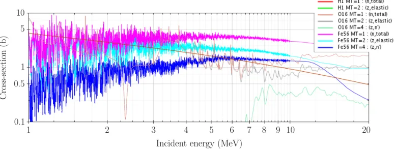
Figure I.2: Cross sections of56_Fe,16_{O and}1_{H for various reactions MT depending on the} incident neutron data

JEFF-3.3 evaluation from JANIS Books

In thermal reactors, fissions mostly result from the absorption of slow neutrons by nuclei of high atomic number. The nucleus splits into two lighter nuclei, called fission fragments and often produces an average of 2.5 neutrons with an energy of about 1 MeV or more, which will in turn interact with matter. Most of the fast neutrons which escape from the core are scattered back by the reflector and slowed down by water, which acts as a moderator, until they reach thermal equilibrium. During elastic scattering, the speed and direction of a neutron are changed due to elastic collisions with a nucleus. In water reactors, hydrogen (see Fig. I.2) is a good neutron moderator because of its mass, which is almost identical to that of a neutron. During a collision with hydrogen, the neutron thus loses a part of its kinetic energy and hence slows down.

If the energy of the incident neutron is close to the energy of an excited state of the nucleus, resonance peaks can also be observed, revealing the quantum nature of nuclear interactions. Resonances are often observed in the epithermal range, where cross sections can vary very quickly. For the major structural materials, as56_{Fe (Fig. I.2), the resonance region is extended} up to 1 MeV. Another property of the56_{Fe in ﬁssion reactors is its ability to slow down fast} neutrons by inelastic scattering.

(22)

2. BOLTZMANN NEUTRON TRANSPORT EQUATION IN ISOTROPIC BOUNDED DOMAIN

2 Boltzmann neutron transport equation in isotropic bounded

do-main

The neutron transport equation describes the distribution of neutrons in space, energy and time. There are two main forms of neutron transport equation which involves diﬀerent techniques of resolutions:

• the integro-diﬀerential form which expresses the balance between neutron loss and gain in a volume element and which is explicitly solved by the deterministic codes,

• the integral form where the transport process is viewed from the perspective of an in-dividual neutron instead of dealing with the entire neutron population described by the ﬂux.

2.1 The integro-diﬀerential equation

The integro-diﬀerential equation gives a balance statement of neutrons in a time range dt around the point (�r, E, �Ω) of the phase space and on elementary volume d�r.dE.d�Ω (Reuss,2012), where �r,E,�Ω respectively describe the space, the energy and the direction of motion (�Ω = �v_v). The angular neutron ﬂux ψ(�r, E, �Ω, t) models the neutron density per unit volume at the time t and assuming that:

 

_{On the contour area ∂V, ψ(�r, E, �Ω, t) = 0}ψ(�r, E, �Ω, t = 0) = ψ0(�r, E, �Ω) (I.1) The scalar ﬂux Φ(�r, E, t) is obtained by integration of the angular ﬂux over all directions:

Ψ(�r, E, t) = �

4πψ(�r, E, �Ω, t)d

2_Ω._� _(I.2)

Using the scalar ﬂux Ψ(�r, E, t), it is consequently possible to determine the quantity of in-terest in neutron transport analysis, i.e. the rates of neutron-induced reactions throughout the reactor core which is an observable quantity deﬁned by:

τ(�r, E, t) = N(�r, t)σ(E)Ψ(�r, E, t) = Σ(�r, E, t)Ψ(�r, E, t), (I.3) where N(�r, t) is the density of nuclei, and σ(E) and Σ(�r, E, t) are the microscopic and the macroscopic cross sections which measure the probability that a neutron has an interaction respectively per target nucleus and per centimetre path length.

For easier modelling of the interactions between neutrons and nucleus, some assumptions are considered and allow writing the transport equation.

(23)

The variation of the angular ﬂux in time 1_v∂ψ(�r,E,�Ω,t)_∂t thus results from the balance between gain and loss of neutrons:

• The term of streaming of neutrons within space and energy, and the term of the total neutron collision rate determined by the total cross section, Σt(�r, E, t)

Lψ(�r, E, �Ω, t) = �Ω.�∇ψ(�r, E, �Ω, t) + Σt(�r, E, t)ψ(�r, E, �Ω, t). (I.4) • The term of neutron scattering from the initial energy E�_{and direction Ω}� _{into energy E}

and direction Ω, Hψ(�r, E, �Ω, t) =� ∞ 0 dE �� 4πd 2_Ω_��_Σ S(�r, E� → E, �Ω� → �Ω, t)ψ(�r, E�, �Ω�,t). (I.5) In nuclear reactors, mediums can be considered as isotropic, making the scattering cross sections dependent only on the energy transfer E� _{→ E, and on the relative deviation} � Ω.�Ω�: Hψ(�r, E, �Ω, t) ≈� ∞ 0 dE �� 4πd 2_Ω_��_Σ_S_{(�r, E}�_{→ E, �Ω.�Ω}�_,_{t)ψ(�r, E}�_{, �}_Ω�_,_t) _(I.6) • The term of neutron source emitted isotropically by ﬁssion and obtained from the spec-trum χi(E, E�_{) for each ﬁssile isotope i present in the core and for ν(E}�_{) the average} number of neutrons emitted1_:

Qf iss(�r, E, t) = 1 4π � i � _∞ 0 dE

�_χ_{i(E, E}�_)(νΣ)_{f,i(�r, E}�_,_{t)φ(�r, E}�_,_t), _(I.7)

• The term of external source,

Qext(�r, E, �Ω, t). (I.8)

Often, the external source is neglected Qext=0 in PWR studies.

Finally, the Boltzmann’s operatorsH, L give the following transport equation: 1

v

∂ψ(�r, E, �Ω, t)

∂t +Lψ(�r, E, �Ω, t) = Hψ(�r, E, �Ω, t) + Qf iss(�r, E, t) (I.9) Boltzmann integro-diﬀerential transport equation

2.2 The steady state integro-diﬀerential equation

Several basic types of neutron transport problems exist, depending on the type of problem being solved. Usually, a stationary solution of the transport equation is sought and the temporal vari-ations are generally approached by a succession of steady states. Let consider for the following sections, the stationary ﬂux φ(�r, E).

(24)

2. BOLTZMANN NEUTRON TRANSPORT EQUATION IN ISOTROPIC BOUNDED DOMAIN 2.2.1 The critical equation

A fission reactor is by definition a multiplying system. It means that the time evolution of a neutron population depends on the neutron balance, i.e. the ratio between productions and losses described in the Eq. I.9. If productions and losses exactly balance, the neutron flux is constant. Most of the time, reactors operate at a constant power, i.e. with a constant number of neutrons. In such conditions, the flux is distributed on the critical mode which satisfies the steady-state neutron transport equation.

For simulating all the possible reactor states (critical, subcritical, supercritical) without hav-ing to solve a time-dependent equation, it is still possible to guarantee the balance between gain and loss of neutrons in the equation, and thus the stationarity. It consists in artiﬁcially adjusting the source term by dividing it by an eﬀective multiplication factor ke f f.

Mathematically, the ke f f corresponds to the eigenvalue of the neutron transport problem: Lψ(�r, E, �Ω) = Hψ(�r, E, �Ω) + 1

ke f fQf iss(�r, E) (I.10) Steady-state transport equation for critical calculations

In that way, three interpretations of the eﬀective multiplication factor appear:

• ke f f =1 - The reactor is critical. There is a perfect balance between production and loss of neutrons,

• ke f f <1 - The reactor is sub-critical. The removal of neutrons excesses the ﬁssion process and the chain reaction is not maintained,

• ke f f >1 - The reactor is super-critical. There is a growth of the neutron population. 2.2.2 The steady-state equation at ﬁxed sources

For the estimation of the reactor vessel ﬂux, the common approach is to perform stationary ﬁxed-source transport calculations. It consists in imposing a known neutron source Q which results from a previous critical calculation and in determining the resulting neutron distribution throughout the problem by solving the stationary Boltzmann equation.

Lψ(�r, E, �Ω) = Hψ(�r, E, �Ω) + Q(�r, E, �Ω) (I.11) Steady-state transport equation with ﬁxed sources

(25)

So, let us reconsider the integro-diﬀerential form of the steady-state neutron transport Eq.I.11. By expressing the position of a neutron as a function of its curvilinear abscissa s along its tra-jectory, and considering variations of φ around the point �r = �r0− s�Ω, we can write the following equation: −dsdψ(�r0− s�Ω, E, �Ω) + Σt(�r0− s�Ω, E)ψ(�r0− s�Ω, E, �Ω) = � � ΣS(�r0− s�Ω, E�→ E, �Ω.�Ω�)ψ(�r0− s�Ω, E�, �Ω�) + Q(�r0− s�Ω, E, �Ω) (I.12)

The curve passing through the point �r0is the straight path followed by a neutron arriving in �r0at the energy E since its last collision. Before the integration of the variations of the ﬂux along the straight line leading to the point �r, we introduce an integrating factor deﬁned as the probability that a neutron has to reach (�r, E, �Ω) without collision: e−τ(s)_{where τ(s) =}�s

0 Σt(�r0−s�Ω,� E, �Ω)ds� is the optical distance illustrated in Fig. I.3.

Figure I.3: Characteristic curve

Considering that: d ds � e−τ(s)_ψ(�r0_{− s�Ω, E, �Ω)}� = e−τ(s)�_−Σ_t_(�r0_{− s�Ω, E)�Ωψ(�r}₀_{− s�Ω, E, �Ω) +} d dsψ(�r0− s�Ω, E, �Ω) � , (I.13)

we can then write, thanks to the Eq. I.12, the following relation:

−dsd � e−τ(s)_ψ(�r0_{− s�Ω, E, �Ω)}� = e−τ(s)�� _ΣS_(�r0_{− s�Ω, E}�_{→ E, �Ω.�Ω}�_)ψ(�r0_{− s�Ω, E}�_{, �}_Ω�_{) + Q(�r0}_{− s�Ω, E, �Ω)}� (I.14)

To integrate this equation over the characteristics s from 0 to s0and consider the presence of boundaries, we assume that there is a value s0such that outside this boundary the ﬂux is null.

(26)

3. SOLVING THE NEUTRON TRANSPORT EQUATION

Finally, the steady-state integral equation is given by: ψ(�r, E, �Ω) =� s0 0 ds exp � −�₀sΣt(�r0− s�Ω,� E)ds��S (�r0− s�Ω, E, �Ω) +�₀s0ds exp�−�₀sΣt(�r0− s�Ω,� E)ds��ΣS(�r0− s�Ω, E�→ E, �Ω.�Ω�)ψ(�r0− s�Ω�,E�_{, �}_Ω�₎ (I.15) The angular ﬂux ψ(�r, E, �Ω) thus results from the two terms at the right-hand side of Eq. I.15:

• The ﬁrst is the source S (�r0− s�Ω, E, �Ω) of neutrons emitted at �r = �r0− s�Ω and at the energy E in the direction �Ω.

• The second is the term of neutron scattering ΣS(�r0− s�Ω, E� _{→ E, �Ω.�Ω}�_{) from the} initial energy E�_{and direction Ω}�_{into energy E and direction Ω.}

Integral steady-state transport equation with ﬁxed sources

3 Solving the neutron transport equation

As explained previously, there are two general approaches for solving the transport equation and modelling neutron evolution within a reactor:

• the deterministic method based on the integro-diﬀerential equation I.9 which can be sim-pliﬁed with suitable approximations, for example, with the discretisation of the phase space and on the numerical methods involving the spatial and energetic processing of the neutron propagation,

• the stochastic method which simulates the motions of many neutrons to model how they interact with matter, and statistically solves the exact complete integral form of the trans-port equation.

The choice of the method depends on the criteria of speed and accuracy required for calcu-lations. The random sample necessary to accurately describe the diﬀerent possible directions of neutrons makes the use of stochastic methods expensive. However, with improved computing performance, they are being increasingly used as reference calculations because they provide a more accurate description of the reactor physics. On the other hand, deterministic methods are often preferred for quick ﬁrst-hand calculations. The following sections therefore introduce both solving approaches.

(27)

3.1.1 Energy discretisation by multigroup formalism

Most deterministic methods use a multigroup approach based on the energy discretisation. The energy is in fact discretised in diﬀerent intervals called groups that form a multigroup mesh. The number of energy groups depends on the desired precision for simulations and on the energy domain studied. In that sense, it is possible to convert each term of the Eq. I.11 in a multigroup form:

�

Ω.�∇ψg(�r, �Ω) + Σg_t(�r)ψg(�r, �Ω) = Qg(�r, �Ω). (I.16) Multigroup and diﬀerential form of the steady-state transport equation

In practice, the multigroup discretisation may be performed in many instances of a compu-tational scheme. The ﬁrst energy condensation occurs when the NJOY Nuclear Data Processing System (MacFarlane,2017) convert pointwise data into multigroup form, as discussed later in Section 4.3. The next energy condensation can then arise in lattice code to energetically con-dense and spatially homogenise the cross section data into the structure needed for the reactor core calculation.

Specifically, multigroup cross sections are defined following conservation of the multigroup reaction rate σg_(�r)φg_{(�r), that is, equalising the integral value of the pointwise reaction rate} σ(E)φ(�r, E) on the group g. For each group of the energy mesh, the multigroup cross section is thus defined by:

σg(�r) = �

gσ(�r, E)φ(�r, E)dE

φg(�r) , (I.17)

where φg_{(�r) =} �

gφ(�r, E)dE is the multigroup ﬂux solution of the Boltzmann multigroup equation.

This formalism, however, raises several practical diﬃculties (Coste-Delcaux,2006): • the pointwise ﬂux φ(�r, E) is unknown,

• the multigroup ﬂux φg_{(�r) is solution of the Boltzmann multigroup equation for which the} multigroup cross sections are the input parameter of deterministic codes,

• the multigroup cross sections are intrinsic to the geometry of the problem to solve. To create cross sections which are independent of the geometry, an alternative method con-sists in replacing the ﬂux in the equation I.17 by a weight function w(E) which is representative of the spectrum and independent of position. The multigroup cross sections are thus said to be at inﬁnite dilution: σg_≈ � gσ(E)w(E)dE � gw(E)dE . (I.18)

The approximation is acceptable for non-resonant nuclei for which the cross section is rel-atively smooth but it is not sufficiently accurate for the resonant nuclei when the energy mesh is too broad. In fact, the existence of resonances leads to a depreciating flux. This phenomenon is called energy self-shielding, and it is the more influential the greater the concentration of resonant nuclei is. To capture efficiently the self-shielding effect, the first possibility is to refine energy mesh taking an exact account of the variations of cross sections and flux. The problem is that the calculation time strongly depends on the energy group number. Another possibility is to employ a self-shielding method as the Livolant-Jeanpierre and the subgroup methods (Livolant and Jeanpierre,1974;Coste-Delcaux,1996).

(28)

3. SOLVING THE NEUTRON TRANSPORT EQUATION 3.1.2 Approximation of angular dependence by the SN method of discrete ordinates To derive the angular dependence, one of the best-established methods is the collocation method of discrete ordinates (SN). The method consists in choosing M = N(N + 2) isolated directions (ordinates) ω = {�Ωm; m = 1..M} as:

ψ(�r, �Ω) ≈  

ψ(�r, �Ωm) if �Ω = �Ωm_{0 and �Ω � ω}and �Ωm∈ ω (I.19)

The steady-state transport equation I.11 with ﬁxed sources can thus be written for one group g and one direction m as:

Lgmψg(�r, �Ωm) =Hgmψg(�r, �Ωm) + Qg(�r, �Ωm), (I.20) with Lgmψg(�r, �Ωm) = �Ωm.�∇ψg(�r, �Ωm) + Σgt(�r)ψg(�r, �Ωm), (I.21) Hgmψg(�r, �Ωm) = � 4Πd�Ω �_{Σs(�r, g}� _{→ g, �Ω}_m.�_Ω�_)ψg_{(�r, �Ωm),} _(I.22) and evaluating the angular integral by the Wick quadrature formula (Lee,1961) with M weights ωm: 1 4Π � 4Πd�Ω f (�Ω) = M � m=1 � Ωmf (�Ωm), (I.23)

SNangular discretisation of the steady-state transport equation with ﬁxed sources

Usually the M directions and weights are ﬁxed by a Gauss quadrature formula. The resulting system of M equations is thus solved and the ψg_{(�r, �Ωm)s are the unknowns of the system.} 3.1.3 Spatial discretionary by discontinuous ﬁnite element

The last approximation used for solving partial differential equations is the spatial discretisation. In particular, the method of discontinuous finite element can be associated with an SNapproach for a mesh-by-mesh resolution that does not require the resolution of the overall system of un-knowns. It consists in expressing the flux on each mesh C as a basis function (polynomial) w in the projection space and without imposing the continuity of flux at interfaces among neighbour mesh.

(29)

3.2 Monte Carlo method

The Monte Carlo method was introduced by John Von Neumann and Stanley Ulam. This method allows ﬁnding a statistical solution to the integral equation I.15 where the transport process is viewed from the perspective of an individual neutron instead of dealing with the entire neutron population when solving the integro-diﬀerential form.

3.2.1 Stochastic neutron propagation by Markovian process

Let us now reconsider the integral equation introduced in the previous section 2.3. By using the following identity: � ∞ 0 f (�r0− s�Ω)ds = � f (�r) � δ(�Ω − �r0− �r |�r0− �r|) � _d�r |�r0− �r|2, (I.25) the line integral equation can be transformed into a volume integral equation (Vassiliev,

2017).

To simplify the notations, one commonly deﬁnes the two following kernels (Nowak,2018): • the transition kernel, i.e. the probability density for a particle at �r to reach the distance

s = |�r0− �r| without collision and to be subject at a collision at �r0, T(�r → �r0,E, �Ω) = Σt(�r0− s�Ω, E)e−τ(s) � δ_{(�Ω −} �r0− �r |�r0− �r|) 1 |�r0− �r|2 � , (I.26) • the collision kernel, i.e. the probability for a particle entering a collision at (�r0,E�, �Ω�) to

be scattered in energy E and direction �Ω,

C(�r0,E� _{→ E, �Ω}� _{→ �Ω) =} ΣS(�r0− s�Ω, E�→ E, �Ω.�Ω�) Σt(�r0− s�Ω, E)

. (I.27)

The two kernels allow introducing the collision density deﬁned as τ(P) = Σt(P)φ(P), the rate at which particles undergo a collision at P:

τ(P) = S1(P) + �

τ(P��_)dP�_P��_, _(I.28)

where S1is the source of the ﬁrst collision.

The collision density can also be written as a Neumann series expansion: τ(P) =�∞

n

τn(P). (I.29)

Each term of this series can be obtained by recurrence of the previous one following the formulation:

τn(P) =� ... �

S (P0)T(P0 → P1)K(P1→ P2)...K(Pn−1→ P)dP0P1...dPn−1, (I.30) such as K(P� _{→ P) = T(P}� _{→ P)C(P}�� _{→ P).}

Eq. I.30 shows that the state of the neutron at the step n is determined by the state of the neutron at the previous step n − 1. The random process of the neutron propagation thus follows a Markovian process. The resolution of the integral neutron transport equation can thus be achieved by simulating a chain of events which constitutes the history of each neutron source.

(30)

4. NUCLEAR DATA EVALUATION 3.2.2 Analogue simulation

We can now understand how the Monte Carlo approach simulates the stochastic nature of neu-tron transport through matter, i.e. by tracing the random walk of an individual neuneu-tron in matter and considering the various interactions that may determine its history.

Let us imagine the behaviour of a single neutron from its source to a tally (a detector). In a nuclear reactor, the fission is the main source of neutrons. The fission source can be described by its distribution in space (directly linked to the power of assemblies in the reactor), its distribution in energy (defined by a spectrum) and its distribution in direction (often considered as isotropic). These distributions can be characterised by a cumulative probability distribution function which allows randomly defining a location and an energy for any considered neutron. The random walk and the state of the neutron then depend on the geometry of the crossed domain and on the physical properties of the matter. The distance to the next collision and the type of the next interaction are thus sampled following the total cross sections. If the reaction type is absorption, the neutron history is terminated, the energy and location of the absorbed neutron are recorded, and another history is started. If a scattering event is sampled, the direction and the energy of the considered neutron are changed and a new sampling occurs to determine the distance to the next collision. If the sampled interaction is fission, a number of neutrons are produced, and so on. Finally, to determine the flux at the specific position of the detector, the Monte Carlo approach simulates many neutron random walks and counts the neutrons reaching the detector.

The procedure just described is usually called the analogue scheme meaning that the parti-cles are transported in a way corresponding to the physical interactions with matter. The ana-logue simulations use in fact the fundamental conservation laws (energy momentum, angular momentum, etc.) which describe the physical phenomena encountered by the neutron during its way.

3.2.3 Non-analogue simulation

One of the issues with the Monte Carlo approach is the slow convergence of its calculations due to the limited number of simulated trajectories. To limit the statistical error on results, Monte Carlo codes must simulate a large number of particles, making simulations too time-consuming. Moreover, the analogue simulation remains ineﬃcient to simulate the neutron population in nuclear reactors. in consequence it becomes favourable to use biasing techniques or variance reduction techniques for emphasising neutrons that are most likely to contribute to the tally. This type of simulation is usually known as the non-analogue scheme. It consists in associating weight with neutrons and adjusting the neutron weight at each event in its history (Marguet,

2011). For example, the weight decreases for neutron-absorbing media. A threshold s is then used conditionally to ignore any neutron with a contribution that is too low, and for which continuing the path would be useless. Other approaches can ignore the neutrons that are in an uninteresting part of the phase space, such as the Russian roulette method. Depending on the physical systems simulated, many other diﬀerent methods are used for non-analogue schemes to accelerate Monte Carlo simulations (Nowak,2018).

(31)

following sections. They are based on the tools and codes, the purpose of which is aiming to provide a better modelling of the physical data, to estimate the associated uncertainties and to reduce the calculation bias.

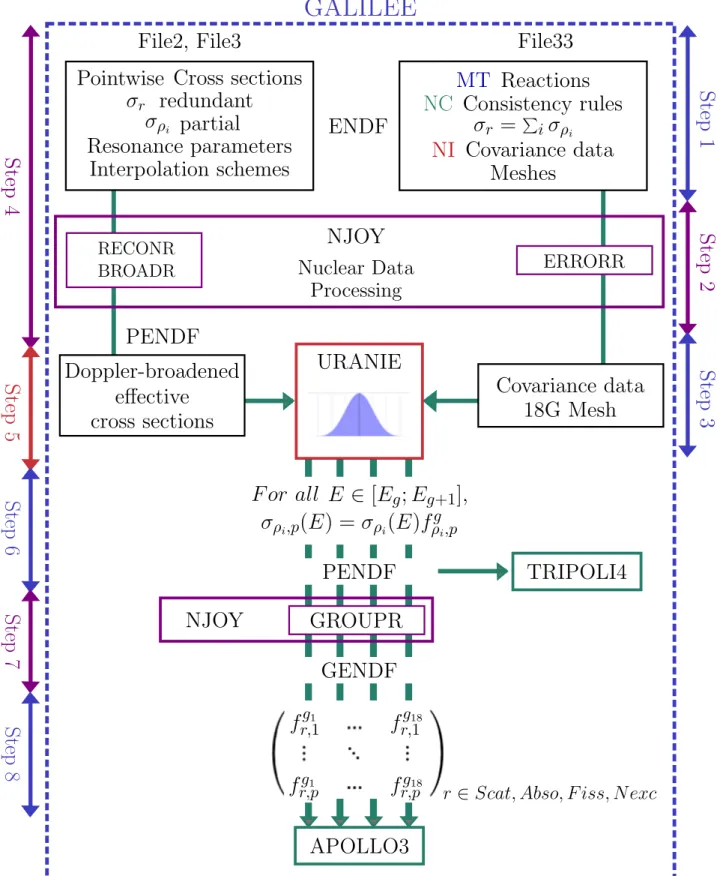
Figure I.4: Multigroup data generation for deterministic codes.

4.1 From experiments to libraries

The nuclear data are given using the standardised format ENDF in international libraries as for example ENDF/B-VII (the American Library) (McLane,2005), JEFF-3 (the European library) (JEFF-3.1,2013), JENDL-4 (the Japan Library) (JENDL-4.0,2011).

Libraries contain the fundamental physical parameters needed for modelling nuclear inter-actions for several incident particles and for a large set of materials and isotopes. Because of the complexity of nuclear interactions and the incapacity of theory to describe them accurately, pa-rameters are often deﬁned by the iterative evaluation process combining validated physical mod-els and data assimilation experiments. It consists in involving Bayesian inferences (Kessedjian,

2015) to adjust the theoretical parameters of models by maximum likelihood and by reducing uncertainties. Two types of experiments are used for this evaluation. Differential experiments allow measuring microscopic quantities as functions of the energy of the incoming particle, such as cross sections, fission yields and angular distributions. Integral experiments measure macro-scopic quantities as cross sections integrated on neutron flux and can then be used for validating and adjusting nuclear data libraries. The resulting evaluated nuclear data corresponds to the best estimates of the quantities of interest, i.e. the mean values as defined in the next section 1 of Chapter II.

4.2 Sources of uncertainties in nuclear data evaluations

In practice, nuclear data cannot be accurately estimated because in the evaluation process, there exist a succession of sources of uncertainties which can be divided in two types:

(32)

4. NUCLEAR DATA EVALUATION • Aleatory uncertainty due to the random nature of the system or to the statistical eﬀects of detection in microscopic experiments. These can be handled by repeating independent measurements under the same conditions. Following the central limit theorem, one can then determine the best estimates and associated variances,

• Epistemic uncertainty which produces systematic errors, for example, due to the methods of measurements and reconstructions (normalisation, background subtraction, calibration, etc.) or due to the measurement resolution which can be identiﬁed by diversifying the methods and instruments.

The ﬁnal uncertainty of a quantity of interest results thus from the propagation of these uncertainties on the iterative evaluation process. As explained in the previous Section 4.1, the uncertainty quantiﬁcation is carried out during the data evaluation process, and generally, fol-lowing a Bayesian approach that provides a better assessment of the uncertainty than the fre-quentist approach (King et al.,2019;Kessedjian,2015).

In data libraries, the characterisation of uncertainties is given by covariance matrices. The latter encloses two types of information: the accuracy of each evaluated data, encoded in the variances, and the correlations among data, which reveal their consistency and the analysis choices during their evaluation process. In fact, the evaluated data tend to be correlated for sev-eral reasons. Some parameters can for example be involved in evaluation of different data. Some adjustment processes can also create correlations among data (as normalisation, marginalisation, consistent adjustment, ...) (Privas,2015). The covariance data defined in a library is thus evalu-ated following the methodology adopted to obtain the central values of the nuclear data defined in the same library. This is why they are attached to the data of their own library.

In the ENDF format (McLane,2005), the nuclear data which describe the neutron interac-tions are given in the Files from 1 to 5 and the corresponding covariance data are provided in sections MF-31-32-33-34-35 as presented in Tab. 2. Specifically, the MF32-file and the MF33-file give the covariances, respectively, on the resonances parameters (MF2) and on the pointwise cross sections (MF3).

Data Files Corresponding Covariances

The average number of neutrons per ﬁssion MF1-MT452 MF31

Resonance parameters MF2 MF32

Neutrons cross sections MF3 MF33

Angular distribution of secondary particles MF4 MF34

Energy distribution of secondary particles MF5 MF35

Table I.1: Transport data for the description of neutron interactions

4.3 NJOY treatments for simulation codes

As explained previously, the interaction between a neutron and a nucleus depends on the energy of the incident particle and on the temperature of the target. The energy dependence can be described by a pointwise or a multigroup formalism.

(33)

4.3.1 Generation of point-cross sections in PENDF Files

• RECONR - The ﬁrst step of treatment is to rebuild the pointwise values as a function of the neutron incident energy in the laboratory frame of reference for a target nuclei in the ground state (T = 0K) from ENDF resonance parameters and interpolation schemes. Interpolation schemes consist in describing nuclear data by a set of points associated with an interpolation law (linear or cubic) which allows rebuilding the data for any parameter value (incident energy or temperature).

• BROADR- The pointwise values are then broadened considering the Doppler eﬀect by convolution of the "0K" values with the velocity distribution of the target nuclei. At this step, the cross sections can be used by the Monte Carlo codes and are deﬁned following a PENDF-format.

• UNRESR, HEATR, THERMR- Some modules can also compute cross sections for spe-ciﬁc energy ranges or applications. The module UNRESR computes, for example, eﬀec-tive self-shielded pointwise cross sections in the unresolved energy range. HEATR gen-erates pointwise heat production cross sections and radiation damage production cross sections. THERMR produces cross sections and energy-to-energy matrices for free or bound scatterers in the thermal energy range.

4.3.2 Generation of multigroup cross sections in GENDF Files

• GROUPR- For the deterministic codes, the cross sections rather should be converted to multigroup formalism as deﬁned by Eq. I.18. It generates various types of multigroup data: self-shielded multigroup cross sections, group-to-group scattering matrices, photon production matrices, and charged-particle multigroup cross sections from pointwise input. At the end of the GROUPR process, the multigroup data are provided in a GENDF-format. a Multigroup cross sections The cross sections are given by weighting the pointwise cross sections σ(E) on the multigroup spectrum w(E) and following the concept of gen-eralised group (with a feed function F(E) = 1):

σg= � gσ(E)w(E)dE � gw(E)dE . (I.31)

b Two-body multigroup scattering The two-body multigroup scattering cross sec-tions are calculated according to the Bondarenko ﬂux weighting model (MacFarlane,

2017) and the concept of a generalised group:

σg_l�→g= �

g�F

g

l(E�)σ(E�)w(E�)dE� �

g�w(E�)dE�

, (I.32)

– σ(E�_{): the pointwise microscopic cross section at E}�_, – w(E�_{): the weight function at E}�_,

– Fg_l: the l-th Legendre component of the normalised probability of scattering into arrival energy group g from initial energy E�_.

(34)

4. NUCLEAR DATA EVALUATION In the case of elastic and inelastic neutron scattering, the output energy E is completely determined by the E� _{incident energy and the center-of-mass cosine of the scatter angle} ω:

ω = E(1 + A)

2_{− E}2_{(1 + R}2₎

2RE� , (I.33)

The relation between the center-of-mass and the laboratory cosines of the scatter angle are related by:

µ = _√ 1 + Rω

1 + R2₊_2Rω, (I.34)

where A is the ratio between the target mass to neutron mass of the neutron and R is a function of the energy level of the excited nucleus (Q = 0 and R = A for elastic scattering). The feed for two-body scattering is computed using a Gaussian integration scheme with the f (E� _{→ E, ω) = f (E}�_{, ω}_{) probability of scattering from E}�_{to E through a} center-of-mass cosine ω:

Fg_l(E�_{) =}� ω2(E

�₎

ω1(E�)

f (E�_{, ω)Pl[µ(ω)]dω.} _(I.35)

ω1(E�) and ω2(E�) are evaluated for E equal to respectively the upper and lower bounds of g�_{. Pl}_{is deﬁned from the Legendre polynomials.}

The scattering probability is given by a Legendre polynomial series: f (E�_{, ω}_{) =}�L

k=1 2k − 1

2 ak(E�)Pk(ω), (I.36)

where the Legendre coeﬃcients ak(E�_{) are retrieved from the ENDF File 4. Equations} I.32 and I.36 introduce ﬁnally the angular distribution and the correlation between the energy of the incident neutron and the emission angle after the scattering process. 4.3.3 Reconstruction of multigroup covariances with the module ERRORR

• ERRORR

-The module ERRORR ofMacFarlane(2017) converts energy dependent covariance infor-mation in ENDF format into multigroup form by combining the covariance inforinfor-mation from the File 33 with the data of the File 3 (defined Section 4.2, see Table4.2) . This calcu-lation is based on the creation of an input script which describes the input instructions and specifications needed to generate the desired covariance matrix. In an ERRORR input, the instructions are presented in a card format (see Manual NJOY,MacFarlane(2017)). Each card is parametrised by a list of options which define the different steps of the ERRORR process, and by a succession of "tape" which refers to intermediate input or output files

(35)

(36)

Chapter II

Statistics Background

Uncertainty analysis are increasingly being used in nuclear calculation (neutron dosimetry, re-actor design, criticality assessments, etc.) to deduce the accuracy of safety parameters (fast fluence, reactivity coefficients, criticality, etc.) and to establish safety margins. Generally, the calculation of quantities of interest results from the implementation of successive physical mod-els, which depend on uncertain inputs and on assumptions relative to methods involved for the calculation itself. The inaccurate evaluation of quantities thus results from the combination be-tween modelling errors, numerical errors and the propagation of input uncertainties through the simulation tools. Under these circumstances, sensitivity analysis evaluate the impact of input uncertainties in terms of their relative contributions to uncertainty in the output. They help to prioritise efforts for uncertainty reduction, improving the quality of the data.

The intent of this chapter is thus to present the background needed to carry out uncertainty analysis and sensitivity analysis in the context of nuclear models.

1 Basic concepts in modelling uncertainty

1.1 First and Second Central moment

Let us consider a real parameter y which results mathematically from the interactions of real input parameters, described by y = f (x) and as illustrated by Fig. II.1. In that context, the aim of uncertainty analysis is to determine the output uncertainty of y considering the uncertainties of input parameters x1, ...,xn.

(37)

CHAPTER II. STATISTICS BACKGROUND

P, the probability measure. The multivariate probability distribution of the random vector X is characterised by the Cumulative Distribution Function (CDF), such as:

FX(x1,x2, ...,xn) = P(X1≤ x1and X2≤ x2, ..., and Xn≤ xn), (II.1) and which obeys the following conditions:

FXis monotone increasing, F_X(x1 =−∞, x2=−∞, ..., xn =−∞) = 0 FX(x1 = +∞, x2= +∞, ..., xn = +∞) = 1

(II.2) The joint Probability Density Function (PDF), can then be computed as a partial derivative of Eq. II.1: p_X(x) = ∂nFX(x) ∂x1∂x2...∂xn �� _x, (II.3) wherex = x1,x2, ...,xn.

As expressed by Eq. II.2, FX provides a complete representation of the set of n random variables, and consequently, p_Xis normalised:

� x1 ... � xn pX(x)dx1dx2...dxn=1. (II.4)

For i = 1, .., n, we can also deﬁne the marginal density function associated with the variable Xi alone, by integrating pXover all values of the other n − 1 variables:

pXi(xi) =

�

pX(x1,x2, ...,xn)dx1...dxi−1dxi+1...dxn= �

px(x−i,xi)dx−i. (II.5) In this way, the distribution of the random variable Xiadmits a probability density function, and the expectation of Xican therefore be calculated as the ﬁrst central moment:

E[Xi] = �

xi

xipxi(xi)dxi. (II.6)

Expectation

In the same way, we can assess the joint probability density function of two random variables X1, X2:

pX1,X2(x1,x2) =

∂2F_X(x1,x2)

∂x1∂x2 , (II.7)

with FX(x1,x2) = P (X1 ≤ x1and X2≤ x2), is straightforwardly derived by integrating pX over all variables other than X1and X2.

In this respect, one important quantity is the covariance between X1and X2which measures the joint variability of the two variables, expressed as the second central moment:

cov(X1,X2) = �

x1

� x2

(x1− E[X1])(x2− E[X2])pX1,X2(x1,x2)dx1dx2. (II.8)

(38)

2. LINEAR MODELS Finally, we consider the random variable Y which describes the probability distribution of y = f (x), expressed by Y = f (X). It is straightforward to derive its expectation value:

E[Y] = E[ f (X)] =�

S (x) f (x)px(x)dx. (II.9)

The uncertainty of Y is deﬁned as the standard deviation σY which is the square root of the variance var ( f (X)), another quantity expressed by a second central moment:

Var[Y] = σ2Y =E[( f (X) − E[ f (X)])2]. (II.10) Uncertainty

1.2 Maximum entropy probability distribution

In practice, the full joint probability density function p_X(x) is not all the time known. To circumvent this lack of information, one key concept is the information entropy introduced by Shannon (Shannon,1948). The corresponding formula for a continuous random variable X with a probability density function pX(x) is given by:

h �p� = �

xpX(x)ln(pX(x))dx. (II.11)

When some information is provided (for example, the ﬁrst and second central moments) but not enough to describe the full probability distribution of a variable, the principle of maximum entropy, ﬁrst expounded by Jaynes (Jaynes,1957), states that the probability distribution which best represents the current state of knowledge is the one with largest entropy h �p�. In partic-ular, when the mean µ and the variance σ2_{is selected as descriptors of the data, the Gaussian} distribution (N(µ, σ2_{)) is the best distribution to represent the information entropy. For some} other practical cases, when the minimum and maximum values a and b are known, the uniform distribution (U(a, b)) is the distribution which maximises the entropy.

2 Linear models

When it comes to studying the variation of a model output, linear models can be very profitable because they can readily simplify the setting up of regression, uncertainty quantification and sensitivity analysis. The main question is whether a linear regression is sufficient to model the behaviour of a random variable Y in the range of uncertainties of inputs.

To illustrate this, one can consider an experimental design with p observations of n input variables and of the corresponding output response y of a model. The estimation of a linear regression consists in assessing, from the observed measurements, a vector of unknown

(39)

param-CHAPTER II. STATISTICS BACKGROUND

It is assumed that each observation ykof Y satisﬁes:

yk = β0+xkβ + �k, (II.13)

wherexk∈ Rnis the k-th observations of the n variables (x1, ...,xn), and denoted as:

xk =�x(k,1) · · · x(k,n)�, (II.14)

�k is a zero-mean Gaussian noise, as for all k the random variables �k are independent and identically distributed (�k � N(0, σ2). We can thus assume the fact that:

E(Y|x1, ...,xn) = β0+xkβand Var(Y) = σ2. (II.15) The matrix format of Eq. II.13 gives:

Y = Xβ + �, (II.16) where, X =     1 x(1,1) · · · x(1,n) .. . ... ... ... 1 x(p,1) · · · x(p,n)    ,X ∈ R

p×n_{is the design matrix,} _(II.17)

Y =�y1 · · · yp�t,Y ∈ Rpis the response vector, (II.18) β =�β1 _{· · · β}n�t, β∈ Rnis the coeﬃcient vector, (II.19) � =��1 _{· · · �}p�t,� ∈ Rpis the error vector. (II.20)

In the case where the number of samples p is greater than the number of input variables n, and the Xt_{X is a positive-deﬁnite matrix, the optimal coeﬃcient vector β of a linear} regression problem is given by the Ordinary Least Squares which states that assuming the Gaussian distribution of the error �, the maximum likelihood estimator is:

ˆβ = arg min

β∈ Rn ||Y − Xβ||

2

2. (II.21)

The minimisation II.21 gives then:

ˆβ = (Xt_X)−1_Xt_Y, _(II.22)

in the case where matrix X is of full rank.

Ordinary Least Squares

Since all outcomes yk are equiprobable, Eq. II.6 gives the mean of the observed data ¯y as: ¯y = 1 p p � k=1 yk. (II.23)

Empirically, the variability of the data set can then be measured using three following classic formulas SST, SSRes,SSReg(related by SST = SSReg+SSRes):

(40)

3. UNCERTAINTY QUANTIFICATION • The total sum of squares (total variance),

SST = p � k=1

(yk− ¯y)2, (II.24)

• The explained sum of squares,

SSReg= p � k=1

(ˆyk− ¯y)2, (II.25)

• The residual sum of squares,

SSRes= p � k=1 (yk− ˆyk)2 ₌� k �_k2, (II.26)

where ˆyk = ˆy(xk) is the prediction resulting from the linear model.

Thereafter, to measure the quality of the linear regression, the following coeﬃcients can be calculated: R2₌_{1 −} �p k=1(yk− ˆyk)2 �p k=1(yk− ¯y)2 R2 ad j=1 − |1 − R2| �� _{p − (1 + n)}p − 1 �� Q2=1 − �p k=1(yk− ˆyk,−k)2 �p k=1(yk− ¯y)2

The coeﬃcient of determination The adjusted coeﬃcient The LOO-cross-validated R2

Table II.1:Linearity veriﬁcation

R2_{is thus expressed as the ratio of the explained variance to the total variance. When R}2_is close to 1, we can assume that the linear regression is validated. Similarly, the R2

ad jis deﬁned but it penalizes in addition the statistic if the sample size is not very great compared to the number of variables.

Moreover, Q2 _{is defined as the value of R}2_{, using the sampling data set, but where each} predicted value ˆyk,−k is given from Leave-One-Out cross validation, i.e. with a linear model ˆy(x,−k)estimated from the set of p − 1 points {1, . . . , k − 1, k + 1, . . . , p}. The numerator of Q2_is therefore defined as the Predictive Residual Error Sum of Squares defined byAllen(1974).

3 Uncertainty quantiﬁcation

There are two main methods to conduct an uncertainty analysis: the method of moments based on truncated Taylor series expansion and the Monte Carlo method. This section presents the background which will be necessary in this thesis to determine which of the methods are ade-quate to evaluate the uncertainty and to strengthen its evaluation.