HAL Id: cea-01823372
https://hal-cea.archives-ouvertes.fr/cea-01823372
Submitted on 16 Jul 2019
HAL is a multi-disciplinary open access
archive for the deposit and dissemination of
sci-entific research documents, whether they are
pub-lished or not. The documents may come from
teaching and research institutions in France or
abroad, or from public or private research centers.
L’archive ouverte pluridisciplinaire HAL, est
destinée au dépôt et à la diffusion de documents
scientifiques de niveau recherche, publiés ou non,
émanant des établissements d’enseignement et de
recherche français ou étrangers, des laboratoires
publics ou privés.
R. Coulon, J. Dumazert
To cite this version:
R. Coulon, J. Dumazert. Nuclear signal simulation applied to gas ionizing chambers. 2015 4th
Interna-tional Conference on Advancements in Nuclear Instrumentation Measurement Methods and their
Ap-plications (ANIMMA), Apr 2015, Lisbon, Portugal. pp.7465520, �10.1109/ANIMMA.2015.7465520�.
�cea-01823372�
Abstract— Particle transport codes used in detector simulation
allow the calculation of the energy deposited by charged particles produced following an interaction. The pulses temporal shaping is more and more used in nuclear measurement into pulse shape analysis techniques. A model is proposed in this paper to simulate the pulse temporal shaping and the associated noise level thanks to the output track file PTRAC provides by Monte-Carlo particle transport codes. The model has been dedicated to ion chambers and more especially for High Pressure Xenon chambers HPXe where the pulse shape analysis can resolve some issues regarding with this technology as the ballistic deficit phenomenon. The model is fully described and an example is presented as a validation of such full detector simulation.
Index Terms— Nuclear, Instrumentation, Measurement,
Simulation, Monte-Carlo, Ion Chamber, Xenon, Pulse Shape Analysis.
I. INTRODUCTION
UCLEAR instruments have always to be upgraded in order to address new industrial and societal issues as in research experiment, fuel cycle, electronuclear production, dismantling, environmental, medical and security. Particle transport codes are able to simulate the detector response in term of energy deposition. On another hand, the front-end electronic of such detectors could be designed using electronic simulation tools. In an ideal world, the design of nuclear detector requires to take into account both physics and electronics considerations. However, the results of physical simulations given by Monte-Carlo transport codes cannot directly be used as an input for electronics simulations. Indeed, the pulse signal and its associated noises are shaped by charge productions and migration process and by the coupling to the electronic conversion device. Therefore, a model allowing the pulse temporal shape and its associated noises to be simulated represents an interesting opportunity for future developments in the field of nuclear instrumentations.
Some previews works should be quoted. A pulse shape model has been developed by some laboratories for segmented germanium in order to optimize individual interaction locations using pulse shape analysis [1-3]. Some models have also been developed to simulate the pulse shape of gas detectors as in the case of fission chambers [4] or scintillation
Authors are with the French Alternative Energies and Atomic Energy Commission (CEA) F-91191 Gif-sur-Yvette, France.
(e-mail: [email protected], [email protected])
in xenon detectors [5]. The model developed in our paper addresses the simulation of ion chambers and more particularly High Pressure Xenon chambers (HPXe).
II. METHODS
The current produced by the detector and its front-end electronics can be modeled following the subsequent steps:
The charge carrier production induced by the interaction between γ-radiations and the noble gas;
A current induced at the anode of the detector by the charge carrier motion into the electric field;
A thermal leakage current and some Gaussian noises added by the components of the charge sensitive preamplifier.
The model is detailed bellow following these three parts.
A. Interaction of X and γ rays with matter
Following the interaction of an X-ray or a γ-ray into the gas, primary recoil electrons are produced by photoelectric effect, Compton scattering or pair production. Interaction data are calculated using a particle transportation program based on a Monte-Carlo method to solve the Boltzmann transport equations. The MCNPX2.7 code from LANL has been used in this study [6].
A primary recoil electron from interaction is generated into the gas medium. The path of this electron is calculated by the MCNPX program until the cut-off energy of 1 keV. The electron loses its energy intermittently due to collisions and continuously due to ionization. Bremsstrahlung radiations can also take place, escaping out of the sensor or creating a secondary recoil electron elsewhere inside the gas. Fig. 1 presents the distribution of the number of collisions calculated over 500 paths of primary electrons with a kinetic energy equal to 662 keV into the xenon gas. The number of collisions is distributed between 40 and 120 collisions with an expected collision number equal to 80. A density of 0.55 g.cm-3 and a concentration of 0.2 % of H2 is considered in this study as optimal gas mixture as reported in the literature [7-8].
Nuclear Signal Simulation Applied To Gas
Ionizing Chambers
Romain Coulon and Jonathan Dumazert
CEA, LIST, Laboratoire Capteurs et Architectures Electroniques, F-91191 Gif-sur-Yvette, France.
Fig. 1. Distribution of the number of collisions above the energy level of 1 keV calculated over 500 primary electrons with a kinetic energy of 662 keV into the pressurized xenon.
At each collision, a δ-electron is put in motion by recoil, itself slowing down by ε collisions, ionizations and excitations. The energy threshold for δ collision lies between 100 eV and 1 keV. δ-electrons have a mean energy around keV and lose their energy marginally by ε collisions and mostly by ionizations and excitations. As an illustration, the energy distribution of δ-electrons for 662 keV primary electrons in pressurized xenon is presented on the Fig. 2.
Fig. 2. Distribution of the kinetic energy of δ electrons into pressurized xenon for a 662 keV primary electron (defined from 1 keV)
The MCNP/PTRAC file containing the details of interaction data associated with primary and secondary electrons is written as an output of the calculation. A post-processing of this file is carried out to model the charge carrier production and migration.
B. Charge carrier production
The processing of a path history contained into the PTRAC allows the extraction of following data, where 𝑛𝛿 is the number of collisions along the primary recoil electron path:
𝑋1𝛿= (𝑥1𝛿, 𝑦1𝛿, 𝑧1𝛿) are coordinates of δ and ε collisions
𝑋2𝛿= (𝑥2𝛿, 𝑦2𝛿, 𝑧2𝛿) are coordinates of the end of the δ and ε electron paths.
The kinetic energy of the primary electron noted 𝐸0
The kinetic energy of δ and ε electrons noted 𝐸2𝛿
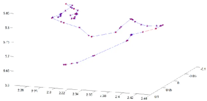
electron into pressurized xenon gas. Red stars represent collision locations and blue lines the path of the primary electron.
Fig. 3. Path of a 662 keV primary electron in pressurized xenon (unit length in cm)
At the end of the electron slowing down process, the energy density of electrons is dispatched between the paths of δ-electrons and the path of the primary electron. The dissipated energy by ionization and excitation, 𝐸1𝛿, between every collision is calculated by Eq. 2, where 𝑑1𝛿 is the distance between two successive collisions (see Eq. 1).
∀𝛿 ∈ [1; 𝑛𝛿], 𝑑1𝛿 = ( 𝑥1𝛿+1− 𝑥1𝛿) 2 + ( 𝑦1𝛿+1− 𝑦1𝛿) 2 + (𝑧1𝛿+1− 𝑧1𝛿) 2 (1) 𝐸1𝛿 = (𝐸0− ∑𝑛𝛿=1𝛿 𝐸2𝛿). 𝑑1𝛿 ∑𝑛𝛿=1𝛿−1 𝑑1𝛿 (2) The cooling time of the primary electron is in the order of the picosecond and the ionization occurs in a nanometer range around the track. The energy deposition is therefore considered as punctual in comparison with the duration of charge drifting (in the range of µs) studied below. The density of energy is therefore modeled in a linear form following spatial coordinates. A schematic of the 2-D broken line model for recoil electrons is shown in Fig 4. The first dimension 𝑗 = 1 describes the path along the primary electron with energy 𝐸1𝛿 uniformly distributed between 𝑋1𝛿 and 𝑋1𝛿+1 , the second dimension 𝑗 = 2 describes the path along 𝛿 electrons with energies 𝐸2𝛿 uniformly distributed between 𝑋1𝛿 et 𝑋2𝛿. A schematic of the 2-D broken line model for recoil electrons is shown in Fig 4.
Fig. 4. Schematic of the 2-D broken-line model.
Knowing the energy threshold allowing the product of an electron-ion pair 𝑊𝑖, expectations associated to the number of charge carrier pair 𝑁𝑗𝛿 created along the primary electron path can be calculated according to Eq. 3:
∀𝛿 ∈ [1; 𝑛𝛿], ∀𝑗 = {1; 2}, 𝑁𝑗𝛿= ‖
𝐸𝑗𝛿
𝑊𝑖‖ (3) The quantification of the number of charges is taken into account using a corrected Poisson sampling described by a Normal distribution 𝒩, centered around the expected number of charge N and with an associated variance FN where F is the Fano factor. In our model, random variables 𝑛1𝛿 and 𝑛2𝛿 correspond to the number of charges produced respectively between 𝛿 collisions and along the path of 𝛿 electrons. They are randomly drawn from a Normal distribution 𝒩 with expetations 𝑁1𝛿 and 𝑁2𝛿 and variances 𝐹𝑁1𝛿 and 𝐹𝑁2𝛿 as described in Eq. 4.
∀𝛿 ∈ [1; 𝑛𝛿], ∀𝑗 = {1; 2},
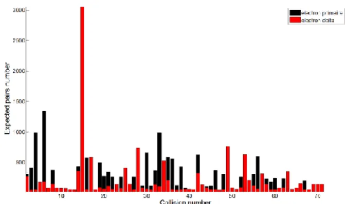
𝑛𝑗𝛿~𝒩( 𝑁𝑗𝛿, 𝐹𝑁𝑗𝛿) (4) As an illustration, Fig. 5 represents the series of expected numbers corresponding to the charge carrier pairs produced along the path of a 662 keV electron interacted with the pressurized xenon.
Fig. 5. Expected number of pairs of charge carriers produced for each collision number in the path of a primary electron of 662 keV (back) and for scattered δ electrons (red).
C. Charge carriers motion
Cylindrical coordinates are used to describe the ion chamber as presented in Fig. 6 where 𝑟𝑎 is the anode radius, 𝑟𝑐 is the cathode radius, 𝑟𝑔 is the radius of the Frisch grid and 𝑍 the height of the chamber.
Fig. 6. Geometrical model of the cylindrical ion chamber
The radial positions 𝜌𝑗,𝛼𝛿 associated to individual charges 𝛼 are generated based on a uniform distribution 𝑈 between two collisions (𝑗 = 1) or along the delta electron paths (𝑗 = 2) such as: ∀𝛼 ∈ [1; 𝑛1𝛿], ∀𝛿 ∈ [1; 𝑛𝛿], ∀𝑗 = {1; 2}, 𝜌𝑗,𝛼𝛿 = 𝑈 (√(𝑥𝑗,𝛼𝛿+1) 2 + (𝑦𝑗,𝛼𝛿+1)2, √(𝑥 𝑗,𝛼𝛿 ) 2 + (𝑦𝑗,𝛼𝛿 )2) (5) A current will be induced by the motion of each individual charge 𝛼 toward respective electrodes. The collection times 𝜏𝛼𝛿 required for charge 𝛼 to be collected are a random variable generated according to a normal law 𝒩 with an expectation 𝔼[𝜏𝛼𝛿 ] corresponding to the time of flight of the considered charge and with a variance 𝑉𝑎𝑟[𝜏𝛼𝛿 ] corresponding to a temporal-dispersion term. Indeed, thermal diffusion (Brownian motion) produces a Gaussian dispersion on arrival times whose variance is modeled by the Einstein-Smoluchowski formula. This dispersion is presented in Eq. 6-20 for electrons e and ions h where 𝑘𝐵 is the Boltzmann constant and 𝑇 is the temperature:
𝑣𝑒 𝔼[𝜏𝑗,𝛼,ℎ𝛿 ] = 𝑧𝑎− 𝑧𝑗,𝛼𝛿 𝑣ℎ (7) 𝑉𝑎𝑟(𝜏1,𝛼,𝑒𝛿 ) = 2𝑘𝐵𝑇(𝑧1,𝛼𝛿 − 𝑧𝑎)(𝑟𝑐− 𝑟𝑎) 𝑒𝑉 (8) 𝑉𝑎𝑟(𝜏1,𝛼,ℎ𝛿 ) = 2𝑘𝐵𝑇(𝑧𝑐− 𝑧1,𝛼𝛿 )(𝑟𝑐− 𝑟𝑎) 𝑒𝑉 (9) Charge carriers are susceptible to be trapped by impurities contained into the gas medium. Expected life-times 𝜃𝑒 and 𝜃ℎ of free charges in the gas are calculated according to Eq. 10– 11, where 𝛴𝑒 is the cross-section of electron captures, 𝛴ℎ is the cross section of ion captures and 𝐶𝑖 is the concentration of impurities. 𝜃𝑒= 𝑟𝑐− 𝑟𝑎 𝐶𝑖𝛴𝑒𝜇𝑒𝑉 (10) 𝜃ℎ= 𝑟𝑐− 𝑟𝑎 𝐶𝑖𝛴ℎ𝜇𝑒𝑉 (11) The life-time of individual charges is modeled by a random variable generated according to an exponential distribution ℇ with parameters 𝜃𝑒 and 𝜃ℎ. Effective collection times 𝜗𝛼𝛿 are estimated as the minimal value between motion duration and life expectation as seen in Eq. 12-13.
∀𝛼 ∈ [1; 𝑛1𝛿] & ∀𝛿 ∈ [1; 𝑛𝛿], ∀𝑗 = {1; 2},
𝜗𝑗,𝛼,𝑒𝛿 = 𝑚𝑖𝑛 {𝒩 (𝔼[𝜏𝑗,𝛼,𝑒𝛿 ], 𝑉𝑎𝑟(𝜏𝑗,𝛼,𝑒𝛿 )) ; ℇ(𝜃𝑒)} (12)
𝜗𝑗,𝛼,ℎ𝛿 = 𝑚𝑖𝑛 {𝒩 (𝔼[𝜏𝑗,𝛼,ℎ𝛿 ], 𝑉𝑎𝑟(𝜏𝑗,𝛼,ℎ𝛿 )) ; ℇ(𝜃ℎ)} (13)
During their motion, free charges will induce a current on the anode. Shockley-Ramo theorem allows the calculation of this current introducing a weighting field 𝜉𝑤 as described in Eq. 15. This field is obtained from the weighting potential gradient 𝜑𝑤 presented into the Poisson equation in Eq. 14 as a function of charge density ℵ and the dielectric permittivity 𝜀0𝜀𝑟. Equations are solved taking into account, as edge condition, a unit potential applied to the considered electrode (anode) and a null potential to the other electrode (𝑉(𝜌 = 𝑟𝑐) = 0 & 𝑉(𝜌 = 𝑟𝑎) = 1): ∇2𝜑 𝑤 = − ℵ 𝜀0𝜀𝑟 (14) 𝜉⃗𝑤 = −𝐠𝐫𝐚𝐝(𝜑𝑤) (15) Regarding charge motion phenomenon, the problem is invariant by rotation following the 𝜃 angle and by translation following the 𝑧 axis. The weighting field 𝜉𝑤 is finally calculated in Eq. 16 as a function of the radial position 𝜌 of a charge where 𝑟𝑐 and 𝑟𝑎 are the radius of the cathode and the anode:
𝑙𝑛 (𝑟
𝑎) 𝜌
Thanks to this weighting field, the currents induced by the electron and ion motion toward the electrodes 𝑖𝑒(𝑡) and 𝑖ℎ(𝑡) are obtained as functions of time 𝑡 ∈ ℝ+ such as:
∀𝛼 ∈ [1; 𝑛1𝛿], ∀𝛿 ∈ [1; 𝑛𝛿], ∀𝑗 = {1; 2}, ∀𝑡 ∈ [0; 𝜗𝑗,𝛼,𝑒𝛿 ], 𝑖𝑗,𝛼,𝑒𝛿 (𝑡) = 𝑒𝜉𝑤(𝑡)𝜇𝑒𝑉 𝑟𝑐− 𝑟𝑎 (17) = 𝑒𝜇𝑒𝑉 𝑙𝑛 (𝑟𝑐 𝑟𝑎) [(𝑟𝑐− 𝑟𝑎) 𝜌𝑗,𝛼 𝛿 − 𝜇 𝑒𝑉𝑡] ∀𝑡 ∈ [0; 𝜗𝑗,𝛼,ℎ𝛿 ], 𝑖𝑗,𝛼,ℎ𝛿 (𝑡) = 𝑒𝜉𝑤(𝑡)𝜇ℎ𝑉 𝑟𝑐− 𝑟𝑎 (18) = 𝑒𝜇ℎ𝑉 𝑙𝑛 (𝑟𝑐 𝑟𝑎) [(𝑟𝑐− 𝑟𝑎) 𝜌𝑗,𝛼 𝛿 + 𝜇 ℎ𝑉𝑡] ∀𝑡 ∈ [𝜗𝑗,𝛼,𝑒𝛿 ; +∞], 𝑖𝑗,𝛼,𝑒𝛿 (𝑡) = 0 (19) ∀𝑡 ∈ [𝜗𝑗,𝛼,𝑒𝛿 ; +∞], 𝑖𝑗,𝛼,ℎ𝛿 (𝑡) = 0 (20) In the presence of a Frisch grid, the current is solely induced on the anode when the electrons pass through the grid. The time for electron to achieve the grid 𝜏𝑔 and electronic and ionic currents 𝑖𝑗,𝛼,𝑒𝛿 (𝑡) , 𝑖𝑗,𝛼,ℎ𝛿 (𝑡) are presented in Eq. 21-23: 𝜏𝑔= ( 𝜌𝑗,𝛼𝛿 − 𝑟𝑔)(𝑟𝑐− 𝑟𝑎) 𝜇𝑒𝑉 (21) ∀𝜏𝑔> 0, ∀𝑡 ∈ [0; 𝜏𝑔], 𝑖𝑗,𝛼,𝑒𝛿 (𝑡) = 0 (22) ∀𝑡 ∈ [0; +∞], 𝑖𝑗,𝛼,ℎ𝛿 (𝑡) = 0 (23) When the electron reaches the grid, it can be trapped by the grid with a probability 𝑝𝑔 (typically 1%). A Bernoulli variable 𝑋 is set equal to 1 with a probability 𝑝𝑔 and 0 with a probability (1 − 𝑝𝑔). Finally, the signal resulting from charge collection is determined by summing the contribution of every elementary charge generated after each collision summed overall collisions. The electronic current, the ionic current and the total current are calculated as shown in Eq. 25-27:
𝑖𝑒(𝑡) = ∑ ∑ ∑ 𝑖𝑗,𝛼,𝑒𝛿 (𝑡) 𝑛1𝛿 𝛼=1 𝑛𝛿 𝛿=1 2 𝑗=1 (25) 𝑖ℎ(𝑡) = ∑ ∑ ∑ 𝑖𝑗,𝛼,𝑒𝛿 (𝑡) 𝑛1𝛿 𝛼=1 𝑛𝛿 𝛿=1 2 𝑗=1 (26) 𝑖(𝑡) = 𝑖𝑒(𝑡) + 𝑖ℎ(𝑡) (27)
D. Electronics
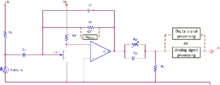
The detector is coupled to a charge sensitive preamplifier allowing the charge integration and delivering an output voltage which can be processed by analog or digital electronics (see Fig. 7).
Fig. 7. Schematic of front-end electronics
Charge integration is performed by the preamplifier whose time constant 𝜏𝑓 has to be high enough compared to the electron collection time 𝜏𝑒. Eq. 28-29 show the calculation of 𝜏𝑓 and 𝜏𝑒, where 𝑅𝑓 and 𝐶𝑓 are the feedback resistance and capacitance.
𝜏𝑒 = arg
𝑡 𝑚𝑖𝑛[𝑖𝑒(𝑡)] (28) 𝜏𝑓 = 𝑅𝑓𝐶𝑓 (29)
The equivalent signal charge 𝑄𝑠 is a function of the charge transfer efficiency 𝜂, which depends on the ratio between the detector capacitance 𝐶𝑑 and the FET gate source capacitance 𝐶𝑔𝑠. Eq. 30 details the calculation of the detector capacitance as a function of the absolute and relative dielectric constant 𝜀0 and 𝜀𝑟 in the cylindrical detector:
𝐶𝑑=
2𝜋𝜀0𝜀𝑟𝑍 𝑙𝑛 (𝑟𝑐
𝑟𝑎)
(30) The calculation of the charge transfer efficiency 𝜂 is detailed in Eq. 31:
𝜂 = 1
1 + 𝐶𝑑 𝐶𝑔𝑠
(31)
The current from the detector is integrated by the preamplifier and then differentiated to obtain a differential output current 𝑖𝑑(𝑡) as shown in Eq. 34. The integration and differentiation impulse responses ℎ𝑖(𝑡) and ℎ𝑑(𝑡) are presented in the Eq. 32-33, where 𝜏𝑑 is the time constant of the differentiator circuit (𝜏𝑑≪ 𝜏𝑓).
ℎ𝑖(𝑡) = 1 𝜏𝑓𝑒𝑥𝑝(− 𝑡 𝜏⁄ ) (32) 𝑓 ℎ𝑑(𝑡) = 𝛿(𝑡) − 1 𝜏𝑑𝑒𝑥𝑝(− 𝑡 𝜏⁄ ) (33)𝑑 𝑖𝑑(𝑡) = 𝜂 ((𝑖 ∗ ℎ𝑖) ∗ ℎ𝑑)(𝑡) (34)
The signal can be processed by an analog or digital circuit. The first strategy regarding the triggering optimization and SNR maximization is the implementation of a linear shaping filter with a triangular impulse response ℎ𝑠(𝑡) presented in Eq. 35. This filter is close to the optimal cups filter and it is then largely implemented into analog and digital electronics [9, 10]. It is defined by the zeros-to-peak time constant 𝜏𝑚 such as: ℎ𝑠(𝑡) {= 1 − |𝑡| 𝑡𝑚 ∀𝑡 ∈ [−𝑡𝑚; 𝑡𝑚] = 0 ∀𝑡 ∈ [−∞; −𝑡𝑚[ ∪ [𝑡𝑚; +∞] (35) The equivalent output current 𝑖𝑠(𝑡) obtained by this filtering is described in Eq. 36.
𝑖𝑠(𝑡) = (𝑖𝑑∗ ℎ𝑠)(𝑡) (36) Finally, the equivalent source charge 𝑄̂𝑠 is estimated by the maximum of the equivalent output current 𝑖𝑠(𝑡) which is an estimation of the deposited energy 𝐸0 where 𝑘 is a calibration factor.
𝐸̂0= 𝑘 𝑄̂𝑠= 𝑘 𝑚𝑎𝑥(𝑖𝑠(𝑡)) (37) On the other hand, Digital Signal Processing unit (DSP) allows the implementation of nonlinear filtering approaches. These methods are able to maximize the SNR as efficiently as linear filters without any pulse shaping [11, 12]. The equivalent output current 𝑖𝑑(𝑡) is filtered into an anti-aliasing analog circuit before its digitalization thanks to an Analog to Digital Convertor (ADC). The estimated charge 𝑄̂𝑠′ is therefore obtained by a simple integration of equivalent current pulse 𝑖𝑑(𝑡) as presented in Eq. 38. 𝐸̂0= 𝑘 𝑄̂𝑠′= 𝑘 ∫ 𝑖𝑑(𝑡) +∞ 𝑡=0 𝑑𝑡 (38)
Thanks to the high bandgap of noble gases, the leakage current induced by thermal production of free-charges can be considered as null (𝑒𝑥𝑝(− 𝐸𝑔⁄𝑘𝐵𝑇) = 2. 10−174). The noise arising from the insulator surface and the noise coming from electromagnetic compatibility (EMC) are considered as environmental perturbations and are not deal with in this study. The digital noise (quantification and sampling) induced by the DSP is also considered as null as it is not a challenge with currently available ADC [13]. It is then considered that the major part of the electronic noise comes from electronic components located at the first stage of the preamplifier. Indeed, the electronic noise can be divided in two parts: a parallel noise and a serial noises:
Parallel noise is the noise induced by components set in parallel with regards to the preamplifier entrance. It is itself composed by Johnson-Nyquist noises thermally induced into the bias and the feedback resistances (𝑅𝑏 and 𝑅𝑓 respectively);
calculated as presented in the Eq. 39: 𝐸𝑁𝐶𝑝2= [ 1.34 𝑘𝐵𝑇(𝑅𝑓+ 𝑅𝑏) 𝑅𝑓𝑅𝑏 + 2𝑒𝑉𝑏 𝑅𝑏 ] 𝜏𝑚 (39) The contribution of this noise decreases when the bandwidth increases. It has to be maintained as low as possible by setting the parallel resistors at very high values. This requirement follows the same direction as the necessity to ensure full charge integration (ensured by 𝜏𝑓 ≫ 𝜏𝑒), but roses the risk of preamplifier saturation when the pulse rate increases. The electron collection time is especially high in large gas chambers, which imposes to implement high value for the feedback resistance. The use of transistor reset preamplifiers is a more efficient way to operate with a quasi-infinite feedback resistance and managing of the saturation phenomenon. The parallel noise could then be considered as low compared to the serial noise contribution 𝐸𝑁𝐶𝑝2≪ 𝐸𝑁𝐶𝑠2.
The serial noise arises from a thermal leakage current into the FET itself and a flicker noise (ie. 1/f noise). The equivalent noise charge from serial noise 𝐸𝑁𝐶𝑠 is calculated as presented in Eq. 40 where 𝑔𝑚 is the transconductance and 𝐾𝑓 the flicker noise constant of the FET component:
𝐸𝑁𝐶𝑠2= (𝐶𝑑+ 𝐶𝑔𝑠) 2 [8𝑘𝐵𝑇 3𝑔𝑚𝜏𝑚+ 𝐾𝑓 𝐶𝑔𝑠] (40) The FET has to be chosen with a high transconductance 𝑔𝑚 (5 mS) and low flicker energy constant 𝐾𝑓 (10-27 J). A compromise has to be made with regards to the gate-source capacitance. Indeed, high values increase the charge transfer efficiency 𝜂, but also the serial noise contribution. Matching by 𝐶𝑑≈ 𝐶𝑔𝑠 allows an optimization to be made. The thermal part of the serial noise increases with the bandwidth, whereas the flicker part is independent from it. In linear filters, the time constant 𝑡𝑚 has to be set large enough to decrease the thermal noise under the flicker noise level. However, the system dead time will increase dramatically with the shaping time constant increasing. Nonlinear filtering implementable into DSP then constitute a better strategy to deal with SNR maximization without any pulse shaping.
The noise charge 𝑄𝑛 is calculated using the total equivalent noise charge as a standard deviation of a normal law as shown in Eq. 41.
𝑄𝑛~ 𝒩 (0, √𝐸𝑁𝐶𝑝2+ 𝐸𝑁𝐶𝑠2) (41)
III. RESULTS
parameters.
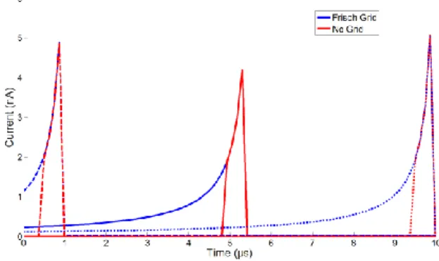
Interaction of a 662 keV photon into an HPXe chamber is simulated by MCNPX and the processing of the output PTRAC file is subsequently run. An example of the current induced by the charge carriers at the anode is presented in Fig 6. We can observe that the Frisch grid reduces the dependence on the interaction location.
Fig. 8. Example of pulse shape 𝑖𝑑(𝑡) measured at the output of the
preamplifier, close to the anode (long dash line), between anode and cathode (full line) and close to the cathode (small dash line).
The signal measured at the output of the shaper is shown in Fig. 9.
Fig. 9. Example of pulse shape 𝑖𝑠(𝑡) measured at the output of the shaper,
close to the anode (long dash line), between anode and cathode (full line) and close to the cathode (small dash line).
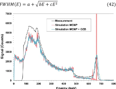
A gamma spectrum has been measured with an HPXe chamber filled with a xenon density of 0.25 g.cm-3 (0.3 % H2, 113 mm diameter and 170 mm length). The measure has been simulated by MCNPX code in order to produce the related PTRAC file. The measured spectrum and the deposited energy spectrum (tally f8) obtained by simulation are shown in Fig. 10. Simulated and experimental spectra show a relatively good accordance proving that the physics of the interaction is well processed in MCNPX code. The lack of counts at low energy could be explained by the fact that all scattered photons are not taken into account in the current version of our model. A Gaussian broadening card (GEB card) has been implemented in order to match the simulation with the experiment adding an artificial resolution. We should notice here that the parameter a b c of the Gaussian broadening (see Eq. 42) could only be set a posteriori with regards to the experimental observation.
𝐹𝑊𝐻𝑀(𝐸) = 𝑎 + √𝑏𝐸 + 𝑐𝐸2 (42)
Fig. 10. Gamma spectrum obtained for an HPXe chamber with a xenon density of 0.25 g.cm-3 (0.3 % H
2, 113 mm diameter and 170 mm length). Fig. 11 shows the pulse high spectrum obtained thanks to the computation of the PTRAC file by the pulse model simulation presented above. The blue spectrum is the spectral response with the intrinsic resolution of the detector where only the statistical fluctuation of charge carrier number is taken into account). The green spectrum is the spectral response with intrinsic resolution and dispersions due to charge motion effects as charge recombination, grid trapping, thermal diffusion and ion motion toward to cathode. The Frisch grid allows a robust limitation of the resolution discrepancy thanks to the shielding of the ionic part of the signal. The electronic noise is finally added and the red spectrum represents the signal as it can be measured by such a detector. It can be seen that this final spectrum is close to the experimentally obtained one. This result constitutes a first validation of the full detector simulation.
Fig. 11. Gamma spectrum obtained for an HPXe chamber with a xenon density of 0.25 g.cm-3 (0.3 % H2, 113 mm diameter and 170 mm length).
IV. DISCUSSION
As individual pulses can be simulated, it is now possible to simulate the temporal series of interaction events. The general model is presented in Eq. 43 for a series of pulses 𝑘 where 𝑖𝑠𝑘(𝑡) is the temporal shape of individual pulse and 𝜏𝑘 the inter-pulses period. The period 𝜏𝑘 is calculated in Eq. 44 by sampling an exponential distribution ℇ with an expected inter-pulse period 𝑇.
𝑗𝑠(𝑡) = ∑ 𝑖𝑠𝑘(𝑡 − 𝜏𝑘) 𝑘>1
(43) 𝜏𝑘~ℇ(𝑇) (44) Traditionally the temporal signal is simulated without taking into account the individual shape of the stochastic pulse series. The pulse is decomposed in charge amplitude 𝑄𝑘 and a general model for the pulse impulse response 𝐻(𝑡) as seen in Eq. 45.
𝑖𝑠𝑘(𝑡) = 𝑄𝑘𝐻(𝑡) (45) Therefore, the signal could be simulated in a better way in Eq. 43 in order to study pile-up or fluctuation phenomena [14]. This implementation will be explored in future works.
V. CONCLUSION
A model allowing the simulation of the overall ion chamber detector has been described. MCNPX simulation has been completed by the processing of the output PTRAC file. At each individual interaction, the production and the migration of the charge carriers has been simulated to format every individual pulse shape. The associated electronic noise has also been taken into account according to electronic parameters of the detector and front-end electronics.
The simulation has been compared with experimental data obtained by an HPXe chamber prototype. The good agreement between experimental and simulation constitute a first validation of this simulation technique applied to radiation detectors. This approach gives the opportunity to optimize both physical and electronics parameters for R&D in the field of nuclear instrumentation.
REFERENCES
[1] M. Kurokawa, S. Shimoura, H. Iwasaki, H. Baba, S. Michimasa, S. Ota, H. Murakami and H. Sakai, “Pulse Shape Simulation and Analysis of Segmented Ge Detectors for Position Extraction.” IEEE Transactions on Nuclear Science, 50(5): 1309-1316, 2003.
[2] I. Abt, A. Cadwell, D. Lenz, J. Liu, X. Liu, and B. Majorovits, “Pulse shape simulation for segmented
true-[3] M. Schlarb, R. Gernhäuser, S. Klupp, and R. Krücken, “Pulse shape analysis for γ-ray tracking: Pulse shape simulation with JASS.” The European Physical Journal A 47: 132, 2011.
[4] P. Filliatre, C. Jammes, B. Geslot, and R. Veenhof, “A Monte Carlo simulation of the fission chambers neutron-induced pulse shape using the GARFIELD suite.” Nuclear
Instruments and Methods in Physics Research A 678: 139–
147, 2012.
[5] J. Mock, N. Barry, K. Kazkaz, D. Stolp, M. Szydagis, M. Tripathi, S. Uvarov, M. Woods, N. Walsh. “Modeling Pulse Characteristics in Xenon with NEST.” Journal of
Instrumentation 9, T04002, 2014.
[6] G.W. McKinney, et al. “MCNPX 2.7.0 New Features Demontrated” – Los Alamos National Laboratory technical report LA-UR-12-25775, 2012.
[7] V.V. Dmitrenko, A.S. Romanyuk, S.I. Suchkov, and Z.M. Uteshev. Electron mobility in dense xenon gas. Soviet
Physics Technical Physics, 28:1440–1444, 1983.
[8] A. Bolotnikov and B. Ramsey. The spectroscopic properties of high-pressure xenon. Nuclear Instruments and
Methods in Physics Research A, 396:360–370, 1997.
[9] V. Radeka. “ Low-noise techniques in detectors.” Annual
Reviews of Nuclear and Particle Science 38: 217-277, 1988.
[10] V.T. Jordanov, G.F. Knoll, A.C. Huber and J.A. Pantazis. “Digital techniques for real-time pulse shaping in radiation measurements “. Nuclear Instruments and Methods in Physics
Research A 353 261-264, 1994.
[11] E. Barat, T. Dautremer, T. Montagu and J-C. Trama. “A bimodal Kalman smoother for nuclear spectrometry”. Nuclear
Instruments and Methods in Physics Research A 353 261-264,
1994.
[12] Y. Moline, M. Thevenin, G. Corre and M. Paindavoine. “Auto-Adaptive Trigger and Pulse Extraction for Digital Processing in Nuclear Instrumentation”. IEEE Transaction on
Nuclear Science, submitted 2015.
[13] S. Normand, et. al. “PING for Nuclear Measurements: First Results”, IEEE Transactions on Nuclear Science, 59(4): 1232-1236, 2012.
[14] T. Rebafka, F. Roueff and A. Souloumiac. “Information bounds and MCMC parameter estimation for the pile-up model”. Journal of Statistical Planning and Inference, 141: 1– 16, 2011.