Covariation of climate and long-term erosion rates across
a steep rainfall gradient on the Hawaiian island of Kaua'i
The MIT Faculty has made this article openly available. Please share how this access benefits you. Your story matters.
Citation Ferrier, K. L., J. T. Perron, S. Mukhopadhyay, M. Rosener, J. D. Stock, K. L. Huppert, and M. Slosberg. “Covariation of Climate and Long-Term Erosion Rates Across a Steep Rainfall Gradient on the Hawaiian Island of Kaua’i.” Geological Society of America Bulletin 125, no. 7–8 (July 1, 2013): 1146–1163.
As Published http://dx.doi.org/10.1130/B30726.1
Publisher Geological Society of America
Version Author's final manuscript
Citable link http://hdl.handle.net/1721.1/85607
Terms of Use Creative Commons Attribution-Noncommercial-Share Alike Detailed Terms http://creativecommons.org/licenses/by-nc-sa/4.0/
1
Covariation of climate and long-term erosion rates across a
1steep rainfall gradient on the Hawaiian island of Kaua‘i
23
Ken L. Ferrier1, J. Taylor Perron1, Sujoy Mukhopadhyay2, Matt Rosener3,
4
Jonathan D. Stock4, Kimberly L. Huppert1, Michelle Slosberg1
5
1 Department of Earth, Atmospheric, and Planetary Sciences, Massachusetts Institute of
6
Technology, Cambridge, MA
7
2 Department of Earth and Planetary Sciences, Harvard University, Cambridge, MA
8
3 U.S. Geological Survey, Hanalei, Kaua‘i, HI
9
4 U.S. Geological Survey, Menlo Park, CA
10 11
ABSTRACT
12
Erosion of volcanic ocean islands creates dramatic landscapes, modulates Earth’s 13
carbon cycle, and delivers sediment to coasts and reefs. Because many volcanic islands 14
have large climate gradients and minimal variations in lithology and tectonic history, they 15
are excellent natural laboratories for studying climatic effects on the evolution of 16
topography. Despite concerns that modern sediment fluxes to island coasts may exceed 17
long-term fluxes, little is known about how erosion rates and processes vary across island 18
interiors, how erosion rates are influenced by the strong climate gradients on many 19
islands, and how modern island erosion rates compare to long-term rates. Here we 20
present new measurements of erosion rates over 5-year to 5-million-year timescales on 21
the Hawaiian island of Kaua‘i, across which mean annual precipitation ranges from 0.5 to 22
2 9.5 m/yr. Eroded rock volumes from basins across Kaua‘i indicate that Myr-scale
23
erosion rates are correlated with modern mean annual precipitation and range from 8 to 24
335 t km-2 yr-1. In Kaua‘i’s Hanalei River basin, 3He concentrations in detrital olivines 25
imply millennial-scale erosion rates of >126 to >390 t km-2 yr-1 from olivine-bearing 26
hillslopes, while fluvial suspended sediment fluxes measured from 2004 to 2009 plus 27
estimates of chemical and bedload fluxes imply basin-averaged erosion rates of 545 ± 28
128 t km-2 yr-1. Mapping of landslide scars in satellite imagery of the Hanalei basin from 29
2004 and 2010 imply landslide-driven erosion rates of 30-47 t km-2 yr-1. These 30
measurements imply that modern erosion rates in the Hanalei basin are no more than 2.3 31
± 0.6 times faster than millennial-scale erosion rates, and, to the extent that modern 32
precipitation patterns resemble long-term patterns, they are consistent with a link between 33
precipitation rates and long-term erosion rates. 34
35
INTRODUCTION
36
A glance at a topographic map of the Hawaiian Islands makes it clear that a great 37
deal of rock is eroded from volcanic islands over time (e.g., Dana, 1890). The recently 38
erupted lava flows on Mauna Loa and Kilauea volcanoes on the Island of Hawai‘i form 39
smooth hillslopes that are undissected by rivers, and they stand in stark contrast to older 40
Hawaiian islands like Kaua‘i, which over the past >4 Myr has been dissected by canyons 41
more than 1 km deep. The dramatic erosion of island interiors and the correspondingly 42
large sediment fluxes to coasts are not unique to the Hawaiian Islands, but instead are 43
common features of many ocean islands, such as the Society Islands (e.g., Hildenbrand et 44
3 al., 2008), the Lesser Antilles (e.g., Rad et al., 2007), and Iceland (e.g., Louvat et al., 45
2008). 46
The erosion of volcanic islands offers an opportunity to investigate a number of 47
problems central to landscape evolution. For instance, islands are isolated from 48
continents and thus offer opportunities to investigate the co-evolution of topography and 49
biota (e.g., Craig, 2003). Because islands are small, they offer an opportunity to study 50
how boundary effects propagate through landscapes. Volcanic islands are also well 51
suited for isolating climatic effects on erosion, because many islands exhibit large spatial 52
variations in climate but relatively small variations in non-climatic factors that might also 53
affect erosion rates, such as lithology and tectonic deformation. This is particularly 54
valuable because the effects of climate on erosion rates are a matter of long-standing and 55
continuing debate (e.g., Langbein and Schumm, 1958; Riebe et al., 2001; DiBiase and 56
Whipple, 2011), and because attempts to measure climatic effects on erosion rates are 57
often confounded by site-to-site variations in non-climatic factors (e.g., Walling and 58
Webb, 1983; von Blanckenburg, 2005). Furthermore, climate’s effect on erosion rates is 59
often cited as the driver for an important feedback in the co-evolution of climate, 60
topography, and mountain structure (e.g., Willett, 1999; Beaumont et al., 2001; Whipple 61
and Meade, 2004; Stolar et al., 2007; Roe et al., 2008; Whipple, 2009), and despite a few 62
observations of correlations between precipitation rates and erosion rates (e.g., Reiners et 63
al., 2003; Owen et al., 2010; Moon et al., 2011), there remains no empirical consensus on 64
the net effects of climate on erosion rates. Lastly, volcanic islands are examples of 65
transient landscapes, with topography that is lowered by both surface erosion and island 66
subsidence. This distinguishes islands from many continental settings in which rock 67
4 uplift counterbalances erosion, driving the topography toward an approximate steady 68
state (e.g., Hack, 1960). Such transiently evolving landscapes are valuable because their 69
morphologies can be more sensitive indicators of erosional processes than steady-state 70
landscapes, which makes transient landscapes better suited for evaluating proposed 71
models of landscape evolution (e.g., Tucker and Whipple, 2002; Tucker, 2009). 72
Furthermore, climatic effects on erosion rates should be more apparent in transient 73
landscapes than in steady-state landscapes, because erosion rates are governed by rock 74
uplift rates in steady-state landscapes. 75
Volcanic islands thus have the potential to reveal much about landscape 76
dynamics, and therefore have implications for continental topography as well as island 77
topography, because erosional processes in many continental regions are similar to those 78
on volcanic islands (e.g., Lohse and Dietrich, 2005; Jefferson et al., 2010). Yet, despite 79
widespread attention to sediment fluxes along island coasts, comparatively little is known 80
about how the interiors of ocean islands erode and how the dominant erosional processes 81
and rates vary in space and time. For instance, in a study of Kaua‘i’s Waimea basin, 82
Gayer et al. (2008) measured a 10-fold variation in cosmogenic 3He concentrations 83
among 26 samples of detrital olivine collected from a single site near the basin outlet. 84
They suggested that this variation was best explained by spatially variable erosion rates 85
driven by a nonlinear dependence of erosion rates on hillslope gradient. Without 86
systematic measurements of erosional processes and rates in island interiors, it will be 87
difficult to take full advantage of these natural experiments in landscape evolution. 88
The importance of such studies is augmented by societal concerns over sediment 89
fluxes to coral reefs, where excessive sediment supply can smother reefs, reduce coral 90
5 calcification and tissue growth, inhibit larval recruitment, and restrict light from
91
photosynthetic algae (e.g., Rogers, 1979; 1990; Cox and Ward, 2002; Telesnicki and 92
Goldberg, 1995; Yentsch et al., 2002, Fabricius, 2005). This is a growing concern 93
because coral reefs around the world are in rapid decline: recent surveys report that 94
nearly 60% of global reefs may disappear by 2030 (Wilkinson, 2002; Gardner et al., 95
2003). To properly manage reefs, it is vital to know the long-term average rates of 96
sediment delivery to coasts and to determine how those rates may have changed under 97
human activity. This in turn requires erosion rate measurements over a range of 98
timescales at a single location, ideally combined with an inventory of the erosional 99
processes that are responsible for generating sediment. 100
Prior studies of steep hillslopes on the Hawaiian Islands suggest that hillslope 101
erosion proceeds by a combination of soil creep (Wentworth, 1943; White, 1949; Scott, 102
1969; Scott and Street, 1976), shallow landslides in the soil (Wentworth, 1943; Ellen et 103
al., 1993), landslides with failure in the saprolite (Peterson et al., 1993), bedrock 104
avalanches (Jones et al., 1984), debris flows (Hill et al., 1997), and flushing of solutes 105
(Moberly, 1963; Li, 1988). Special attention has been paid to the role of shallow 106
landslides, since field observations of abundant landslide scars suggest that shallow 107
landslides may be responsible for a large fraction of the mass flux from hillslopes to 108
channels in steep Hawaiian basins (Wentworth, 1943; Scott, 1969; Ellen et al., 1993; 109
Peterson et al., 1993). Quantifying sediment fluxes due to landslides may therefore be of 110
central importance in sediment budgets for volcanic islands. 111
In this paper, we use Kaua‘i as a natural laboratory for addressing three questions 112
central to the erosion of volcanic islands. First, how do precipitation rates affect erosion 113
6 rates on volcanic islands, and how do erosion rates vary spatially as a result? Second, 114
how do modern erosion rates on volcanic islands compare to erosion rates over million-115
year and millennial timescales? Third, how important is shallow landsliding in setting 116
erosion rates on volcanic islands? Kaua‘i is well suited for this study because it exhibits 117
minimal variations in lithology while spanning one of Earth’s steepest regional rainfall 118
gradients, with annual rainfall rates ranging from 0.5 m/yr to 9.5 m/yr over only 25 km. 119
To address these questions we present four new sets of erosion rate measurements on 120
Kaua‘i, inferred from (1) the volumetric excavation of basins since the formation of the 121
volcano surface; (2) 3He concentrations in olivine grains collected in river sediment; (3) 122
modern fluvial sediment fluxes; and (4) modern landslide inventories. We focus 123
particular attention on Kaua‘i’s Hanalei basin because previous work on sediment fluxes 124
there provides a context for our new measurements (e.g., Calhoun and Fletcher, 1999; 125
Draut et al., 2009; Takesue et al., 2009; Stock and Tribble, 2010), and because sediment 126
from the Hanalei River discharges into Hanalei Bay, where high turbidity is an ecological 127
concern (EPA, 2008; Hawaii Department of Health, 2008). In the following pages we 128
introduce the study area on Kaua‘i, describe the methods we used to measure erosion 129
rates, and discuss the implications of spatial and temporal variations in the measured 130
erosion rates. 131
132
KAUA‘I GEOLOGY, TOPOGRAPHY, AND CLIMATE
133
Kaua‘i is the northernmost and second oldest major extant Hawaiian island. Like 134
the other Hawaiian islands, Kaua‘i is a product of hotspot volcanism. Over 95% of 135
Kaua’i’s rock volume consists of tholeiitic basalt, which erupted during Kaua‘i’s shield-136
7 building stage 5.1-4.0 Ma and which is classified into the Na Pali Member, the Olokele 137
Member, the Makaweli Member, and the Haupu Member (Figure 1; McDougall, 1979; 138
Clague and Dalrymple, 1988; Garcia et al., 2010). After more than one million years of 139
quiescence, a second stage of episodic volcanism began at ~2.6 Ma and lasted to 0.15 140
Ma, over which time alkalic basalts mantled about half the island (Figure 1; Garcia et al., 141
2010). These so-called rejuvenated lavas constitute the second major stratigraphic group 142
on Kaua‘i, and are known collectively as the Koloa volcanics. 143
Unlike some younger volcanic islands, Kaua‘i has experienced major structural 144
deformation since the growth of its initial shield, including collapse of the Olokele 145
Caldera near the center of the island, dropdown of the Makaweli graben in the 146
southwestern part of the island, and formation of the Lihue basin on the eastern side of 147
the island (Macdonald et al., 1960). Some studies have suggested that Kaua‘i is not a 148
single shield volcano but rather a composite of two shield volcanoes, on the basis of 149
patterns in submarine rift zones and differences in Sr, Nd, and Pb isotopic compositions 150
in basalts on the east and west sides of Kaua‘i (Clague, 1996; Holcomb et al., 1997; 151
Mukhopadhyay et al., 2003). 152
Kaua‘i’s complex structural history is reflected in its topography. The eastern 10-153
15 km of the island is dominated by the low-lying Lihue basin, which is interpreted to 154
have formed by structural collapse rather than by fluvial erosion (Reiners et al., 1998). 155
By contrast, the western 5-10 km of the island is dominated by short, narrow, steep-sided 156
canyons incised into the Na Pali Member, and is interpreted as a fluvially dissected 157
remnant of Kaua‘i’s earliest shield surface (Figure 1). Between the eastern and western 158
sides of the island stands the Olokele plateau, which is composed of nearly horizontal 159
8 caldera-filling lavas, and which has been incised with several canyons over 1 km deep 160
(Macdonald et al., 1960). 161
Kaua‘i’s climate is strongly affected by its topography. During most of the year, 162
trade winds blow from the northeast and are forced up the east-facing Wai‘ale‘ale 163
escarpment near the center of the island. The rising air is confined near the island’s 164
summit at 1593 m by a subsidence inversion at an elevation of 1.8-2.7 km (Ramage and 165
Schroeder, 1999), which forces the air to drop much of its moisture at the summit. This 166
produces a bulls-eye pattern in mean annual rainfall rates over the island, with high 167
rainfall rates at the island’s center and low rainfall rates at the coast, superimposed upon a 168
regional gradient with higher rainfall rates in the upwind northeastern half of the island 169
than in the downwind southwestern half (Figure 2; PRISM Climate Group, Oregon State 170
University). This results in one of the largest and steepest rainfall gradients on Earth. 171
Rainfall rates between 1949 and 2004 on Mt. Wai‘ale‘ale near the island’s center 172
averaged 9.5 m/yr – among the highest on Earth – while rainfall rates between 1949 and 173
2000 on the southwestern part of the island, just 25 km away, averaged 0.5 m/yr (Western 174
Regional Climate Center). Given that a precipitation rate of 12.7 m/yr in Lloro, Colombia 175
is often cited as the highest on Earth (e.g., Poveda and Mesa, 2000), the range of rainfall 176
rates across Kaua‘i represents >70% of the range in rainfall rates on Earth. The wide 177
range in rainfall rates and minimal variations in lithology make Kaua‘i an excellent 178
natural laboratory for investigating the effects of rainfall rates on erosion rates. 179
180
METHODS: CALCULATING EROSION RATES
181
Million-year erosion rates inferred from basin excavation and bedrock age
9 A common method for estimating basin-averaged erosion rates EV (M L-2 T-1) is
183
to measure the volume V of material of density ρr eroded from a basin of area Ab over a
184
given time interval Δt, as in Equation 1. 185
!
EV = "rV
Ab#t (1)
186
If the time interval Δt is taken to be the time between the construction of the initial 187
topography and the present, this technique requires accurate estimates of the initial 188
topography, the present topography, and the timing of the onset of erosion. This 189
approach is amenable to application on young volcanic islands, because uneroded 190
remnants of the volcano surface permit reconstruction of the pre-erosional volcano 191
topography, and because many volcanic rocks are suitable for radiometric dating (e.g., 192
Wentworth, 1927; Li, 1988; Ellen et al., 1993; Seidl et al., 1994; Hildenbrand et al., 193
2008). 194
Portions of Kaua‘i are suitable for such an approach. The western flank of Kaua‘i 195
along the Na Pali Coast and above the Mana Plain, for example, is dissected with 196
numerous drainage basins that are short (4-10 km from headwaters to outlet) and narrow 197
(1-2 km wide). Rivers have incised narrow canyons into the centers of many of these 198
drainage basins, and they have left relatively planar, minimally dissected topographic 199
surfaces standing above and between many of the canyons, dipping toward the coast at 200
gradients of 4-6°. The bedrock in this region is basalt of the Na Pali Formation, which is 201
considered to be the remnant flank of Kaua‘i’s first volcanic edifice, and, with a K-Ar 202
age of 4.43 ± 0.45 Ma, is the oldest dated bedrock on Kaua‘i (McDougall, 1979). 203
We used the minimally eroded interfluve surfaces in a 10-m digital elevation map 204
(US National Elevation Dataset) to constrain the pre-erosional topography of each basin 205
10 along Kaua‘i’s western flank, similar to the approach that Seidl et al. (1994) and Stock 206
and Montgomery (1999) used to estimate the vertical extent of river incision in the same 207
region of Kaua‘i. For each basin, we constructed a model of the pre-erosional 208
topography in two steps. First, we mapped the topography around the basin’s perimeter, 209
including all neighboring remnants of minimally eroded topography and the basin 210
ridgelines between the minimally eroded remnants. We then fit a thin-plate smoothing 211
spline (with smoothing parameter p = 1, corresponding to a natural cubic spline) across 212
the basin, fixing the edges of the spline surface to the mapped topography around the 213
basin’s perimeter. Because the elevation of mapped perimeter may be as high as the 214
initial topography but no higher, we consider the spline surface fit to the mapped 215
perimeter to be a minimum bound on the elevation of the pre-erosional topography. We 216
then subtracted the present topography from the initial topography to calculate the rock 217
volume eroded from the basin, divided the eroded volume by the basin area and the age 218
of the bedrock, and multiplied by an assumed rock density of ρr = 3 g/cm3 to calculate a
219
basin-averaged erosion rate (Equation 1; Table 1; Figure 2). We assume, in Equation 1, 220
that uncertainties in drainage area, eroded volume, and bedrock density are negligible 221
relative to the uncertainties in bedrock age (Table 1). This calculation does not include 222
potential variations in basalt porosity, which would lower the bulk rock density and hence 223
estimates of EV.
224 225
Table 1: Basin-averaged erosion rates determined from rock volumes eroded since 226
construction of the basin’s initial surface (Equation 1). ID refers to basin 227
identification numbers in Figure 2. Values for mean annual precipitation (MAP) 228
11 are basin averages (Daly et al., 2002; PRISM Climate Group). Bedrock ages for 229
lithologic units are: Na Pali formation 4.43 ± 0.45 Ma (McDougall, 1979); 230
Olokele formation 3.95 ± 0.05 Ma (Clague and Dalrymple, 1988); Makaweli 231
formation 3.91 ± 0.01 Ma (Clague and Dalrymple, 1988; Garcia et al., 2010); and 232
Koloa volcanics in the Hanalei basin 1.50 ± 0.12 Ma (Clague and Dalrymple, 233 1988; Garcia et al., 2010). 234 235 Basin ID Area Ab (km2) Eroded volume
V (km3) Bedrockage (Ma) MAP (mm/yr)
Fraction fV of initial volume eroded (%) Erosion rate EV (t km-2 yr-1) Mana/Na Pali Awa‘awapuhi 1 2.70 0.154 4.43 ± 0.45 1337 5 36 ± 4 Haeleele 2 5.64 0.362 4.43 ± 0.45 1189 9 43 ± 4 Hanakapi‘ai 3 9.58 1.761 4.43 ± 0.45 3071 20 124 ± 13 Hanakoa 4 4.92 0.464 4.43 ± 0.45 2286 10 64 ± 6 Hikimoe 5 5.59 0.268 4.43 ± 0.45 1245 6 29 ± 3 Hoea 6 19.46 0.910 4.43 ± 0.45 841 8 30 ± 3 Honopu 7 3.29 0.613 4.43 ± 0.45 1187 20 124 ± 12 Huluhulunui 8 1.51 0.027 4.43 ± 0.45 639 7 11 ± 1 Kaawaloa 9 8.22 0.357 4.43 ± 0.45 918 7 29 ± 3 Kaaweiki 10 4.49 0.273 4.43 ± 0.45 1157 8 35 ± 4 Kahelunui 11 6.46 0.265 4.43 ± 0.45 913 6 25 ± 3 Kahoaloha 12 6.23 0.257 4.43 ± 0.45 1111 5 26 ± 3 Kalalau 13 10.45 3.633 4.43 ± 0.45 1479 33 217 ± 22 Kapilimao 14 4.13 0.129 4.43 ± 0.45 668 10 21 ± 2 Kauhao 15 7.62 0.793 4.43 ± 0.45 1280 12 64 ± 7 Ka‘ula‘ula 16 5.26 0.254 4.43 ± 0.45 1153 6 29 ± 3 Kuapa‘a 17 3.45 0.105 4.43 ± 0.45 707 9 21 ± 2 Makaha 18 6.40 0.477 4.43 ± 0.45 1269 8 44 ± 4 Miloli‘i 19 9.26 0.522 4.43 ± 0.45 1267 5 26 ± 3 Nahomalu 20 9.97 0.356 4.43 ± 0.45 1038 5 24 ± 2 Niu 21 2.83 0.108 4.43 ± 0.45 752 10 26 ± 3 Nu‘alolo 22 6.42 0.536 4.43 ± 0.45 1290 11 66 ± 7 ‘Ohai‘ula 23 4.96 0.146 4.43 ± 0.45 899 6 20 ± 2 Paua 24 1.92 0.023 4.43 ± 0.45 654 5 8 ± 1 Wai‘aka 25 3.88 0.104 4.43 ± 0.45 688 8 17 ± 2 Wailao 26 3.15 0.110 4.43 ± 0.45 752 9 26 ± 3 Waipao 27 4.42 0.142 4.43 ± 0.45 720 8 22 ± 2 Large basins Hanalei 28 60.04 11.69 – 1.50 ± 0.12, 3866 32 – 42 175 – 309
12 23.58 3.95 ± 0.05, 4.43 ± 0.45 Hanalei (east) 21.42 1.56 1.50 ± 0.12, 4.43 ± 0.45 3301 19 146 ± 12 Hanalei (west) 38.62 10.13-22.02 3.95 ± 0.05, 4.43 ± 0.45 4179 39 – 55 192 – 400 Hanapepe 29 67.83 13.28 3.95 ± 0.05, 4.43 ± 0.45 2897 29 133 ± 13 Lumahai 30 35.63 15.78 3.95 ± 0.05, 4.43 ± 0.45 3716 45 335 ± 4 Makaweli 31 68.70 13.39 3.91 ± 0.01, 3.95 ± 0.05, 4.43 ± 0.45 2961 21 121 ± 3 Waimea 32 150.97 28.38 3.91 ± 0.01, 3.95 ± 0.05, 4.43 ± 0.45 1860 18 140 ± 3 Wainiha 33 58.29 23.86 3.95 ± 0.05, 4.43 ± 0.45 3909 36 303 ± 9 236
We calculated erosion rates for the six largest basins elsewhere on Kaua‘i – the 237
Hanalei, Hanapepe, Lumahai, Makaweli, Waimea, and Wainiha basins – by the same 238
general procedure, modified slightly to accommodate basins that contained multiple 239
lithologies of distinct ages. That is, we divided each of these large basins into regions 240
based on the mapped lithologies in Sherrod et al., 2007 (Figure 1), assigned each region 241
an age based on published bedrock ages (Table 1), and calculated an erosion rate for each 242
region. We then calculated basin-averaged erosion rates as the areally weighted mean of 243
the sub-basin erosion rates. 244
Calculating the basin-averaged erosion rate for the Hanalei basin required one 245
further step, because the east side and the west side of the Hanalei basin do not share a 246
single initial topographic surface. The east side of the Hanalei basin dropped down 247
relative to the west side some time after the Olokele caldera filled with lava (3.95 ± 0.05 248
Ma), and was subsequently blanketed with alkalic lava at 1.50 ± 0.12 Ma (Clague and 249
Dalrymple, 1988; Sherrod et al., 2007; Garcia et al., 2010). It would therefore be 250
13 inappropriate to estimate the Hanalei basin’s initial topography with a single spline 251
surface. To account for the different structural histories in the east and west sides of the 252
basin, we constructed independent spline surfaces for the east and west sides of the basin, 253
calculated erosion rates for each side, and then calculated a basin-averaged erosion rate as 254
the areally weighted mean of the two erosion rates. This exercise yielded a range of 175-255
309 t km-2 yr-1 for the Hanalei basin-averaged erosion rate, a range that primarily reflects 256
uncertainties in the eroded volume in the western side of the basin where the initial 257
topography is poorly constrained. The only remnant topography near the western side of 258
the Hanalei basin is the central plateau west of the southern headwaters and the ~2 km2 259
Namolokama plateau between the Lumahai and Hanalei basins (Figure 3). These 260
plateaus constrain the initial elevation of the basin’s western edge, but they do not 261
constrain the initial topography between the basin’s western edge and the Hanalei River. 262
We therefore generated two spline surfaces to place upper and lower bounds on the initial 263
topography of the western side of the Hanalei basin. The upper bound was created by 264
fitting a spline surface to the Namolokama and central plateaus and extrapolating that 265
nearly horizontal surface out over the western Hanalei basin. The lower bound was 266
created by fitting a spline surface to the same plateaus plus the tributary ridgelines in the 267
western Hanalei basin, which yielded a spline-fit surface that plunged down from the 268
basin’s high-altitude western edge to the present-day river. The upper- and lower-bound 269
spline surfaces in the western Hanalei basin therefore yielded upper and lower bounds on 270
the volume of rock that has been eroded, which in turn provide upper and lower bounds 271
on erosion rates calculated with Equation 1. 272
14
Millennial erosion rates inferred from 3He in detrital olivine
274
In basins where erosion proceeds at a steady incremental rate at the hillslope 275
surface, basin-averaged erosion rates can be inferred from concentrations of cosmogenic 276
nuclides in well-mixed stream sediment (Lal, 1991; Brown et al., 1995; Granger et al., 277
1996; Bierman and Steig, 1996). For cosmogenic 3He (hereafter 3Hec) in olivine, which
278
is stable and produced through neutron spallation of Si, O, Mg, and Fe (Gosse and 279
Phillips, 2001), the inferred erosion rate E3Hec (M L-2 T-1) is given by Eq. 2 (Lal, 1991).
280
E3Hec = P3HecΛ/N (2)
281
Here P3Hec (atoms g-1 yr-1) is the production rate of 3Hec at the hillslope surface, and is
282
calculated at each site as a function of latitude and altitude following established 283
procedures (Balco et al., 2008; Goehring et al., 2010). The attenuation constant Λ (160 ± 284
10 g cm-2; Gosse and Phillips, 2001) is an empirical constant that describes the 285
exponential attenuation of the cosmogenic neutron flux as it passes through matter, and N 286
(atoms/g) is the concentration of 3Hec in olivine, with uncertainties derived from multiple
287
helium measurements on aliquots of the same sample. Erosion rates inferred from 3Hec
288
concentrations are averaged over the characteristic timescale of 3Hec accumulation,
289
Λ/E3Hec. For an erosion rate of 160 t km-2 yr-1, for example, this characteristic timescale
290
would be 10,000 years. 291
We use Equation 2 to constrain millennial-scale erosion rates in the Hanalei basin, 292
the only basin on Kaua‘i where fluvial sediment flux measurements provide a reliable 293
estimate of modern erosion rates against which millennial-scale erosion rates may be 294
compared. We collected stream sediment samples at the site of the USGS gauging 295
station in the Hanalei River (USGS gauge 16103000) and in four of the Hanalei River’s 296
15 tributaries (Figure 3). After air drying sediment samples, olivine grains were hand-297
picked under a microscope from the 0.520-4.76 mm size fraction for helium analysis. 298
One of the sediment samples (HAN020A) was composed of pebbles <32 mm, which 299
themselves were composed of a basalt matrix containing olivine phenocrysts, and we 300
crushed the pebbles in this sample to the same 0.520-4.76 mm grain size to free olivines 301
from the matrix. The other four sediment samples were sand-sized and contained 302
abundant free olivine grains and were not crushed before olivine picking. Olivine grains 303
were leached in a solution of 1% oxalic acid and 1% phosphoric acid at 80 °C for two 304
hours, rinsed, dried, and then air-abraded for 15-20 minutes. The purpose of these steps 305
was to remove the outer 20-30 mm of the grains that may have implanted 4He from U and 306
Th decay occurring outside the olivine grains in the basalt matrix. 307
The total 3He concentration in an olivine grain collected at the Earth’s surface is 308
the sum of 3Hec, magmatic 3He, and nucleogenic 3He. Nucleogenic 3He is produced in
309
olivine by reaction of lithium with epithermal neutrons (6Li + n 3H + α) followed by 310
radioactive decay of tritium (3H 3He + β; t1/2 = 12 yr; Andrews et al., 1982).
311
Nucleogenic 3He concentrations in the Hanalei olivines will, however, be quite low (≤ 2 312
× 104 at/g) due to the low abundance of Li in the olivines (≤2 ppm; Table 2). On the 313
other hand, magmatic 3He (3Hemagmatic) trapped in melt and fluid inclusions is frequently
314
the dominant source of 3He within the olivine crystal. If 3Hemagmatic in the olivine crystals
315
can be determined and nucleogenic 3He is negligible, then 3Hec can be calculated.
316
We attempted to calculate 3Hec concentrations using standard laboratory procedures (e.g.,
317
Kurz, 1986); details of the analytical techniques have been published previously (Gayer 318
et al., 2008). First, we crushed olivine grains under vacuum, which only releases the 319
16 magmatic He trapped in the melt and fluid inclusions and thereby allows us to determine 320
the magmatic 3He/4He ratio. The crushed powders were then fused in a furnace, which 321
liberates 3Hec, 3Hemagmatic, magmatic 4He and radiogenic 4He. Here magmatic 4He is the
322
4He trapped in olivine during crystallization from the magma, and radiogenic 4He is the
323
amount of 4He that accumulated in the olivines from decay of U, Th and 147Sm since the 324
olivines cooled below the closure temperature of He in olivine. 325
The 3Hec concentrations can then be related to the amount of He released during
326
the furnace step (3Hefurnace) through the following equations:
327
3He
c = 3Hefurnace – 3Hemagmatic – 3Henucleogenic (3)
328
and 329
3He
magmatic = (4Hefurnace – 4Heradiogenic) (3He/4He)crush. (4)
330
We computed the concentrations of radiogenic 4He from measurements of U, Th, 331
and Sm concentrations in the olivine aliquots by ICP-MS (Table 2), which yielded 332
estimates of 3Hemagamtic through Equation 4. However, in each of our samples, the
333
calculated 3Hemagmatic concentration is larger than the measured 3Hefurnace concentration,
334
indicating that the calculated concentrations of 3Hemagmatic are too large. This in turn
335
indicates that the radiogenic 4He concentrations computed from the U-Th-Sm 336
concentrations in the olivines are too low compared to the actual amount of radiogenic 337
4He released on fusing the olivine powders. Understanding the source of the additional
338
radiogenic 4He in the olivine crystals will require additional research. For the present 339
study, we used the 3He content measured by fusing the olivine powders (3Hefurnace) as an
340
upper bound on 3Hec (Equation 3). Since 3Hec is inversely related to erosion rates
341
(Equation 2), the upper bounds on 3He
c provide minimum bounds on erosion rates. In
17 calculating minimum bounds for E3Hec, we used values for basin-averaged P3He calculated
343
with the Lal/Stone scaling in the CRONUS calculator (Balco et al., 2008) assuming a sea-344
level high-latitude production rate of 121 ± 11 atoms g-1 yr-1 (Goehring et al., 2010), and 345
with topographic shielding corrections calculated at each pixel in a 10-meter DEM of the 346
basin (Niemi et al., 2005; Balco et al., 2008; Gayer et al., 2008). 347
We note that calculating basin-averaged erosion rates with Equation 2 carries an 348
implicit assumption that olivine abundances in the material supplied to the channel 349
network are spatially constant throughout the basin upstream of the sediment sampling 350
site (e.g., Bierman and Steig, 1996). We were unable to validate this assumption in the 351
Hanalei basin because much of the basin is difficult to access on foot, which limited our 352
field observations to channels and low-altitude ridgelines. In the field we observed 353
abundant olivine grains up to 3 mm in diameter in stream sediment at each of the sample 354
sites, which indicates that at least a portion of the underlying basalt in each of the 355
sampled basins contributed olivine grains to the channel network. We also observed that 356
soils on two low-altitude ridgelines in the northwestern Hanalei basin are olivine-poor, 357
which suggests that in these low-altitude basins, olivines might be delivered to the 358
channel primarily from non-soil sources, such as from slowly exhumed corestones, which 359
we also observed on the same ridgelines. Thus we do not argue that the supply of 360
olivines to the channel network is constant in space within each sampled basin; our field 361
observations are too limited in space to draw definitive conclusions about this. 362
Validating that argument will require measuring olivine abundances in hillslope material 363
throughout the Hanalei basin, including its high-gradient, high-altitude terrain. In this 364
analysis, we applied Equation 2 under the assumption that olivine abundances are 365
18 spatially constant throughout the basin, and note that future determination of olivine 366
sources within the Hanalei basin will permit reinterpretation of measured cosmogenic 367
nuclide concentrations. 368
19 Table 2: Characteristics of detrital olivine samples for 3He analysis (Figure 3). Latitude, longitude, and elevation indicate sites of stream sediment
369
sampling, while bedrock age, mean hillslope gradient, mean annual precipitation (MAP), and cosmogenic 3He production rates (P
3He) are means
370
over the contributing basins. Values for basin-averaged P3He were calculated with the Lal/Stone scaling in the CRONUS calculator (Balco et al.,
371
2008) assuming a sea-level high-latitude production rate of 121 ± 11 atoms g-1 yr-1 (Goehring et al., 2010), with topographic shielding corrections 372
calculated at each pixel in a 10-meter DEM of the basin, following Niemi et al. (2005), Balco et al. (2008) and Gayer et al. (2008). Concentrations 373
of 7Li, 238U, 232Th, and 147Sm were measured by ICP-MS on aliquots of olivine grains, and were used to calculate concentrations of radiogenic 4He
374
(4He
rad; e.g., Farley, 2002). Values of n are the number of olivine grains used in each analysis, and values of R/RA are the measured 3He/4He ratios
375
(R) normalized by the atmospheric 3He/4He ratio (R
A = 1.39 · 10-6). Values of 3Hemagmatic were calculated with Equation 3 and 4 using
376
(3He/4He)
crush, the calculated value of 4Herad, and the measured concentrations of 4Hefurnace. Minimum bounds on inferred erosion rates (Min. E3Hec)
377
were calculated with Equation 2 by taking 3He
furnace to be an upper bound on 3Hecosmogenic. Uncertainties on Min. E3Hec were calculated by
378
propagating uncertainties in P3He , 3Hefurnace, and the attenuation length scale Λ = 160 ± 10 g/cm2 (Gosse and Phillips, 2001). Values marked n/d
379
were not determined. 380
381
Sampling sites Isotopic concentrations in olivine
Sample Latitude (°N) Longitude (°W) Elev. (m)
Rock age (Ma) Mean slope (°) (m/yr) MAP Mean ± s.e. P3He (at g-1 yr-1) Mass (g) 7Li (ppm) 238U (ppb) 232Th (ppb) 147Sm (ppb) 4He rad (109 at/g) HAN003 22° 5' 31.23" 159° 28' 55.92" 468 4.02 38.6 6.62 163 ± 15 0.1014 1.89 0.167 0.449 4.262 4.01 HAN006 22° 5' 24.81" 159° 28' 24.34" 389 4.00 44.0 6.94 150 ± 14 0.0787 1.90 0.303 0.754 8.281 7.10 HAN011 22° 9' 28.81" 159° 28' 25.67" 81 3.95 35.9 3.44 105 ± 10 n/d n/d n/d n/d n/d n/d HAN017 22°10' 46.62" 159° 27' 58.75" 23 3.04 31.3 4.26 115 ± 10 0.1017 1.87 0.184 0.408 5.384 3.20 HAN020A 22° 9' 12.05" 159° 28 '19.12" 81 3.85 43.8 4.07 112 ± 10 0.1003 1.97 0.439 1.108 10.329 9.78
Helium measurements during crush Helium measurements during heating (mean ± s.e. of two analyses)
Sample Mass (g) n 3He (106 at/g) 4He (1010 at/g) R/RA Mass (g) n 3He furnace (105 at/g) 4He furnace (1010 at/g) R/R A 3He magmatic (105 at g-1) (t kmMin. E-2 yr3Hec-1) HAN003 0.360 54 5.26 15.8 23.9 0.2134 ± 0.1073 99 ± 46 6.69 ± 0.09 2.48 ± 0.31 19.4 ± 2.4 6.91 ± 1.03 390 ± 43 HAN006 0.398 77 2.61 6.84 27.5 0.2008 ± 0.0024 156 ± 79 18.17 ± 6.71 9.01 ± 0.54 14.5 ± 5.4 31.68 ± 2.08 132 ± 51 HAN011 0.388 104 21.8 64.7 24.3 0.2400 ± 0.0180 130 ± 26 10.18 ± 1.47 7.53 ± 3.30 9.7 ± 4.5 n/d 165 ± 30 HAN017 0.400 101 16.5 42.9 27.7 0.2569 ± 0.0008 167 ± 66 7.77 ± 1.66 5.36 ± 2.37 10.4 ± 5.1 19.42 ± 9.12 238 ± 57 HAN020A 0.389 123 9.99 27.0 26.6 0.2456 ± 0.0134 212 ± 89 14.24 ± 1.99 5.00 ± 0.53 20.5 ± 3.6 14.88 ± 1.97 126 ± 22 382
Modern erosion rates inferred from fluxes of sediment and solutes
383
Basin-wide erosion rates can also be measured by monitoring the flux of rock-384
derived material out of a river and via groundwater discharge to the ocean. With the 385
exception of a one-year gap from 1 October 2006 to 30 September 2007, suspended 386
sediment fluxes Ess (M L-2 T-1) in the Hanalei River were measured daily from 1 October
387
2003 to 30 September 2009 by the United States Geological Survey at USGS gauge 388
16103000, four km southeast of the town of Hanalei (Figure 3; USGS National Water 389
Information System). These data permit calculation of a mean and standard error for the 390
annual suspended sediment flux. 391
The suspended sediment flux is, of course, only a portion of the total mass flux 392
Eefflux from the Hanalei basin. Additional mass is lost from the basin as fluvial bedload at
393
a rate Ebed, as fluvial solutes at a rate Ewf, and as solutes in groundwater discharging
394
directly to the ocean at a rate Ews.
395
!
Eefflux = Ess+ Ebed + Ewf + Ews (5)
396
Neither solute fluxes nor bedload fluxes were monitored in the Hanalei basin 397
during 2003-2009. Previous measurements, however, permit estimation of solute fluxes 398
in the Hanalei basin. We estimate Ewf from Hanalei River solute flux measurements
399
between 1971 and 1976 (Dessert et al., 2003), and we take Li’s (1988) estimate of 400
Kaua‘i-averaged subsurface solute fluxes as representative of Ews in the Hanalei basin.
401
Because neither Dessert et al. (2003) nor Li (1988) reported uncertainties on their 402
estimates of solute fluxes, we conservatively assign uncertainties of 50% of the mean flux 403
for each of Ewf and Ews. In the absence of bedload flux measurements in the Hanalei
404
basin or elsewhere on Kaua‘i, we tentatively take bedload fluxes at the Hanalei gauging 405
station to be 10% of the physical sediment flux, a ratio that is commonly applied in other 406
rivers (e.g., Dietrich and Dunne, 1978). To be conservative, we further assume that the 407
uncertainty on the bedload flux is half of the mean bedload flux. That is, we assume that 408
Ebed = (0.1 ± 0.05)Ess. We emphasize that bedload to suspended load ratios can differ
409
substantially among different rivers (e.g., Turowski et al., 2010), and that the true 410
bedload to suspended load ratio in the Hanalei River is unconstrained by measurements. 411
Future bedload flux measurements in the Hanalei River will be required to provide a 412
basis for revising the assumed ratio. 413
414
Modern erosion rates due to shallow landslides
415
The rate of erosion due to landslides, EL (M L-2 T-1), can be calculated by
416
summing the eroded mass of landslide-derived material over a known area A and dividing 417
by the time interval Δt during which the landslides occurred (e.g., Hovius et al., 1997). 418 ! EL = " i=1 n
#
Vi A$t (6) 419Here n is the number of landslides that occurred over Δt, ρ (M/L3) is the density of 420
eroded material, and Vi (L3) is the volume of the ith landslide. Because Equation 6
421
implicitly assumes that all material eroded by a landslide is delivered to a channel, it 422
yields an upper bound on short-term landslide-derived erosion rates. 423
Our field observations of steep hillslopes in Kaua‘i’s Hanalei River basin suggest 424
that shallow landslides are common and may be an important component of hillslope 425
mass fluxes (Figure 4). We use Equation 6 to estimate landslide-derived physical erosion 426
rates by mapping landslide scars in repeat satellite images of the Hanalei basin (Figure 5; 427
Table 3). The first of these is a mosaic of two 0.6 m/pixel QuickBird satellite images 428
acquired on 5 January 2004 and 14 October 2004, stitched together to ensure coverage of 429
the entire Hanalei basin. The second image, with a pixel size of 0.5 m, was acquired by 430
the WorldView-2 satellite on 2 January 2010. Because >94% of the landslide scars 431
visible in the QuickBird mosaic appear in the 5 January 2004 image, we apply a Δt 432
corresponding to the time difference between 5 January 2004 and 2 January 2010 (5.99 433
years) in Equation 6. This interval is close to the span of the USGS suspended sediment 434
flux measurements, which extends from 1 October 2003 to 30 September 2009. 435
436
Table 3: Statistics of satellite imagery and mapped landslide scars. Values of n 437
are estimates of the maximum and minimum bounds on the number of landslide 438
scars in the mapped area. Estimates of landslide physical erosion rate EL
439
(Equation 6) and landslide frequency fL are based on the number of new landslide
440
scars in the WorldView-2 image relative to the QuickBird image. 441 Image Dates Resolution (m/pixel) Spectral bands used in mapping Visible basin
area A (km2) mapped scarsNumber of QuickBird mosaic 2004/1/5, 2004/10/14 0.6 RGB, near-IR 52.80 285 – 697 WorldView-2 2010/1/2 0.5 RGB, near-IR 49.65 142 – 286 Time interval Number of new scars n New scar area (m2) New scar volume (m3) Mappable area A (km2) fL (scars km-2 yr-1) (t kmE-2L yr-1) 2004-2010 36-62 10,205 - 13,733 9023 - 11,747 48.21 0.12 – 0.22 30 – 47 442 443
We examined the QuickBird and WorldView-2 images at 1:1000 scale using their 444
visible (red, green, blue) and near-infrared wavelengths, and mapped features that we 445
considered to be landslide scars in both images (Figure 5). This procedure for mapping 446
landslide scars carries with it some ambiguity. Although young scars are easily 447
identifiable by their sharp edges and red-brown color, many older scars are partially 448
revegetated, which in satellite imagery blurs the edges of scars and makes the color of 449
scars a mixture of red-brown and green. This makes it difficult to definitively identify 450
features in satellite images as landslide scars. This difficulty is most pronounced for 451
small scars, which are common in the Hawaiian Islands. Peterson et al. (1993) and Ellen 452
et al. (1993), for example, reported mapping landslide scars on Oahu as small as 10 m2, 453
which at the resolution of the QuickBird satellite image could be as small as 5 by 6 454
pixels. 455
To address the ambiguity inherent in identifying landslide scars in satellite 456
imagery, we report two sets of landslide scar statistics to put upper and lower bounds on 457
inferred landslide-derived erosion rates. We did so by classifying the mapped landslide 458
scars as “most certain” or “less certain,” based on the feature’s color and the sharpness of 459
the boundary between the feature and its surroundings. Although this classification is 460
subjective, it permits identification of features that we consider most likely to be 461
landslide scars, which permits estimation of upper and lower bounds on the number of 462
landslide scars and hence landslide-derived erosion rates. 463
Due to the large number of landslide scars and the inaccessibility of much of the 464
study area, we were unable to measure the volume of each landslide scar in the field. 465
Instead, we measured each scar’s planform area AL in the satellite images and estimated
466
its volume V from an empirical relationship between volume and area in a global 467
inventory of soil-based landslide scars (V = αALb, with best-fit values of log(α) = -0.44 ±
0.02 (mean ± s.e.) and b = 1.145 ± 0.008 (mean ± s.e.); n = 2136; Larsen et al., 2010). In 469
our application of Equation 6, we assumed negligible uncertainties in Δt, ρ, and Α. 470
471
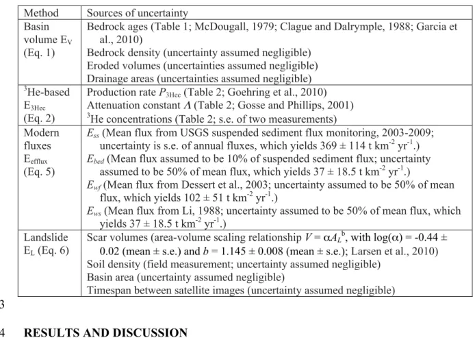
Table 4: Sources of uncertainty in erosion rate estimates
472
Method Sources of uncertainty Basin
volume EV (Eq. 1)
Bedrock ages (Table 1; McDougall, 1979; Clague and Dalrymple, 1988; Garcia et al., 2010)
Bedrock density (uncertainty assumed negligible) Eroded volumes (uncertainties assumed negligible) Drainage areas (uncertainties assumed negligible) 3He-based
E3Hec (Eq. 2)
Production rate P3Hec (Table 2; Goehring et al., 2010) Attenuation constant Λ (Table 2; Gosse and Phillips, 2001) 3He concentrations (Table 2; s.e. of two measurements) Modern
fluxes Eefflux (Eq. 5)
Ess (Mean flux from USGS suspended sediment flux monitoring, 2003-2009;
uncertainty is s.e. of annual fluxes, which yields 369 ± 114 t km-2 yr-1.)
Ebed (Mean flux assumed to be 10% of suspended sediment flux; uncertainty
assumed to be 50% of mean flux, which yields 37 ± 18.5 t km-2 yr-1.)
Ewf (Mean flux from Dessert et al., 2003; uncertainty assumed to be 50% of mean
flux, which yields 102 ± 51 t km-2 yr-1.)
Ews (Mean flux from Li, 1988; uncertainty assumed to be 50% of mean flux, which
yields 37 ± 18.5 t km-2 yr-1.) Landslide
EL (Eq. 6)
Scar volumes (area-volume scaling relationship V = αALb, with log(α) = -0.44 ± 0.02 (mean ± s.e.) and b = 1.145 ± 0.008 (mean ± s.e.); Larsen et al., 2010) Soil density (field measurement; uncertainty assumed negligible)
Basin area (uncertainty assumed negligible)
Timespan between satellite images (uncertainty assumed negligible)
473
RESULTS AND DISCUSSION
474
Spatial patterns in Myr-scale erosion rates and precipitation rates across Kaua‘i
475
Two main observations can be drawn from the pattern of Myr-scale erosion rates 476
across Kaua‘i in Figure 2. First, basin-averaged erosion rates EV vary by more than a
477
factor of 40 across the island, from as high as 335 t km-2 yr-1 to as low as 8 t km-2 yr-1, 478
with the lowest rates along the island’s west flank, the highest rates on the island’s north 479
side, and intermediate rates in the large canyons draining to the south. These Myr-scale 480
erosion rates are positively correlated with modern basin-averaged mean annual 481
precipitation rates, consistent with a positive influence of precipitation rates on erosion 482
rates (Figure 2B). Considering the absence of strong correlations between erosion rates 483
and precipitation rates in several other compilations, (e.g., Walling and Webb, 1983; von 484
Blanckenburg, 2005; Portenga and Bierman, 2011), this correlation is striking. This 485
correlation may be more apparent on Kaua‘i than elsewhere because the study basins 486
have such a large range in precipitation rates but only small variations in potentially 487
confounding factors like lithology and rock uplift rate. We stress, however, that this 488
correlation is only coarsely indicative of how rainfall rates should affect landscape 489
evolution, because estimates of EV do not reveal which erosional processes are active or
490
how sensitive each process is to rainfall rates. Indeed, the dominant processes of erosion 491
have likely changed over Kaua‘i’s lifespan, since mass fluxes on very young volcanic 492
islands tend to be dominated by subsurface chemical weathering fluxes (e.g., Rad et al., 493
2007; Schopka and Derry, 2012), while on older islands the dominant mass transport 494
processes shift to bedrock river incision, soil creep, and landsliding (e.g., Wentworth, 495
1943; Lamb et al., 2007). Ultimately, incorporating the effects of precipitation rates into 496
landscape evolution models will require quantifying how precipitation rates influence the 497
rate coefficients for specific erosion processes like bedrock river incision and hillslope 498
soil production and transport. In the final section of this paper, we consider the 499
implications of our measurements for large-scale relationships between climate, erosion, 500
and tectonics. 501
The second main observation in Figure 2 concerns the extent of basin excavation 502
fV, which we define as the ratio of the eroded rock volume to the initial rock volume that
503
was available to be eroded before erosion began – i.e., the volume of an imaginary wedge 504
defined by the basin’s present-day lateral boundaries, the initial topographic surface, and 505
sea level. This ratio can be thought of as the basin’s fractional volume loss. It is useful 506
because it is less sensitive than EV to differences among basins in the local topography
507
and thickness of the initial shield surface. That is, because EV is calculated by dividing
508
eroded volumes by basin area (Equation 1), EV may be partly dependent on the vertical
509
thickness of rock that existed between the initial topographic surface and sea level, 510
simply because more volume per unit basin area can be eroded from a thick wedge of 511
rock than from a thin wedge. Because some basins on Kaua‘i had larger initial 512
thicknesses than others, the estimates of EV in Figure 2 may partly reflect differences in
513
initial topography among basins, which may obscure the effects of climate on the 514
efficiency of basin erosion. Calculating fV, by contrast, involves normalizing eroded
515
volumes by initial basin volume, which yields a measure of basin excavation that is 516
independent of the basin’s initial topography. As Figure 2C shows, the extent of basin 517
excavation is positively correlated with modern mean annual precipitation rates above 518
precipitation rates of ~1 m/yr. Together, Figures 2B and 2C show that wetter basins have 519
higher Myr-scale erosion rates than drier basins do, and that wetter basins have lost a 520
larger fraction of their initial rock volume than drier basins have. 521
Although most basins in Figure 2 lie along a power-law trend between erosion 522
rate and mean annual precipitation, three basins draining to the Na Pali coast – Honopu, 523
Hanakapi‘ai, and Kalalau – lie above this trend. To the extent that Figure 2 implies that 524
Myr-scale erosion rates ought to scale with mean annual precipitation, the deviation of 525
these points from the trend suggests that these basins eroded anomalously quickly for 526
their climatic settings relative to the other basins on Kaua‘i. One possible explanation for 527
the high erosion rates in these three basins is rapid knickzone retreat initiated by flank 528
failure on the Na Pali coast. Some studies have interpreted the existence of large 529
knickzones in rivers draining to the Na Pali coast (and the absence of knickzones in 530
similarly sized basins draining to Kaua‘i’s west coast) as evidence for a propagating 531
wave of incision initiated by a massive flank failure on the Na Pali coast (e.g., Moore et 532
al., 1989; Seidl et al., 1994; Stock and Montgomery, 1999), similar to the suggestion that 533
a flank failure initiated a wave of incision on Hawaii’s Kohala coast (Lamb et al., 2007). 534
Although our basin-averaged erosion rate measurements cannot confirm the occurrence 535
or timing of a flank failure along the Na Pali coast, a rapidly propagating wave of river 536
incision through the channel networks would have accelerated erosion of the neighboring 537
hillslopes and generated erosional patterns that would be consistent with the erosional 538
patterns in Figure 2. 539
The basin-averaged precipitation rates in Figure 2 are inferred from rainfall 540
measurements made over the past few decades (Daly et al., 2002; PRISM Climate Group, 541
Oregon State University), an interval that is far shorter than the ~4 Myr associated with 542
the basin-averaged erosion rates. This difference in timescales is important because 543
spatial patterns in precipitation rates may have differed in the past, which would mean 544
that Kaua‘i’s topography evolved to its present state under a time-varying climate that 545
differed from the present climate. For instance, precipitation rates may have varied in 546
response to changes in regional climate, changes in the elevation of the atmospheric 547
temperature inversion, and changes in the island’s topography as it subsided and was 548
carved by rivers (e.g., Hotchkiss et al., 2000; Chadwick et al., 2003). Thus the degree to 549
which spatial patterns in modern precipitation rates are representative of spatial patterns 550
in paleoprecipitation rates depends on the degree to which the factors that controlled 551
paleoprecipitation rates – i.e., the dominant wind direction and the elevation of the 552
topography relative to that of the atmospheric inversion – were similar to those factors 553
today. 554
Unfortunately, there is only limited observational evidence to constrain past wind 555
conditions and the paleoelevation of Kaua‘i relative to the atmospheric inversion over the 556
past 5 Myr (e.g., Gavenda, 1992). The orientation of lithified sand dunes (Stearns, 1940; 557
Stearns and Macdonald 1942; 1947; Macdonald et al., 1960; Porter, 1979) and the 558
asymmetry of pyroclastic cones (Wentworth, 1926; Winchell, 1947; Porter, 1997) 559
elsewhere in the Hawaiian Islands suggest that regional winds during glacial periods were 560
dominated by northeasterly trade winds, as they are today. The existence of submarine 561
terraces encircling Kaua‘i have been interpreted as an indication that Kaua‘i has subsided 562
800-1400 m since submersion of the terraces (Mark and Moore, 1987; Flinders et al., 563
2010). There are no quantitative constraints on the atmospheric inversion layer altitude 564
over time, but palynological evidence on Oahu suggests that low- to mid-elevation 565
windward sites received more precipitation during glacial periods than at present, which 566
has been interpreted as an indication that the inversion layer was lower during glacial 567
periods than at present (Hotchkiss and Juvik, 1999). These observations suggest that a 568
portion of Kaua‘i may have spent some time above the atmospheric temperature 569
inversion over the past 4-5 Myr, given that (1) the modern elevation of the atmospheric 570
temperature inversion fluctuates between ~1800 m and ~2700 m (Ramage and Schroeder, 571
1999); (2) Kaua‘i’s highest point is currently at an elevation of 1593 m; (3) Kaua‘i was 572
likely 800-1400 m higher before subsidence; and (4) the atmospheric inversion was likely 573
at lower altitudes during glacial periods. If this is true, then the portion of the island 574
above the temperature inversion may have been drier than sites below the inversion, and 575
the spatial pattern of precipitation rates across Kaua‘i may have differed from that at 576
present. 577
Hotchkiss et al. (2000) attempted to account for changes in topography, regional 578
climate, and the atmospheric inversion altitude in a model of soil development at one site 579
on Kaua‘i’s Kokee ridge, and concluded that the mean annual precipitation rate at that 580
site over the past 4.1 Myr was roughly 87% of the present-day mean annual precipitation 581
rate, which suggests that modern rainfall rates may be similar to those over the past 4.1 582
Myr. To the extent that their model is accurate and Kokee Ridge is representative of 583
Kaua‘i as a whole, this model result suggests that modern precipitation rates may be a 584
reasonable proxy for the paleoprecipitation rates that influenced Kaua‘i’s topographic 585
evolution. 586
Irrespective of how spatial patterns in precipitation rates across Kaua‘i have 587
evolved over the past 4-5 Myr, there remains a positive correlation between the Myr-588
scale basin-averaged erosion rates in Figure 2B and modern basin-averaged precipitation 589
rates. Such a strong correlation would be surprising if spatial patterns in 590
paleoprecipitation rates were very different from those at present. If that were the case, 591
the correlation in Figure 2B would imply that erosion rates were controlled by factors 592
other than mean annual precipitation that fortuitously covaried with modern mean annual 593
precipitation. There are, however, no obvious non-climatic factors (e.g., lithology, rock 594
uplift rates) that covary with mean annual precipitation across Kaua‘i and which might 595
strongly affect erosion rates. We acknowledge that it is possible that other moments of 596
precipitation, such as storminess, might also covary with mean annual precipitation and 597
might influence long-term erosion rates (e.g., DiBiase and Whipple, 2011), but the 598
simplest explanation for the correlation in Figure 2B is a dependence of erosion rates on 599
mean annual precipitation. 600
601
Modern, million-year, and millennial erosion rates in the Hanalei basin
602
Annual suspended sediment discharges at the Hanalei River monitoring station 603
(USGS gauge 16103000) between 2003 and 2009 range from 153 t km-2 yr-1 to 690 t km-2 604
yr-1, with a mean and standard error of Ess = 369 ± 114 t km-2 yr-1. Dessert et al. (2003)
605
reported 1971-1976 USGS measurements of runoff (3.6 m/yr) and total dissolved solids 606
(28.3 mg/l) in the Hanalei River, which imply a fluvial solute flux of 102 t km-2 yr-1. In 607
the absence of measurements on atmospheric solute inputs or changes in intra-basin 608
solute storage over the same time period, we take this to be representative of the fluvial 609
chemical erosion rate Ewf. Li (1988) estimated that groundwater discharge to the ocean is
610
responsible for an additional Ews = 37 t km-2 yr-1 of subsurface solute losses across
611
Kaua‘i, calculated as the product of the island-average groundwater recharge rate and the 612
mean chemical composition of groundwater. For the purposes of estimating the total 613
mass flux in the Hanalei basin, we tentatively assume that fluvial solute fluxes in the 614
Hanalei basin in 2003-2009 were comparable to those in 1971-1976, and that subsurface 615
chemical erosion rates in the Hanalei basin match the island-wide subsurface chemical 616
erosion rate in Li (1988). This is an approximation. Fluvial solute fluxes between 2003 617
and 2009 might have differed from those between 1971 and 1976, and subsurface solute 618
fluxes from the Hanalei basin (which is wetter than most basins on Kaua‘i) might differ 619
from island-average subsurface solute fluxes. Neither Dessert et al. (2003) nor Li (1988) 620
reported uncertainties on the reported solute fluxes, despite a number of potential sources 621
of error in the determination of fluvial and subsurface solute fluxes (e.g., uncertainties in 622
evapotranspiration rates, atmospheric solute deposition rates, and short-term changes in 623
solute storage in biota or the subsurface). To be conservative, we apply 50% 624
uncertainties to both the fluvial and subsurface solute flux estimates, and calculate the 625
Hanalei basin’s total chemical erosion rate as Ewf + Ews = (102 ± 51 t km-2 yr-1) + (37 ±
626
18.5 t km-2 yr-1) = 139 ± 54 t km-2 yr-1. 627
These estimates can be compared with Kaua‘i-wide estimates of surface and
628
groundwater fluxes of dissolved silica and total alkalinity (Schopka and Derry, 2012).
629
We convert Schopka and Derry’s reported fluxes from mol/yr to t km-2 yr-1 using the area
630
of Kaua‘i (1437 km2), a molar mass of 60.08 g/mol for silica, and an average molar mass
631
of 63.1 g/mol for total alkalinity (i.e., the average molar mass of the oxides of the major
632
cations that balance the charge in the total alkalinity (Na2O, K2O, CaO, and MgO)). With
633
this conversion, we calculate that Schopka and Derry’s Kaua‘i-wide estimates of surface
634
solute fluxes (68 ± 20 t km-2 yr-1) and groundwater solute fluxes (33 ± 9 t km-2 yr-1) agree
635
with our estimates within uncertainty, which suggests that our estimates of solute fluxes
636
in the Hanalei basin are of reasonable magnitude. In the absence of empirical constraints
637
on bedload fluxes in the Hanalei basin or elsewhere on Kaua‘i, we tentatively take 638
bedload fluxes at the Hanalei gauging station to be 10 ± 5% of the physical sediment 639
flux, for a physical sediment flux of Ess + Ebed = (369 ± 114 t km-2 yr-1) + (0.1 ±
640
0.05)(369 ± 114 t km-2 yr-1) = 406 ± 116 t km-2 yr-1. Combining these estimates yields a 641
total mass flux of Eefflux = (406 ± 116 t km-2 yr-1) + (139 ± 54 t km-2 yr-1) = 545 ± 128 t
642
km-2 yr-1 from the Hanalei basin. 643
Because suspended sediment fluxes were monitored in the Hanalei basin only 644
from 2003 to 2009, it is not possible to directly quantify how representative sediment 645
fluxes during this period were relative to those during the previous decades. However, 646
water discharges measured in the Hanalei River during 58 years of monitoring up to the 647
present suggest that the basin did not experience unusually intense storms during the 648
2003-2009 period (USGS National Water Information System). The Hanalei River’s 649
largest peak discharge during the 2003-2009 monitoring period occurred in February 650
2006, and it had an intensity that is exceeded by 19 floods during the 58 years on record, 651
including two floods that occurred after suspended sediment monitoring ended in 2009. 652
Thus, the Hanalei River’s hydrologic monitoring record suggests that the largest floods 653
between 2003 and 2009 were not unusually large relative to floods before or since, which 654
in turn suggests that our estimates of Hanalei mass fluxes during this interval are unlikely 655
to be skewed high by the 2006 storm event. 656
These calculations suggest that modern mass fluxes from the Hanalei basin (545 ± 657
128 t km-2 yr-1) are at least 1.8 ± 0.5 and at most 3.1 ± 0.8 times faster than mass fluxes 658
from the Hanalei basin averaged over the past several million years (which have 659
minimum and maximum bounds of 175 t km-2 yr-1 and 309 t km-2 yr-1, respectively; Table 660
1). By comparison, minimum bounds on kyr-scale erosion rates E3Hec based on 3He
661
concentrations in detrital olivine range from >126 to >390 t km-2 yr-1 (Table 2). As 662
described in the Methods section, these are minimum bounds on erosion rates because 663
they rest on the assumption that all the measured 3He is cosmogenic. These erosion rates
may be considered averages over characteristic timescales Λ/ E3Hec of <12.7 kyr to <4.1
665
kyr, respectively. 666
These estimates of E3Hec differ among tributary basins by a factor of three, which
667
we suggest is not large; such differences in cosmogenically-inferred erosion rates are 668
common among small tributary basins (e.g., Ferrier et al., 2005). The basin-to-basin 669
differences in E3Hec may reflect inter-basin differences in erosion rates or radiogenic 4He
670
concentrations, or they may reflect intra-basin variability in 3He concentrations and the 671
relatively small number (n ~ 100) of olivine grains in the samples in which 3He 672
concentrations were measured (e.g., Gayer et al., 2008). These minimum bounds on 673
millennial-scale erosion rates bracket the only other basin-averaged erosion rates inferred 674
from detrital 3Hec on Kaua‘i (168 t km-2 yr-1 in the Waimea River; Gayer et al., 2008),
675
and are similar to the estimates of Myr-scale erosion rates in the Hanalei basin and the 676
Waimea basin (Table 1). The measured 3He concentrations offer no upper bounds on 677
kyr-scale erosion rates, but the minimum bounds on E3Hec are consistent with the
678
possibility that erosion rates in the Hanalei basin over the past few thousand years were 679
comparable to erosion rates in the Waimea basin over the past few thousand years, as 680
well as to erosion rates in the Hanalei basin over the past few million years. 681
The most relevant 3He-based erosion rate to compare to modern stream sediment 682
fluxes is the rate of >238 t km-2 yr-1 at site HAN017 (Figure 3), because this sample was 683
collected at the site of the USGS Hanalei River gauging station and therefore averages 684
over the same drainage area (47.9 km2 of the Hanalei basin’s total drainage area of 60.0 685
km2) as the modern suspended sediment fluxes do. What fraction of the modern mass 686
flux should the 3He-based erosion rates be compared to? Erosion rates inferred from 3Hec