Control and estimation strategies for autonomous MAV landing on a moving platform in turbulent wind conditions

Control and Estimation Strategies for Autonomous

MAV Landing on a Moving Platform in Turbulent

Wind Conditions

by

Aleix París i Bordas

Submitted to the Department of Aeronautics and Astronautics

in partial fulfillment of the requirements for the degree of

Master of Science in Aeronautics and Astronautics

at the

MASSACHUSETTS INSTITUTE OF TECHNOLOGY

June 2020

c

○ Massachusetts Institute of Technology 2020. All rights reserved.

Author . . . .

Department of Aeronautics and Astronautics

May 19, 2020

Certified by . . . .

Jonathan P. How

Richard C. Maclaurin Professor of Aeronautics and Astronautics

Thesis Supervisor

Accepted by . . . .

Sertac Karaman

Associate Professor of Aeronautics and Astronautics

Chair, Graduate Program Committee

Control and Estimation Strategies for Autonomous MAV

Landing on a Moving Platform in Turbulent Wind Conditions

by

Aleix París i Bordas

Submitted to the Department of Aeronautics and Astronautics on May 19, 2020, in partial fulfillment of the

requirements for the degree of

Master of Science in Aeronautics and Astronautics

Abstract

Micro aerial vehicles (MAVs) are increasing in popularity both for recreational and commercial purposes. In particular, autonomous MAVs are promising in the field of drone delivery due to their scalability, deployability, and low cost compared to tradi-tional ground delivery. Hybrid systems, which combine MAVs taking off and landing from/to trucks and the ground vehicles themselves to increase package delivery ef-ficiency, present even more advantages. Nevertheless, these systems require reliable control strategies that account for the challenging environment present in the vicinity of moving ground vehicles, as well as techniques to estimate these conditions.

This thesis presents a novel planning and control strategy that allows a fast, au-tonomous landing of a micro aerial vehicle (MAV) on a moving ground vehicle, which will be required for truck-drone delivery systems. The turbulent wind conditions near the landing platform are measured online using small, inexpensive whisker-like sen-sors. The measurements from these sensors are then used by an unscented Kalman filter to estimate the wind speed acting on the MAV, which is then compensated for by a boundary layer sliding controller. The experiments performed validate the robustness of the approach, which allows fast, dynamic landings of a MAV in moving ground vehicles in challenging environments without the need for hovering above the landing platform first.

Thesis Supervisor: Jonathan P. How

Acknowledgments

First, I would like to thank my advisor Jonathan How for his help and guidance. His insights have been of great value for the papers I have published during my Master’s, and for this thesis. Thank you as well for giving me the opportunity to study my M.S. at MIT, and thanks to Ford Motor Company for providing me funding to do so. I am very grateful to my colleagues at the Aerospace Controls Laboratory. Jesus, Samir, Dong Ki, Jeremy, Andrea, Lena, Parker, Michael, Stewart, Rose, Sebastian, Brett, Kaveh... Thank you all for your feedback, fruitful discussions, and for being a source of inspiration. Bryt, thanks for your help handling my frequent purchase orders.

I would also like to thank my family away from home. Toni, Bruno, Antonella, Íñigo, Juanjo, Marc, and the MIT Cheerleading team: thanks for making sure I spent time outside the lab too.

Of course, I also want to acknowledge my partner Ruiya, for being very under-standing and supportive during stressful times. The motivation and energy you always give me are invaluable.

Last, and definitely not least, my deepest gratitude goes to my family. Jordi, Gerard, this would not have been possible without you. You are a source of strength and support, and I know I can always count on you. Thanks, a lot.

Contents

1 Introduction 13

1.1 Motivation . . . 13

1.2 Literature Review . . . 14

1.3 Thesis Aims and Outline . . . 16

2 Dynamic Landing with Wind Measured a Priori 19 2.1 Introduction . . . 19

2.1.1 Contributions . . . 20

2.2 System Overview . . . 21

2.2.1 Finite State Machine . . . 22

2.2.2 Trajectory Planning: Model Predictive Control . . . 22

2.2.3 Ancillary Controller: Boundary Layer Sliding Controller . . . 24

2.2.4 Landing Platform Estimation: Extended Kalman Filter . . . . 26

2.2.5 Visual Detection: AprilTag Visual Fiducial System . . . 27

2.3 Experimental Results . . . 28

2.3.1 Hardware . . . 28

2.3.2 Static Platform Experiments . . . 29

2.3.3 Moving Platform Experiments . . . 32

3 Wind Estimation 35 3.1 Introduction . . . 35

3.2 Sensor Design . . . 37

3.2.2 Sensor Design and Considerations . . . 38

3.2.3 Sensor Measurements . . . 39

3.3 Model-based Approach . . . 40

3.3.1 MAV Dynamic Model . . . 41

3.3.2 Airflow Sensor Model . . . 42

3.3.3 Model-based Estimation Scheme . . . 44

3.4 Deep Learning-based Approach . . . 46

3.4.1 Output and Inputs . . . 47

3.4.2 Network Architecture . . . 47

3.4.3 Interface with the Model-based Approach . . . 48

3.5 Experimental Evaluation . . . 48

3.5.1 System Identification . . . 48

3.5.2 Implementation Details . . . 50

3.5.3 Relative Airflow Estimation . . . 52

3.5.4 Wind Gust Estimation . . . 52

3.5.5 Simultaneous Estimation of Drag and Interaction Forces . . . 54

4 Dynamic Landing with Wind Measured in Real Time 57 4.1 Introduction . . . 57

4.2 Simulation Environment . . . 57

4.2.1 MAV Simulation . . . 58

4.2.2 Airspeed Sensor Simulation . . . 58

4.2.3 Wind Simulation . . . 59

4.2.4 UGV Simulation and Visualization . . . 60

4.3 Results . . . 60

5 Conclusion 65 5.1 Thesis Summary . . . 65

5.2 Limitations and Future Work . . . 66

List of Figures

2-1 Dynamic landing maneuver on a moving platform . . . 20

2-2 Dynamic landing trajectory . . . 20

2-3 Diagram of the system’s architecture . . . 21

2-4 Finite state machine . . . 22

2-5 Quadrotor vehicle used for the dynamic landing experiments . . . 28

2-6 Leaf blower array and static platform . . . 30

2-7 Mean wind speed and standard deviation from the leaf blowers . . . . 30

2-8 Static platform, standard BLSC . . . 31

2-9 Static platform, disturbance-aware BLSC . . . 31

2-10 Landing platform with vertical tag bundle . . . 33

2-11 Ground vehicle leaf blowers assembly . . . 33

2-12 Landing platform on dolly towed by UGV . . . 34

2-13 Moving platform, disturbance-aware BLSC . . . 34

3-1 MAV with four bio-inspired sensors . . . 36

3-2 Bend Labs sensor . . . 37

3-3 Bend Labs sensors on hexarotor . . . 38

3-4 Airflow sensor . . . 40

3-5 Model-based approach diagram . . . 42

3-6 Learning-based approach diagram . . . 46

3-7 Sensor deflection angle vs wind speed . . . 49

3-8 Model- and learning-based relative velocity comparison . . . 51

3-10 Simultaneous estimation of drag and interaction force – setup . . . . 55 3-11 Simultaneous estimation of drag and interaction force – plots . . . 55 4-1 Gazebo environment . . . 60 4-2 Moving platform, standard BLSC . . . 62 4-3 Moving platform, disturbance-aware BLSC with online wind estimation 63

List of Tables

3.1 RMS between LSTM and UKF . . . 54 4.1 Wind parameters . . . 61

Chapter 1

Introduction

1.1

Motivation

Autonomous unmanned aerial vehicles (UAVs) are becoming more popular in industry because of their flexibility and fast deployment. UAVs have demonstrated their utility in applications such as aerial photography for topology and agriculture [1–4], search and rescue operations [5, 6], and mapping [7–9], both alone and in drone formations [10, 11]. The large recent growth in online shopping has also attracted interest in reducing package shipment time and costs, and UAVs provide an efficient alternative to delivery trucks [12, 13]. However, their payload and flight time is limited, so several researchers have investigated using a truck-drone delivery system [14, 15]. The UAVs in current truck-drone delivery methods can only take off and land when the truck is stopped visiting a customer node, which has substantial synchronization costs. Thus, autonomous landing on a moving truck offers some further efficiencies [16].

Additionally, the deployment of micro aerial vehicles (MAVs) in uncertain and constantly changing atmospheric conditions [17–19] requires the ability to estimate and adapt to disturbances such as the aerodynamic drag force applied by wind gusts. Simultaneously, as many new interaction-based missions [20–22] arise, so increases the need to better differentiate between forces caused by aerodynamic disturbances and other sources of interaction [23–26]. Differentiating between aerodynamic drag force and interaction force can be extremely important for safety reasons. For example, the

controller of a robot should react differently depending on whether a large disturbance is caused by a wind gust, or by a human trying to interact with the machine [27].

Distinguishing between drag and interaction disturbances can be challenging, as they both apply forces to the center of mass (CoM) of the multirotor that cannot be easily differentiated by examining the inertial information commonly available from the robot’s onboard IMU or odometry estimator. Successful approaches for this task include a model-based method that measures the change in thrust-to-power ratio of the propellers caused by wind [28] and an approach which monitors the frequency component of the total disturbance (estimated via inertial information) to distinguish between the two possible sources of force [29].

This thesis presents a strategy for simultaneously estimating the interaction force and the aerodynamic drag disturbances using novel bio-inspired, whisker-like sensors that measure the airflow around a multirotor, as shown in Fig. 3-1. The estimated wind speed is then used by an ancillary controller that is able to reject the disturbances acting on the MAV and allows a fast landing maneuver on a moving platform.

1.2

Literature Review

Autonomous UAV landing has been investigated by several researchers. Ref. [30] landed a drone on a static kayak in a reservoir with mild wind and water ripple conditions, but the image processing was done off-board and the landing time was close to 1 min. Ref. [31] developed a system capable of landing a UAV on a moving platform with PID control, an EKF estimator, and an AprilTag visual fiducial bundle. However, the computation was also done off-board, and there was no relative wind present: the platform’s speed was just 0.18m/s and the tests were done indoors. Ref. [32] demonstrated a quadrotor landing on a moving platform using only onboard sensing and computation, but the environment was not turbulent due to the tests being indoors and the platform was moving relatively slowly at 1.2m/s. Furthermore, besides two cameras, a distance sensor was required to estimate the UAV-platform relative pose. Ref. [33] demonstrated an autonomous landing of a quadrotor on a car

moving at 14m/s by detecting an AprilTag on its roof. A proportional navigation-based guidance law was used for the approach phase, and a PID controller for the landing phase, with no disturbance rejection considerations. The landing maneuver consisted of acquiring the tag while hovering, and the descent was initiated once the quadrotor stabilized over it. Additionally, the quadrotor used was large and had a broad sensor suite, including a downward-facing camera, a three-axis gimballed camera to track the target, and an inertial navigation system. Furthermore, besides the ground vehicle’s GPS coordinates, the quadrotor also used the ground vehicle’s IMU data to improve its estimation of the landing platform’s state. Ref. [34] also demonstrated an outdoors landing, but the landing platform’s speed was only 0.5m/s and the landing maneuver took 12–20 s to complete. Moreover, the ground vehicle’s wheel encoders data was used to estimate its state. Ref. [35] used model predictive control (MPC) to land a quadrotor on a moving ship. Both the UAV and the ship collaborated to reach their goal. The waves were modeled as sinusoidal, but the wind disturbances considered were not turbulent – this approach only compensated the effects caused by a steady-state wind. Furthermore, the vehicle needed to hover above the platform for at least 5 s, and the ship was simulated. A simulated boat landing was also carried out in [36], where the platform’s state was estimated fusing GPS and visual measurements. This work incorporated a velocity feed-forward term to the controller to catch the platform, but its only consideration of external wind was an offset of the hovering position to ensure the target was inside the field of view of the downwards-facing camera, and the landing maneuver lasted 24 s. Ref. [37] developed an adaptive controller to track a ground vehicle with only relative position data from ArUco tags, and tested it in outdoor experiments at 5.6 m/s. But this approach only considered disturbances due to ground effect, and the landing maneuver needed 20 s for tracking and 10 s for descent.

In summary, most current approaches for MAV landing on moving platforms in-volve hovering above the platform for a period of time to visually acquire it, which is then followed by a relatively slow descent. In contrast, the approach presented in this thesis investigates a direct trajectory to the landing platform, which has the

pos-sible advantages of providing faster landings and enabling several UAVs to approach the platform at the same time from different directions (improving the utilization of this limited resource). Additionally, most of current approaches do not make special considerations to reject the turbulent wind present near the target vehicle, and thus safety in challenging conditions cannot be guaranteed.

In regard to distinguishing between interaction and aerodynamic disturbance, most of the current approaches focus on the estimation of one or the other disturbance only.

Aerodynamic disturbances: Accurate wind or airflow sensing is at the heart of the techniques employed for aerodynamic disturbance estimation. A common strategy is based on directly measuring the airflow surrounding the robot via sensors, such as pressure sensors [38], ultrasonic sensors [39], or whisker-like sensors [40]. Other strategies estimate the airflow via its inertial effects on the robot, for example using model-based approaches [41, 42], learning-based approaches [43, 44], or hybrid (model-based and learning-(model-based) solutions [45].

Generic wrench-like disturbances: Multiple related works focus instead on es-timating wrench disturbances, without explicitly differentiating for the effects of the drag force due to wind: [22–24, 46] propose a model-based approach which utilizes an unscented Kalman filter (UKF) for wrench estimation, while [47] proposes a factor graph-based estimation scheme.

1.3

Thesis Aims and Outline

This thesis presents a system capable of landing a MAV on a moving platform, even in the presence of turbulent wind. First, a boundary layer sliding controller (BLSC) that takes into account these conditions is presented, as well as a planner with changing objectives that allows a fast maneuver, and a vision-based extended Kalman filter (EKF) to estimate the moving platform’s state. The UAV’s state estimator used a motion capture system, but the important information in the demonstrated maneuver

(the relative position of the UAV and the moving platform) is estimated onboard by the quadrotor using a vision system. Then, an unscented Kalman filter (UKF) is presented, which uses bio-inspired sensors to estimate online the wind speed acting on the vehicle. Both a model- and a learning-based strategy are introduced and compared.

The previous section identified a research gap in the fields of control and estimation for MAVs in windy conditions. Therefore, this thesis has three main goals:

∙ To develop a planning and control strategy that allows an UAV to fly in chal-lenging conditions and land rapidly on a moving platform

∙ To design a reliable wind estimation technique

∙ To validate, both in simulation and in hardware experiments, the robustness of the approach

The remainder of this thesis is organized as follows:

Chapter 2 introduces the control strategy used in this work, a boundary layer sliding controller, as well as a planning strategy that allows a MAV to land on a moving platform in turbulent wind conditions from which the mean and standard deviation have been measured beforehand.

Chapter 3 presents model- and deep learning-based approaches to estimate the wind acting on a MAV using bio-inspired, whisker-like sensors.

The strategies presented in Chapter 2 and Chapter 3 are used simultaneously in Chapter 4 to demonstrate a MAV landing on a moving platform in turbulent wind conditions measured in real time. The wind speed estimation obtained with a UKF is sent to the ancillary boundary layer sliding controller to reject the disturbances acting on the vehicle.

Finally, Chapter 5 concludes this thesis by summarizing it, presenting its contri-butions and limitations, and proposing future work.

Chapter 2

Dynamic Landing with Wind

Measured a Priori

This chapter is based on [26]. This paper was accepted to the International Conference on Robotics and Automation (ICRA) 2020, taking place virtually from May 31 to August 31.

2.1

Introduction

Autonomous landing on a moving platform presents unique challenges for multirotor vehicles, including the need to accurately localize the platform, fast trajectory plan-ning, and precise/robust control. Previous works studied this problem but most lack explicit consideration of the wind disturbance, which typically leads to slow descents onto the platform. This chapter presents a fully autonomous vision-based system that addresses these limitations by tightly coupling the localization, planning, and control, thereby enabling fast and accurate landing on a moving platform. The plat-form’s position, orientation, and velocity are estimated by an extended Kalman filter using simulated GPS measurements when the quadrotor-platform distance is large, and by a visual fiducial system when the platform is nearby. The landing trajectory is computed online using receding horizon control and is followed by a boundary layer sliding controller that provides tracking performance guarantees in the presence of

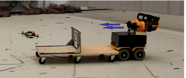
un-Figure 2-1. Dynamic landing maneuver on a moving platform in a wind environment generated by two leaf blowers.

known, but bounded, disturbances. To improve the performance, the characteristics of the turbulent conditions are accounted for in the controller. The landing trajectory is fast, direct, and does not require hovering over the platform, as is typical of most state-of-the-art approaches (see Fig. 2-2). The experiments presented validate the robustness of the approach.

Figure 2-2. Dynamic landing trajectory (green) compared with traditional landing maneuvers on moving platforms (red). An AprilTag bundle composed of 2 tags is placed in the ground vehicle to allow accurate detection by the MAV with its onboard camera, as explained in Section 2.2.5. The proposed approach is fast and efficient, and will be crucial for truck-drone delivery systems.

2.1.1

Contributions

This chapter demonstrates a vision-based system capable of dynamic landing (i.e., the multirotor does not need to hover above the vehicle before descending) which also

Boundary Layer Sliding Controller (BLSC) Model Predictive Control (MPC) 𝑢 Quadrotor Finite State Machine (FSM) Quaternion-based attitude controller Motion capture system Onboard

camera AprilTags visualFiducial system Extended Kalman Filter (EKF)

Nonlinear observer IMU Predicted 𝑥 White noise generator 𝑥∗_{, 𝑢}∗ Throttle commands 𝑥 𝑧 𝑥 Wind estimator Wind speed

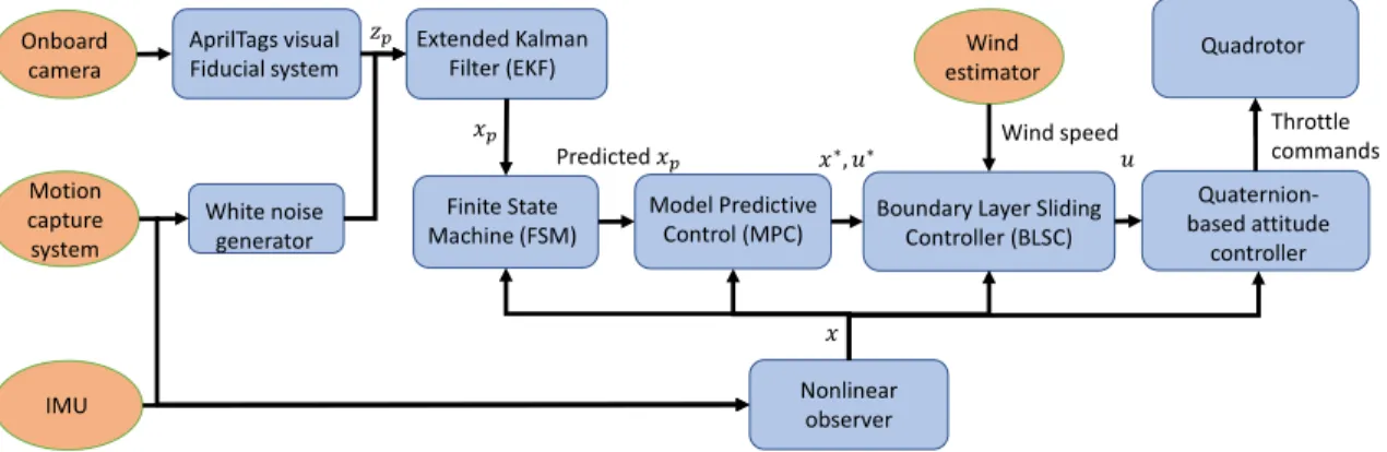
Figure 2-3. Diagram of the system’s architecture. Orange circles represent the inputs to the system, and blue squares represent each component. The arrow’s label indicates the information that is sent.

accounts for the turbulent conditions that would be present near a rapidly-moving ground vehicle. The resulting framework allows thus a maneuver that will be crucial for efficient truck-drone delivery systems. The contributions of this chapter are:

∙ Demonstration of a boundary layer sliding controller to incorporate and com-pensate for turbulence based on a model of the conditions near the landing platform.

∙ An algorithm for computing fast, vision-based dynamic landing maneuvers, is demonstrated in hardware experiments that include challenging turbulent wind conditions.

2.2

System Overview

This chapter addresses the current limitations of landing on a moving platform by: 1. Using optimization-based trajectory generation to enable dynamic landing; and 2. Using robust control to explicitly compensate for turbulent wind conditions The system that achieves this is comprised of several components, described in this section and shown in Fig. 2-3.

Stand By Search Landing End Start command Platform found UAV-UGV distance and_{relative velocity small}

Platform lost

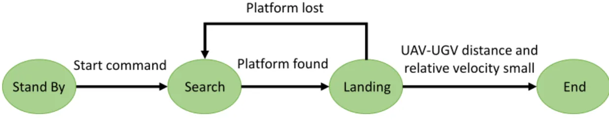
Figure 2-4. Diagram of the finite state machine.

2.2.1

Finite State Machine

The quadrotor’s behavior is determined by a finite state machine (FSM) shown in Fig. 2-4 and comprised of four states:

1. Stand By: This is the initial state of the quadrotor, which consists of taking off and hovering at a predefined altitude above the starting point. The FSM then transitions to Search mode.

2. Search: The quadrotor uses simulated GPS coordinates of the unmanned ground vehicle (UGV) —as explained in Section 2.2.4— to predict a rendezvous location and flies there. When the front-facing camera detects the landing platform as described in Section 2.2.5, the state automatically switches to Landing.

3. Landing: In this mode, the quadrotor approaches the target following a direct trajectory towards it. When the distance and relative velocity UAV-UGV are below threshold values, the quadrotor switches to the End mode. If the last detection happened more than 0.8s ago, the mode returns to Search.

4. End : motors are stopped, maneuver is finished.

2.2.2

Trajectory Planning: Model Predictive Control

The planner solves a convex optimization problem with changing objectives depending on the state of the FSM. In Search mode, the UAV-UGV rendezvous point is predicted by assuming a constant linear velocity and yaw rate for the UGV, and a constant velocity for the UAV. This position is then offset by a small distance backwards in

the direction of the UGV to ensure target detection by the front-facing camera, and is used by the planner as the final position of the trajectory, while the final velocity is the UGV’s. The time taken to reach the UGV is minimized, to reduce delivery turnarounds. In Landing mode, the planner initially minimizes the jerk to obtain a trajectory which ensures adequate tag acquisition. As the UAV approaches the target, the effect of disturbances increases so the planner minimizes the time spent in the turbulent area. The final position of the planned trajectory is the vertical tag’s position (offset a few cm backwards) and predicted ahead (by an amount that depends on the computation time) assuming constant linear/angular velocities. The final velocity of the trajectory is set to match the UGV’s.

The minimum jerk approach produces smooth trajectories and has a long heritage for planning quadrotor paths [32, 48, 49]. The trajectory is re-planned using an MPC approach every time a new estimate of the platform’s position is obtained. CVXGEN [50] generated the code to solve the following convex optimization problem

min 𝑥,¯𝑢 𝐽 = 𝑁 ∑︁ 𝑡=0 ℓ (¯𝑢, 𝑑) [𝑡] subject to 𝑥[𝑡 + 1] = 𝐴𝑥[𝑡] + 𝐵 ¯𝑢[𝑡] |𝑎[𝑡]|∞ ≤ 𝑎max |¯𝑢[𝑡]|∞ ≤ 𝑗max 𝑥[0] = 𝑥0, 𝑥[𝑁 ] = 𝑥𝑓 for 𝑡 = 0 . . . 𝑁 (2.1)

where 𝑁 is the timestep when the quadrotor has to reach the final state 𝑥𝑓, ℓ is a

quadratic cost function, ¯𝑢 is the open-loop control input (the jerk of the trajectory), 𝑑 is the UAV-tag distance, 𝑥 is the position, velocity, and acceleration of the UAV, 𝐴 and 𝐵 are, respectively, the state and input matrices for a triple integrator, and 𝑎 is the subvector of 𝑥 representing the acceleration. Note that it is possible to plan using this linear model for a nonlinear system because the nonlinear dynamics of the quadrotor are canceled by the ancillary controller, as explained next.

2.2.3

Ancillary Controller: Boundary Layer Sliding Controller

While MPC has been used extensively in industry [51], the control of systems with nonlinear dynamics requires expensive optimization. Sliding control [52] has proven to be effective in quadrotors [53, 54]. This control strategy guarantees bounds on the tracking error and has been combined with MPC [55, 56]. In this thesis’ approach, a disturbance-aware boundary layer sliding controller (BLSC) is derived, which is a nonlinear ancillary controller that models the disturbances found near the landing platform and leverages sliding control techniques.

In quadrotors, the attitude dynamics are much faster than the position dynamics, and thus control of both can be decoupled [57]: the output of a controller is the setpoint for the other. The position and velocity controller is derived in this section to account for the turbulent wind present near the landing platform, and the attitude control is performed by a quaternion-based controller [58].

The following derives the BLSC. Define the manifold 𝑆(𝑡) by 𝑠 = ˙˜𝑥 + 𝜆˜𝑥 = 0, where ˜𝑥 = 𝑥 − 𝑥𝑑 and 𝜆 > 0. The objective of sliding control is to maintain 𝑠 = 0

at all times. If the control action’s frequency is high enough, zero tracking error is guaranteed [52]. This high control action is impractical in many applications because of actuator limits and the excitation of unmodelled dynamics. An approach taken in [53, 56] is BLSC, where the control discontinuity is smoothed in a thin boundary layer of thickness Φ:

B := {𝑠 : |𝑠| ≤ Φ} (2.2)

Consider a system whose dynamics can be expressed as

¨

𝑥 = 𝑓 (𝑥) + 𝑏 (𝑥) 𝑢 + 𝑑 (2.3)

where 𝑑 is the disturbance. Then, the BLSC strategy is

𝑢 = ˆ𝑏−1[︁𝑥¨𝑑− 𝜆 ˙˜𝑥 − ˆ𝑓 (𝑥) − 𝐾 sat

(︁𝑠 Φ

)︁]︁

(2.4)

and 𝐾 is determined by the uncertainty in the dynamics and the disturbance of the system. As noted before, in (2.1) it is possible to plan using linear MPC because of the cancellation of 𝑓 in (2.3) and (2.4).

The leaf blowers generate turbulence as shown in Fig. 2-1 and Fig. 2-6. The turbulent wind parameters are the mean 𝑣𝑤 and standard deviation 𝜎 of the speed.

Define 𝑉 = 𝑣 + 𝑣𝑤where 𝑣 is the quadrotor’s speed. Then, 𝑉 is the total wind speed

relative to the UAV and ˆ𝑓 is ˆ𝑓 = ˆ𝑐 ‖𝑉 ‖ 𝑉, where ˆ𝑐 is the estimated drag coefficient of the quadrotor.

The quadrotor plans a trajectory to approach the UGV in the direction it is facing to match its speed, and thus is never outside the wind field generated by the leaf blowers during the landing maneuver. Therefore, it is reasonable to assume that this wind field is constant in the directions perpendicular to where the leaf blowers point to. The true acceleration caused by drag is

𝑓 = 𝑐 ‖𝑉 ± 2𝜎𝑢𝑤‖ (𝑉 ± 2𝜎𝑢𝑤) (2.5)

where 𝑢𝑤 is a unit vector in the direction of the wind.

The variation of 𝑏 is very small for a UAV with constant weight. Therefore, 𝛽 = (𝑏𝑚𝑎𝑥/𝑏𝑚𝑖𝑛) is approximately 1, where 𝑏𝑚𝑎𝑥 and 𝑏𝑚𝑖𝑛 are the maximum and

minimum control gains respectively (or throttle gains in the context of quadrotors). Thus, 𝐾 is simplified as [52] 𝐾 = ¯𝐹 + 𝜂, where 𝜂 > 0 is a constant in the sliding condition 1 2 𝑑 𝑑𝑡𝑠 2 _{≤ −𝜂|𝑠|. (2.6)}

The larger the 𝜂, the faster the system will reach the sliding surface. Nevertheless, 𝐾 should only be as large as the disturbance magnitude requires to avoid a high-frequency control signal. ¯𝐹 is

𝐹 =|𝑓 − ˆ𝑓 | ≤ ¯𝐹 ¯

𝐹 =| (ˆ𝑐 + ˜𝑐) ‖𝑉 ± 2𝜎𝑢𝑤‖ (𝑉 ± 2𝜎𝑢𝑤) − ˆ𝑐 ‖𝑉 ‖ 𝑉 |

where ˜𝑐 > 0 is a bound on the absolute value of the drag coefficient error |𝑐 − ˆ𝑐|. By taking the sign that makes this coefficient larger, 𝐾 is defined. In this application, the quadrotor moves towards the generated wind and therefore this occurs when the 2𝜎 is increasing the magnitude of 𝑣𝑤.

2.2.4

Landing Platform Estimation: Extended Kalman Filter

To estimate the state of the moving platform, an extended Kalman filter (EKF) is used. This filtering algorithm minimizes the mean of the squared error and has demon-strated its efficacy in robot localization [59–61]. The state vector of the platform is 𝑥𝑝= [𝑝𝑥, 𝑝𝑦, 𝑣𝑝, 𝜃, ˙𝜃]⊤, where 𝑝𝑥, 𝑝𝑦 are the 2D coordinates, 𝑣𝑝 is the magnitude of the

velocity, 𝜃 is the orientation angle with respect to the 𝑥-axis, and ˙𝜃 is the angular ve-locity. Since real-world roads are mostly horizontal and in particular the experiments in this thesis were carried on completely flat surfaces, the velocity in the 𝑧-direction is not estimated. The moving platform is modeled as a unicycle with dynamics

˙

𝑥𝑝(𝑡) = 𝑓𝑝(𝑥𝑝(𝑡)) + 𝑤(𝑡), (2.8)

where 𝑤(𝑡) is the process noise, assumed to be a white Gaussian noise. A constant linear and angular velocity are considered, and the UGV dynamics are

˙

𝑝𝑥 = 𝑣𝑝cos(𝜃), ˙𝑣𝑝 = 0,

˙

𝑝𝑦 = 𝑣𝑝sin(𝜃), 𝜃 = 0.¨

(2.9)

The measurement vector is 𝑧𝑝 = [𝑝𝑥, 𝑝𝑦, 𝜃]⊤, and when a measurement is received,

the EKF approach is used to perform an update of the estimated state. The measure-ments are obtained in two ways. First, when the quadrotor is far from the platform (that is, in the Search state defined in Section 2.2.1), these measurements are obtained by adding a white Gaussian noise to the ground truth pose of the vehicle (obtained from the motion capture data) to simulate inaccurate GPS measurements that a ground vehicle could provide to the UAV for the rendezvous. Note that receiving 𝜃

is not necessary to estimate the orientation of a moving platform because its motion could be used to infer that quantity. Nevertheless, 𝜃 measurements are used in this work, which enables testing for static platform experiments. The update frequency is 2 Hz, which is realistic for UAV applications [62]. These first set of measurements are simply used to help the UAV locate the ground vehicle, but that information could be estimated without requiring a link between the two vehicles.

Second, and most importantly, when the quadrotor is near the ground vehicle and detects the onboard tag, both the simulated GPS and the visual detection measure-ments are fused to estimate 𝑥𝑝. The vision-based detection is explained in the next

subsection, and it provides a far more accurate estimate of the position and orienta-tion of the tag/platform. The 2D posiorienta-tions 𝑝𝑥 and 𝑝𝑦 and the heading angle 𝜃 are then

used to update the platform’s state, and the estimated velocity 𝑣𝑝 is incorporated into

the vector 𝑥𝑓 in (2.1) to ensure the quadrotor matches the moving platform’s speed

at the landing point.

2.2.5

Visual Detection: AprilTag Visual Fiducial System

When the UAV is relatively close to the platform, visual estimation provides more ac-curate UAV-UGV poses than GPS. The AprilTag visual fiducial system [63] obtained them, and a ROS wrapper [64] based on AprilTag 2 [65] to interface with the core de-tection algorithm. A tag bundle is a set of several coplanar tags used simultaneously by the visual fiducial system: the algorithm extracts the information of all of them to estimate a single “bundle pose”. Thus, they are useful when accurate detection is required, which is the case in this thesis. Additionally, by using tags of different sizes, detection at various distances is ensured. The tag bundle used consisted of a 14×14 cm tag on top of a 5×5 cm tag. Despite the relatively small bundle size, it can be detected at a maximum distance of approximately 3.5 m, and a minimum distance of about 5 cm. The bundle can be seen in Fig. 2-10.

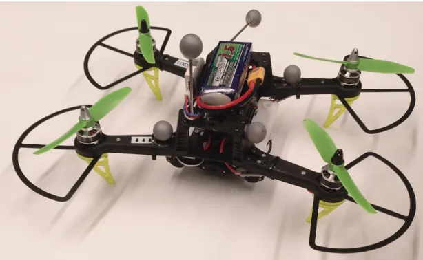
Figure 2-5. Quadrotor vehicle used for the dynamic landing experiments.

2.3

Experimental Results

In this section, the experimental results are presented and analyzed. A video of the flights is available at [66].

2.3.1

Hardware

Static and moving platform landing tests were done (see Fig. 2-1 and Fig. 2-6), both of which had turbulent wind at the landing site from the leaf blowers. The quadrotor used for the hardware experiments (Fig. 2-5) weighs 0.564kg including the 1500mAh 3S battery. It is 36 × 29cm (approximately half the platform size) and its thrust-to-weight ratio is 1.75. The onboard computer is a Qualcomm Snapdragon Flight APQ8074, whose front-facing camera provides 640 × 480 black-and-white images at a rate of 30fps to the AprilTag detection module. Hover tests were carried out to determine ˆ𝑏 in (2.4). To measure the drag coefficient ˆ𝑐 and the bound on its error ˜

𝑐, tests with the quadrotor flying in front of a strong wind were performed, and the accurate pitch angle was obtained by the motion capture system. By balancing forces, the drag could be determined, yielding ˆ𝑐. Additionally, the IMU utils package

[67] was used to compute the Snapdragon’s IMU accelerometer and gyroscope noise density and bias random walk. The Kalibr visual-inertial calibration toolbox then used this IMU intrinsic information to find the camera-IMU transform [68].

2.3.2

Static Platform Experiments

Experiment Setting

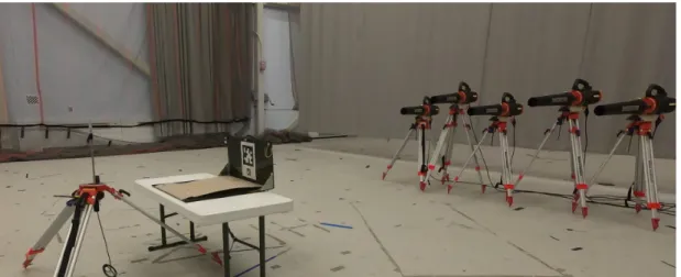
The first set of hardware experiments presents a static platform in front of an array of 5 leaf blowers, as shown in Fig. 2-6. The leaf blowers are set at two different heights and point to the negative 𝑥-direction. The platform is composed of a 60×60cm horizontal plate and a 60×30cm vertical plate, which has attached the tag bundle described in Section 2.2.5. Kraft paper covers the horizontal plate to avoid skidding of the MAV upon landing. As it can be seen in the videos, the kraft paper shakes violently due to the large magnitude of the turbulent wind.

The parameters 𝑣𝑤 and 𝜎 of the turbulent wind were measured at distances 𝑙

from the vertical platform every 0.5m until 𝑙 = 3.5m, which is approximately the tag detection range. For every 𝑙, a measurement of the speed was taken every second for 60s using a high-precision hot-wire anemometer. Figure 2-7 shows the data obtained. Interestingly, at 𝑙 = 0.5m, the mean speed decreases while the standard deviation increases to its maximum value. This might be caused by the vortices that are generated when the flow traverses the vertical platform.

Results

The first set of experiments tested a standard BLSC that does not take into account the turbulent wind generated by the leaf blowers, that is, the factors ˆ𝑓 and 𝐾 only consider the drag generated by the quadrotor’s speed relative to the ground. Figure 2-8 shows the tracking and estimation performance obtained. The quadrotor starts at 𝑝𝑞 = (−3.5, 2.0, 1.3)m, and the platform is located at 𝑝𝑝 = (1.1, −1.1, 0.8)m. As

expected, the tracking performance is poor, and the landing takes a long time: 27.2s since the first tag detection, which occurs at 𝑡𝑑 = 3.3s (indicated with a vertical dashed

Figure 2-6. Leaf blower array in front of the static platform showing the wind measurement pro-cedure. To the left, a hot-wire anemometer on top of a tripod takes measurements to characterize the wind field. To the right, the 5 leaf blowers generate a wind of 6-8 m/s at the landing platform. The kraft paper covering the black horizontal plate flutters rapidly due to the turbulent wind.

Figure 2-7. Mean wind speed (in m/s) from the leaf blowers vs. distance to the vertical platform (with 1 − 𝜎 error bars).

Figure 2-8. Position and velocity tracking and estimation performance of a static platform exper-iment using a BLSC that does not model the turbulence. Wind blowing towards −𝑥 resulting in poor tracking performance in the 𝑥-direction. Vertical dashed lines indicate time of the first tag detection, 𝑡𝑑.

Figure 2-9. Position and velocity tracking and estimation performance of a static platform experi-ment using the disturbance-aware BLSC. The tracking error remains small during the flight.

line). Also note that the platform’s estimation improves after 𝑡𝑑. In the video, the

covariance ellipses for the tag’s 2D position can be seen, and decrease abruptly in size at 𝑡𝑑.

Next, the disturbance-aware BLSC was used with the same initial conditions as in Fig. 2-8 to compare its improvement. The results are shown in Fig. 2-9. It can be seen that the tracking is much better, and it only worsens slightly when the quadrotor is inside the wind field, after the time of the first tag detection 𝑡 = 2.5s. The landing time is just 3.2s (measured since the first tag detection) even in challenging conditions, which is 8.5 times faster compared to the standard BLSC.

2.3.3

Moving Platform Experiments

Experiment Setting

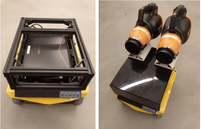
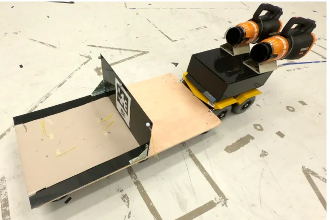
To fully test the approach presented in this chapter, landing experiments on a moving platform were also performed. The Clearpath Jackal was used as the ground vehicle that tows a dolly were the landing platform is mounted (see Fig. 2-1, Fig. 2-10, and Fig. 2-12). On top of the UGV, two cordless leaf blowers were placed on a mount so that the expelled air pointed to the top of the vertical pane of the landing platform, as shown in Fig. 2-11. This provided turbulent air at the landing pad even though the MAV and UGV were not moving very quickly, therefore recreating the conditions found on a vehicle moving at a high speed outdoors. The frame is made of 80/20 T-slot aluminum bars, which are easy to cut and attach together. Therefore, they are useful for rapid prototyping. The mount is covered by 5 Delrin plates that can be attached and detached using velcro. The laptop that controls the ground vehicle is housed inside the mount, and the two cordless leaf blowers are placed on top. The distance from the leaf blowers to the platform is such that this turbulent wind follows the same plot as Fig. 2-7.

Results

A standard BLSC was also tested first for this experiment setting. There was consid-erable tracking error and the quadrotor was not able to land on the platform before the vehicle arrived at the final point (see [66] for details).

The results obtained using the disturbance-aware BLSC are shown in Fig. 2-13. The quadrotor starts at 𝑝𝑞 = (−1.5, 2.7, 0.9)m, and the UGV starts at 𝑝𝑝 =

(−3.9, 0.1, 0.4)m. When the maneuver begins, the UGV is commanded to move at 1m/s and rotate to its right at a rate of 4∘/s. The tag is detected at 𝑡𝑑 = 4.7s, and

the landing time is 6.8𝑠. Note that the quadrotor is at approximately 4m from the moving platform at 𝑡𝑑, a value larger than for the static experiment (1.5m).

Figure 2-10. Landing platform with vertical tag bundle. The MAV can detect the upper tag at a maximum distance of approximately 3.5 m, and the lower tag at a minimum distance of 5 cm. Yellow pieces of thread were added to visualize the wind, as seen in the video [66].

(a) Metal mount on top of the ground vehicle. The strong mount, made of 80/20 T-slot aluminum bars, houses the

ground vehicle’s laptop and supports the leaf blowers.

(b) Two cordless leaf blowers on top of the ground vehicle. Delrin plates cover the frame for aerodynamic and

aesthetic purposes.

Figure 2-11. Assembly of the ground vehicle with two cordless leaf blowers. This systems allows the recreation of turbulent conditions even at small speeds of the ground vehicle.

Figure 2-12. Landing platform on a dolly towed by the UGV, showing two cordless leaf blowers mounted on top of the Clearpath Jackal to recreate the conditions of a vehicle moving outdoors at high speed.

Figure 2-13. Position and velocity tracking and estimation performance of a moving platform ex-periment using the disturbance-aware BLSC. The quadrotor quickly matches the UGV’s velocity and is able to track successfully the planned trajectory.

Chapter 3

Wind Estimation

This chapter is based on [69], a paper submitted to the IEEE/RSJ International Conference on Intelligent Robots and Systems (IROS) 2020.

3.1

Introduction

Disturbance estimation for MAVs is crucial for robustness and safety. This chapter uses novel, bio-inspired airflow sensors to measure the airflow acting on a MAV, and this information is fused in a UKF to simultaneously estimate the three-dimensional wind vector, the drag force, and other interaction forces (e.g. due to collisions, in-teraction with a human) acting on the robot. To this end, a fully model-based and a deep learning-based strategy are presented and compared. The model-based ap-proach considers the MAV and airflow sensor dynamics and its interaction with the wind, while the deep learning-based strategy uses a long short-term memory (LSTM) to obtain an estimate of the relative airflow, which is then fused in the proposed filter. Hardware experiments validate the methods, showing that relative airflow of up to 4 m/s can be accurately estimated, and that drag and interaction forces can be differentiated.

The approach presented in this chapter takes inspiration from the way insects sense airflow [70], which is by measuring the deflections caused by the aerodynamic drag force acting on the appendix of some receptors. By fusing the information of

Figure 3-1. MAV equipped with four bio-inspired airflow sensors used to estimate a three-dimensional wind vector from which aerodynamic drag can be distinguished from other forces (e.g., due to interaction).

four heterogeneous airflow-sensors distributed across the surface of the robot, it is possible to obtain a three-dimensional estimate of the relative velocity of the MAV with respect to the surrounding airflow. This information is then fused in a UKF-based force estimator that uses an aerodynamic model together with the robot’s pose and velocity to predict the wind, the expected drag force, and other interaction forces. To account for the complex aerodynamic interactions between sensors and pro-pellers [71, 72], this model-based approach (based on first-order physical principles) is extended with a data-driven strategy. This strategy employs a recurrent neural net-work (RNN) based on a LSTM netnet-work to provide an estimate of the relative airflow of the robot, which is then fused in the proposed model-based estimation scheme. Experiments show that the approach achieves an accurate estimate of the relative airflow with respect to the robot with velocities up to 4 m/s, and enables interaction forces and aerodynamic drag forces to be distinguished. Based on the experimental results, the model-based and learning-based approaches are compared, highlighting their advantages and disadvantages.

The contributions of this chapter are:

∙ Model- and deep learning-based strategies to simultaneously estimate wind, drag force, and other interaction forces using novel bio-inspired sensors similar to the ones discussed in [73, 74]; and

(a) Bend Labs Digital Flex Sensor (2 axis). (b) Path independence: the sensor’s output Δ𝜃 depends only on the relative angle of its two ends.

Figure 3-2. Bend Labs sensor figures, from [75].

∙ Experimental validation of the approaches, showing that relative airflow of up to 4 m/s is accurately estimated, and interaction force and aerodynamic forces can be distinguished.

3.2

Sensor Design

3.2.1

Initial Sensor Tests

In order to measure the relative wind in 3D affecting a MAV, lightweight and multi-directional sensors need to be used. The two-axis Bend Labs Digital Flex Sensor [75] shown in Fig. 3-2 was used for initial tests and as a proof of concept. It contains two compliant capacitors inside, which are sensitive to strain. When the sensor is deflected, the difference in capacitance from the interior and exterior capacitors is linearly proportional to the deflection angle. Since the total amount of bending is integrated along the length of the sensor, the measured angle ∆𝜃 only depends on the relative angle of the base and the tip of the sensor, a property called path independence [75].

The outputs are, therefore, the roll and pitch deflection angles of the tip of the sensor. It was interfaced via I2C with an Nvidia Jetson TX2 mounted onboard the MAV. Figure 3-3 shows two sensors attached to the hexarotor flown for the hardware

Figure 3-3. Hexarotor with a vertically mounted sensor with fin attachment and wire (center top), and a horizontally mounted sensor (right).

experiments of this chapter. The sensor on the left, mounted vertically, is covered with wire along its length, to make it stiffer, and has a fin appendix made of foam attached to increase its drag coefficient thus amplifying its sensitivity to relative wind. The sensor on the right, mounted horizontally, does not have any modifications. As it can be observed, gravity deflects it downwards.

While this initial testing showed that the relative airflow effects on the deflection angles of the sensors could be observed, their low stiffness, large size, and weight made them impractical to be used for this application. The sensors were largely affected by inertia, and oscillated every time the MAV changed its acceleration.

3.2.2

Sensor Design and Considerations

The previous subsection indicated the need to find a better airspeed sensor. To this end, this thesis adopts sensors based in [73, 74], which are lighter, more economical,

and stiffer compared with the Bend Labs sensors described in Section 3.2.1. The sensors, shown in Fig. 3-4, consist of a base and an easily-exchangeable tip. The base is composed of a magnetic field sensor connected to a conditioning circuit that interfaces with the robot via I2C and a 3D-printed case that encloses the sensor. The tip consists of a planar spring mounted in a 3D-printed enclosure that fits with the base, with a permanent magnet attached to its bottom and a carbon-fiber rod glued on the spring’s top. Eight foam fins are attached on the other end of this rod. When the sensor is subjected to airflow, the drag force from the air on the fins causes a rotation about the center of the planar spring which results in a displacement of the magnet. This displacement is then measured by the magnetic sensor. The fins are placed with even angular distribution in order to achieve homogeneous drag for different airflow directions. Foam and carbon fiber were chosen as the material of the fin structure due to their low density, which is crucial to minimize the inertia of the sensor. Therefore, this sensor has a low response to inertia but a high response to drag, as desired. See [73] for more information about the sensor characteristics and manufacturing procedure.

Due to the complex aerodynamic interactions between the relative airflow and the blade rotor wakes, the sensor placement needs to be chosen carefully [71, 72]. To determine the best locations, short pieces of string were attached both directly on the vehicle and on metal rods extending away from it horizontally and vertically. Then, the hexarotor was flown indoors and it was observed that the pieces of string on top of the vehicle and on the propeller guards were mostly unaffected by the blade rotor wakes. Therefore, these are the two locations chosen to mount the sensors, as seen in Fig. 3-1. They are distributed so that the relative airflow coming from any direction excites at least one sensor (that is, for at least one sensor, the relative airflow is not aligned with its length).

3.2.3

Sensor Measurements

The sensors detect the magnetic field b = (𝑏𝑥, 𝑏𝑦, 𝑏𝑧), but the model outlined in

S

S

S

Foam fins

θ

θ

Carbon-fiber rod

Magnetic sensor

Permanent magnet

Laser-cut spring

3D printed mount

Figure 3-4. Illustration of an airflow sensor and its reference frame S, with the main components labeled.

to the rotation of the carbon fiber rod about the 𝑥 and 𝑦 axes in reference frame 𝑆𝑖.

At the spring’s equilibrium, the rod is straight and b = (0, 0, 𝑏𝑧), where 𝑏𝑧 > 0 if the

magnet’s north pole is facing the carbon-fiber rod. The angles are then

𝜃𝑖 = ⎡ ⎣ 𝜃𝑥,𝑖 𝜃𝑦,𝑖 ⎤ ⎦= ⎡ ⎣ − arctan (𝑏𝑦/𝑏𝑧) arctan (𝑏𝑥/𝑏𝑧) ⎤ ⎦ (3.1)

Note that if the magnet was assembled with the south pole facing upward instead, −b must be used in Eq. (3.1).

3.3

Model-based Approach

This section presents the model-based approach used to simultaneously estimate air-flow, interaction force, and aerodynamic drag force on a MAV. The estimation scheme is based on the UKF [76] approach presented in previous works [22, 24], augmented

with the ability to estimate a three-dimensional wind vector via the relative airflow measurements provided by the whiskers.

A diagram of the most important signals and system-level blocks related to this approach is included in Fig. 3-5.

Reference frame definition The reference frames used in this chapter are an inertial reference frame W, a body-fixed reference frame B attached to the CoM of the robot, and the 𝑖-th sensor reference frame 𝑆𝑖, with 𝑖 = 1, . . . , 𝑁 , as shown in

Fig. 3-4.

3.3.1

MAV Dynamic Model

The MAV considered has a mass 𝑚 and inertia tensor J, and the dynamic equations of the robot can be written as

𝑊p =˙ 𝑊v ˙ R𝐵_𝑊 =R𝐵_𝑊[_𝐵𝜔×] 𝑚_𝑊 ˙v =R𝐵_{𝑊 𝐵}fcmd+_𝑊fdrag+ 𝑚𝑊g +𝑊ftouch J_𝐵𝜔 = −˙ _𝐵𝜔 × J_𝐵𝜔 +_𝐵𝜏cmd (3.2)

where p and v represent the position and velocity of the MAV, respectively, R𝐵 𝑊 is

the rotation matrix representing the attitude of the robot (i.e., such that a vector

𝑊p = R𝐵𝑊 𝐵p), and [×] denotes the skew-symmetric matrix. The vector 𝐵fcmd = 𝐵e3𝑓cmd is the thrust force produced by the propellers along the 𝑧-axis of the body

frame, _𝑊g = −_𝑊e3𝑔 is the gravitational acceleration, and 𝑊ftouch is the interaction

force expressed in the inertial frame. For simplicity, it is assumed that interaction and aerodynamic disturbances do not cause any torque on the MAV, due to its symmetric shape and the fact that interactions (in this thesis’ hardware setup) can only safely happen in proximity of the center of mass of the robot. Vector _𝐵𝜏cmd represents the

torque generated by the propellers and _𝐵𝜔 the angular velocity of the MAV, both expressed in the body reference frame. Here fdrag is the aerodynamic drag force on

Whisker Model Relative Airflow MAV Aerodynamics Model Physical Interaction Disturbance MAV Dynamics Model Aerodynamic Disturbance Position and Attitude Control Pose and Velocity Estimator  Decision Making and Planning

Pose and Velocity Estimate Desired Traj. MAV with Whiskers Motor Speed Whiskers Roll, Pitch Pose

Unscented Kalman Filter

model-based estimation.drawio https://www.draw.io/

Figure 3-5. Diagram of the most important signals used by each step of the proposed model-based approach for simultaneous estimation of wind, drag force, and interaction force.

the robot, expressed as an isotropic drag [77]

𝑊fdrag =(𝜇1v∞+ 𝜇2v∞2 )𝑊ev∞ = 𝑓drag 𝑊ev∞ 𝑊ev∞ = 𝑊v∞ v∞ , where v∞ = ‖𝑊v∞‖ , (3.3)

𝑊v∞ is the velocity vector of the relative airflow acting on the CoM of the MAV

(expressed in the inertial frame)

𝑊v∞ =𝑊vwind−𝑊v, (3.4)

and _𝑊vwind is the velocity vector of the wind expressed in the inertial frame.

3.3.2

Airflow Sensor Model

The 𝑖-th airflow sensor is assumed to be rigidly attached to the body reference frame 𝐵, with 𝑖 = 1, . . . , 𝑁 . The reference frame of each sensor is translated with respect to 𝐵 by a vector _𝐵r𝑆𝑖 and rotated according to the rotation matrix R

𝐵

𝑆𝑖. To derive

a model of the whiskers subject to aerodynamic drag, several assumptions are made.

Each whisker is massless; its tilt angle is not significantly influenced by the accelera-tions from the base 𝐵 (due to the high stiffness of its spring and the low mass of the fins), but is subject to the aerodynamic drag force fdrag,𝑖.

Another assumption made is that each sensor can be modeled as a stick hinged at the base via a linear torsional spring. Each sensor outputs the displacement angle 𝜃𝑥,𝑖 and 𝜃𝑦,𝑖, which correspond to the rotation of the stick around the 𝑥 and 𝑦 axis

of the 𝑆𝑖 reference frame. The aerodynamic drag force acting on the aerodynamic

surface of each sensor _𝑆𝑖fdrag,𝑖 can be expressed as a function of the (small) angular

displacement S_{𝑥,𝑦 𝑆} 𝑖fdrag,𝑖≈ ⎡ ⎣ 0 𝑘𝑖 𝑙𝑖 −𝑘𝑖 𝑙𝑖 0 ⎤ ⎦ ⎡ ⎣ 𝜃𝑥,𝑖 𝜃𝑦,𝑖 ⎤ ⎦= K𝑖𝜃𝑖 (3.5)

where 𝑘𝑖 represents the stiffness of the torsional spring, 𝑙𝑖 the length of the sensor,

and S𝑥,𝑦 = ⎡ ⎣ 1 0 0 0 1 0 ⎤ ⎦ (3.6)

captures the assumption that the aerodynamic drag acting on the 𝑧-axis of the sensor is small (given the fin shapes) and has a negligible effect on the sensor deflection.

Regarding the aerodynamic force acting on a whisker, non-isotropic drag is as-sumed, proportional to the squared relative velocity w.r.t. the relative airflow

𝑆𝑖fdrag,𝑖 = 𝜌 2𝑐𝐷,𝑖A𝑖 ⃦ ⃦_𝑆 𝑖v∞,𝑖 ⃦ ⃦_𝑆 𝑖v∞,𝑖 (3.7)

where 𝜌 is the density of the air, 𝑐𝐷 is the aerodynamic drag coefficient, A𝑖 =

diag([𝑎𝑥𝑦,𝑖, 𝑎𝑥𝑦,𝑖, 𝑎𝑧]⊤) is the aerodynamic section of each dimension, and 𝑐𝐷,𝑖 the

cor-responding drag coefficient. Due to the small horizontal surface of the fin of the sensor, it is assumed that 𝑎𝑧 = 0. The vector 𝑆𝑖v∞,𝑖 is the velocity of the relative

airflow experienced by the 𝑖-th whisker, and expressed in the 𝑖-th whisker reference frame, and can be obtained as

𝑆𝑖v∞,𝑖= R

𝑆𝑖

𝐵 ⊤

where _𝐵v∞

is the relative airflow in the CoM of the robot expressed in the body frame, given by: 𝐵v∞= R𝐵𝑊 ⊤ 𝑊v∞= R𝐵𝑊 ⊤ (_𝑊vwind−𝑊v) (3.9)

3.3.3

Model-based Estimation Scheme

Process Model, State and Output

The MAV dynamic model described in Eq. (3.2) is discretized, augmenting the state vector with the unknown wind _𝑊vwind,k and unknown interaction force𝑊ftouch,𝑘 that

are to be estimated. It is assumed that these two state variables evolve as:

𝑊ftouch,𝑘+1 =𝑊ftouch,𝑘+ 𝜖𝑓,𝑘 𝑊vwind,k+1 =𝑊vwind,k+ 𝜖𝑣,𝑘

(3.10)

where 𝜖𝑓,𝑘 and 𝜖𝑣,𝑘 represent the white Gaussian process noise, with covariances used

as tuning parameters.

The full, discrete time state of the system used for estimation is

𝑥𝑘⊤= {𝑊p𝑘⊤, q𝐵𝑊,𝑘 ⊤ ,_𝑊v𝑘⊤, 𝐵𝜔𝑘⊤,𝑊ftouch,𝑘⊤,𝑊vwind,𝑘⊤} (3.11) where q𝐵

𝑊,𝑘 is the more computationally efficient quaternion-based attitude

represen-tation of the robot, obtained from the rorepresen-tation matrix R𝐵_𝑊,𝑘. The filter output is then

y𝑘⊤= {𝑊ftouch,𝑘⊤,𝑊vwind,𝑘⊤,𝐵v∞,𝑘⊤,𝑊fdrag,𝑘⊤} (3.12)

where _𝑊fdrag,𝑘 is obtained from Eq. (3.3) and Eq. (3.4), and𝐵v∞,𝑘 is obtained from

Measurements and Measurement Model

Two sets of measurements are available asynchronously:

Odometry The filter fuses odometry measurements (position ˆp𝑘, attitude ˆq𝐵𝑊,𝑘,

linear velocity _𝑊v and angular velocityˆ _𝐵𝜔) provided by a cascaded state estimatorˆ

zodometry,𝑘⊤= {𝑊pˆ𝑘⊤, ˆq𝐵𝑊,𝑘 ⊤

,_𝑊vˆ⊤,_𝐵𝜔ˆ⊤} (3.13)

the odometry measurement model is linear, as shown in [22].

Airflow sensors The 𝑁 sensors are sampled synchronously, providing the mea-surement vector zairflowsensor,𝑘⊤= { ˆ𝜃⊤1,𝑘, . . . , ˆ𝜃 ⊤ 𝑁,𝑘} = ˆ𝜃 ⊤ 𝑘 (3.14)

The associated measurement model for the 𝑖-th sensor can be obtained by com-bining Eq. (3.5) and Eq. (3.7)

𝜃𝑖,𝑘 = 𝜌 2𝑐𝐷K𝑖 −1 S𝑥,𝑦A𝑖 ⃦ ⃦_𝑆 𝑖v∞,𝑖,𝑘 ⃦ ⃦_𝑆 𝑖v∞,𝑖,𝑘 (3.15) where _𝑆

𝑖v∞,𝑖,𝑘 is obtained using information about the attitude of the robot q

𝐵 𝑊,𝑘,

its velocity _𝑊v𝑘, and angular velocity 𝐵𝜔𝑘, and the estimated windspeed 𝑊vwind

as described in Eq. (3.8) and Eq. (3.9). The synchronous measurement update is obtained by repeating Eq. (3.15) for every sensor 𝑖 = 1, . . . , 𝑁 .

Prediction and Update Step

Prediction The prediction step (producing the a priori state estimate) [76] is per-formed using the unscented quaternion estimator (USQUE) [78] prediction technique for the attitude quaternion. The process model is propagated using the commanded thrust force 𝑓cmd and torque 𝐵𝜏cmd output of the position and attitude controller on

RNN (Long Short-Term

Memory)

MAV Angular Velocity, Acceleration, Motorspeed Relative Airflow Whiskers Roll,Pitch Whisker Model Relative Airflow MAV Aerodynamics Model Physical Interaction Disturbance MAV Dynamics Model Aerodynamic Disturbance Position and Attitude Control Pose and Velocity Estimator  Decision Making and Planning

Pose and Velocity Estimate Desired Traj. MAV with Whiskers Motor speed Whiskers Roll, Pitch Pose Unscented K a lman Fi lter data-driven-estimation-paper.drawio https://www.draw.io/ 1 of 1 2/29/20, 7:28 PM

Figure 3-6. Signal diagram of the interface between the learning-based and the data-driven ap-proach.

Update The odometry measurement update step is performed using the linear Kalman filter update step [76], while the airflow-sensor measurement update is per-formed via the Unscented Transformation [76] due to the non-linearities in the asso-ciated measurement model.

3.4

Deep Learning-based Approach

This section presents a deep-learning based strategy, which makes use of a RNN based on the LSTM architecture to create an estimate of the relative airflow _𝐵v∞

using the airflow sensors and other measurements available on board of the robot. The complexity in modeling the effects of the aerodynamic interference caused by the airflow between the propellers, the body of the robot and the surrounding air, as observed in the literature [71, 72] and in this chapter’s experimental results, motivates the use of a learning-based strategy to map sensors’ measurement to relative airflow.

3.4.1

Output and Inputs

The output of the network is the relative airflow _𝐵v∞ of the MAV. The inputs to

the network are the airflow sensor measurements 𝜃, the angular velocity of the robot

𝐵𝜔, the raw acceleration measurement from the IMU and the normalized throttle

commanded to the six propellers (which ranges between 0 and 1). The sign of the throttle is changed for the propellers spinning counterclockwise, in order to provide information to the network about the spinning direction of each propeller. The rea-son for the choice of the input is dictated by the derivation from the model-based approach: from Eq. (3.8) and Eq. (3.7) it can be observed that the relative airflow depends on the angle of the sensors and on the angular velocity of the robot. The acceleration from the IMU is included to provide information about hard to model effects, such as the orientation of the body frame w.r.t. gravity (which causes small changes in the angle measured by the sensors), as well as the effects of accelerations of the robot. Information about the throttle and spinning direction of the propellers is instead added to try to capture the complex aerodynamic interactions caused by their induced velocity. Every output and input of the network is expressed in the body reference frame in order to make the network invariant to the orientation of the robot, thus potentially reducing the amount of training data needed.

3.4.2

Network Architecture

An LSTM architecture is employed, which is able to capture time-dependent effects [79, 80], such as, in the case of this thesis, the dynamics of the airflow surrounding the robot and the dynamics of the sensor. A 2-layer LSTM was chosen, with the size of the hidden layer set to 16 (with the input size, 20, and the output size, 3). A single fully connected layer is added to the output of the network, mapping the hidden layer into the the desired output size.

3.4.3

Interface with the Model-based Approach

The UKF treats the LSTM output as a new sensor which provides relative airflow measurements _𝐵vˆ∞, replacing the airflow sensor’s measurement model provided in

Section 3.3. The output of the LSTM is fused via the measurement model in Eq. (3.9), using the unscented transform. A block-diagram representing the interface between the learning-based approach and the model-based approach is represented in Fig. 3-6.

3.5

Experimental Evaluation

3.5.1

System Identification

Drag Force

Estimating the drag force acting on the vehicle is required to differentiate from force due to relative airflow and force due to other interactions with the environment. To this purpose, the vehicle was commanded to follow a circular trajectory at speeds of 1 to 5 m/s, keeping its altitude constant (see Section 3.5.2 for more information about the trajectory generator). In this scenario, the thrust produced by the MAV’s propellers ˆ𝑓thrust is

ˆ

𝑓thrust =

𝑚

cos 𝜑 cos 𝜃𝑔 (3.16)

where 𝑚 is the vehicle’s mass, 𝑔 is the gravity acceleration, and 𝜑 and 𝜃 are respec-tively the roll and pitch angles of the MAV. The drag force is then

ˆ 𝑓drag = (︁ 𝐵ˆfthrust − 𝑚𝐵˙v )︁ ·_𝐵e𝑣 (3.17)

where _𝐵^fthrust = [0, 0, ˆ𝑓thrust], and 𝐵e𝑣 is the unit vector in the direction of the

vehicle’s velocity in body frame. By fitting a second-degree polynomial to the collected data, 𝜇1 = 0.20 and 𝜇2 = 0.07 are obtained (see Eq. (3.3)).

Case 1

Case 2

Top view of a sensor

Figure 3-7. Roll deflection angle of the sensor as a function of the wind speed, for the case where the wind vector is aligned with a fin (1), and the case where it is most misaligned with a fin (2).

Sensor Parameters Identification

The parameters required to fuse the output 𝜃𝑖 of 𝑖-th airflow sensor are its position 𝐵r𝑆𝑖 and rotation R

𝑆𝑖

𝐵 with respect to the body frame B of the MAV, and a lumped

parameter coefficient 𝑐𝑖 mapping the relative airflow𝑆𝑖v∞,𝑖to the measured deflection

angle 𝜃𝑖. The coefficient 𝑐𝑖 = 𝜌₂𝑐𝐷𝑖

𝑎_𝑥𝑦𝑖

𝑘𝑙 can be obtained by re-arranging Eq. (3.15) and

by solving 𝑐𝑖 = ‖𝜃𝑖‖ ⃦ ⃦_𝑆 𝑖v∞,𝑖 ⃦ ⃦ ⃦ ⃦[0 −1 0_{1 0 0}]_𝑆𝑖v∞,𝑖 ⃦ ⃦ (3.18)

and the velocity_𝑆

𝑖v∞,𝑖 is obtained from indoor flight experiments (assuming no wind,

so that _𝑊v∞ = −𝑊v), or by wind tunnel experiments. Wind tunnel experiments

have also been used to validate this chapter’s model choice (quadratic relationship between wind speed and sensor deflection), as show in Fig. 3-7. Furthermore, these experiments also confirmed the assumption on the structure of A𝑖, i.e., the variation

of the sensor’s deflection with respect to the direction of the wind speed is small and therefore it can be considered that 𝑎𝑥 = 𝑎𝑦 = 𝑎𝑥𝑦.

LSTM Training

The LSTM is trained using two different datasets collected in indoor flight. In the first flight the hexarotor follows a circular trajectory at a set of constant velocities ranging from 1 to 5 m/s, spaced of 1 m/s each. In the second data-set the robot is commanded via a joystick, making aggressive maneuvers, while reaching velocities up to 5.5 m/s. Since the robot flies indoor (and thus wind can be considered to be zero) the relative airflow of the MAV_𝐵v∞corresponds to its estimated velocity −_𝐵v, which

is used to train the network. The network is implemented and trained using PyTorch [81]. The data is pre-processed by re-sampling it at 50 Hz, since the inputs of the network used for training have different rates (e.g. 200 Hz for the acceleration data from the IMU and 50 Hz from the airflow sensors). The network is trained for 400 epochs using sequences of 5 samples of length, with a learning rate of 10−4, using the Adam optimizer [82] and the mean squared error (MSE) loss. Unlike the model-based approach, the LSTM does not require any knowledge of the position and orientation of the sensors, nor the identification of the lumped parameter for each sensor. Once the network has been trained, however, it is not possible to reconfigure the position or the type of sensors used.

3.5.2

Implementation Details

System Architecture

The custom-built hexarotor used weighs 1.31 kg. The pose of the robot is provided by a motion capture system, while odometry information is obtained by an estimator running on-board, which fuses the pose information with the inertial data from an IMU. The algorithms run on the onboard Nvidia Jetson TX2 and are interfaced with the rest of the system via ROS. Aerospace Controls Laboratory’s snap stack [83] controls the MAV.

Sensor Driver

The sensors are connected via I2C to the TX2. A ROS node (sensor driver) reads the magnetic field data at 50 Hz and publishes the deflection angles as in Eq. (3.1). Slight manufacturing imperfections are handled via an initial calibration of offset angles. The sensor driver rejects any measured outliers by comparing each component of b with a low-pass filtered version. If the difference is large, the measurement is discarded, but the low-pass filter is updated nevertheless. Therefore, if the sensor deflects very rapidly and the measurement is incorrectly regarded an outlier, the low-pass filtered b quickly approaches the true value and consequent false positives do not occur.

Figure 3-8. Comparison of the relative velocity estimated by the model based (UKF) and the learning-based (LSTM) approaches. The assumption is that the ground truth (GT) is given by the velocity of the robot.

Trajectory Generator

A trajectory generator ROS node commands the vehicle to follow a circular path at different constant speeds or a line trajectory between two points with a maximum desired velocity. This node also handles the finite state machine transitions: take off,

flight to the initial position of the trajectory, execution of the trajectory, and landing where the vehicle took off. This trajectory generator is used to identify the drag coefficient of the MAV (see Section 3.5.1), to collect data for training, and to execute the experiments described below.

3.5.3

Relative Airflow Estimation

For this experiment, the vehicle was commanded with a joystick along the flight space at different speeds, to show the ability of the approach to estimate the relative airflow. Since the space is indoors (no wind), it is assumed that the relative airflow is opposite to the velocity of the MAV. Thus, the velocity of the MAV (obtained from a motion capture system) is compared to the opposite relative airflow estimated via the model-based strategy and the deep-learning based strategy.

Figure 3-8 shows the results of the experiment. Each subplot presents the velocity of the vehicle in body frame. The ground truth (GT) in red is the MAV’s speed obtained via the motion capture system, the green dotted line represents the relative airflow velocity in body frame −_𝐵v∞as estimate via the deep-learning based strategy

(LSTM), and the blue dashed line represents −_𝐵v∞ as estimated by the the fully

model-based strategy (UKF). The root mean squared errors of the UKF and LSTM’s estimation for this experiment are shown in Table 3.1. The results demonstrate that both approaches are effective, but show that the LSTM is more accurate.

3.5.4

Wind Gust Estimation

To demonstrate the ability to estimate wind gusts, the vehicle was flown in a straight line commanded by the trajectory generator outlined in Section 3.5.2 along the diago-nal of the flight space while a leaf blower was pointing approximately to the middle of this trajectory. Figure 3-9 shows in red the estimated wind speed of the UKF drawn at the 2D position where this value was produced, and in green the leaf blower pose obtained with the motion capture system. As expected, the wind speed is increased in the area affected by the leaf blower.

Figure 3-9. In this plot the vehicle is flown in a straight line at high speed, from left to right, while a leaf blower (shown in black) aims at the middle of its trajectory. The red arrows indicate the intensity of the estimated wind speed.