CORADD: Correlation Aware Database Designer for Materialized Views and Indexes

CORADD: Correlation Aware Database

Designer for Materialized Views and Indexes

The MIT Faculty has made this article openly available.

Please share

how this access benefits you. Your story matters.

Citation

Hideaki Kimura, George Huo, Alexander Rasin, Samuel Madden,

and Stanley B. Zdonik. 2010. CORADD: correlation aware database

designer for materialized views and indexes. Proc. VLDB Endow. 3,

1-2 (September 2010), 1103-1113.

As Published

http://dl.acm.org/citation.cfm?id=1920979

Publisher

Association for Computing Machinery (ACM)

Version

Author's final manuscript

Citable link

http://hdl.handle.net/1721.1/73500

Terms of Use

Creative Commons Attribution-Noncommercial-Share Alike 3.0

CORADD: Correlation Aware Database Designer for

Materialized Views and Indexes

Hideaki Kimura

George Huo

Alexander Rasin Samuel Madden Stanley B. Zdonik

Brown University Google, Inc. Brown University MIT CSAIL Brown University

hkimura@cs.brown.edu ghuo@google.com alexr@cs.brown.edu srmadden@mit.edu sbz@cs.brown.edu

ABSTRACT

We describe an automatic database design tool that exploits corre-lations between attributes when recommending materialized views (MVs) and indexes. Although there is a substantial body of related work exploring how to select an appropriate set of MVs and indexes for a given workload, none of this work has explored the effect of correlated attributes (e.g., attributes encoding related geographic information) on designs. Our tool identifies a set of MVs and secondary indexes such that correlations between the clustered attributes of the MVs and the secondary indexes are enhanced, which can dramatically improve query performance. It uses a form of Integer Linear Programming (ILP) called ILP Feedback to pick the best set of MVs and indexes for given database size constraints. We compare our tool with a state-of-the-art commercial database designer on two workloads, APB-1 and SSB (Star Schema Benchmark—similar to TPC-H). Our results show that a correlation-aware database designer can improve query performance up to 6 times within the same space budget when compared to a commercial database designer.

1.

INTRODUCTION

Correlations are extremely common in the attributes of real-world relational datasets. One reason for this is that databases tend to use many attributes to encode related information; for example, area codes, zip codes, cities, states, longitudes, and latitudes all encode spatial data, using slightly different representations, and these attributes are highly correlated (e.g., a given city name usually occurs in only one or two states.) Similar cases occur in many applications; for example, in a retail database, there might be products (e.g., cars) with manufacturers and models. In the case of cars, a given model is likely made by only one manufacturer (e.g., Ford Escape) for a particular set of years (2000–2009) in a particular set of countries (US), yet these are represented by four different attributes in the database. Correlations also occur due to natural relationships between data; for example, in a weather database, high humidity and high temperatures are correlated, and sunny days are also correlated with hot days. Many other examples are described in recent related work [3, 7, 11].

Previous work has shown that the presence of correlations between different attributes in a relation can have a significant impact on query performance [7, 11]. If clustered index keys are well-correlated with secondary index keys, looking up values on the secondary index may be an order of magnitude faster than the uncorrelated case. As a simple example, consider the correlation between city names and state names in a table People (name, city,

Permission to make digital or hard copies of all or part of this work for personal or classroom use is granted without fee provided that copies are not made or distributed for profit or commercial advantage and that copies bear this notice and the full citation on the first page. To copy otherwise, to republish, to post on servers or to redistribute to lists, requires prior specific permission and/or a fee. Articles from this volume were presented at The 36th International Conference on Very Large Data Bases, September 13-17, 2010, Singapore.

Proceedings of the VLDB Endowment,Vol. 3, No. 1

Copyright 2010 VLDB Endowment 2150-8097/10/09... $ 10.00.

state, zipcode, salary) with millions of tuples. Suppose we have a secondary index on city names and our query determines the average salary in “Cambridge,” a city in both Massachusetts and in Maine. If the table is clustered by state, which is strongly correlated with city name, then the entries of the secondary index will only point to a small fraction of the pages in the heap file (those that correspond to Massachusetts or Maine.) In the absence of correlations, however, the Cantabrigians will be spread throughout the heap file, and our query will require reading many more pages (of course, techniques like bitmap scans, indexes with included columns and materialized views can also be used to improve performance of such queries.) Thus, even if we run the same query on the same secondary index in the two cases, query performance can be an order of magnitude faster with a correlated clustered index. We note that such effects are most significant in OLAP (data-warehouse) applications where queries may scan large ranges, in contrast to OLTP databases that tend to perform lookups of single-records by primary keys.

Moreover, such correlations can be compactly represented if attributes are strongly correlated [3, 11]. For example, in [11], we show that by storing only co-occurring distinct values of the clustered and secondary index keys, the secondary index can be dramatically smaller than conventional dense B+Trees, which store one entry per tuple rather than one tuple per distinct value.

This means that, by selecting clustered indexes that are well-correlated with predicated attributes, we can reduce the size and improve the performance of secondary indexes built over those attributes. In many cases, these correlations make secondary index plans a better choice than sequential scans.

Although previous work has shown the benefit of correlations on secondary index performance, it has not shown how to au-tomatically select the best indexes for a given workload in the presence of correlations. Conversely, previous work on automated database design has not looked at accounting for correlations. Hence, in this work, we introduce a new database design tool named CORADD (CORrelation Aware Database Designer) that is able to take into account attribute correlations. CORADD first discovers correlations among attributes and then uses this information to enumerate candidate materialized views (MVs) and clustered indexes over them, selecting a set of candidates that offer good query performance in the presence of correlations. To select an optimal set of MVs within a given space budget, CORADD chooses amongst the candidates using an optimized integer lin-ear programming (ILP) technique called ILP Feedback. Finally, it builds compressed secondary indexes on the MVs that take advantage of the strong correlations, offering good performance especially over warehouse-style workloads that can benefit from such indexes. In summary, our contributions include:

• An MV candidate generation method based on query group-ing, which identifies groups of queries that benefit from the same MV as a result of correlations;

• Techniques to identify the best clustered attributes for candi-date MVs to maximize the benefit from correlations; • An MV candidate selection method based on integer linear

programming and ILP Feedback;

• An implementation and evaluation of CORADD on two data-warehouse benchmarks (SSB [15] and APB-1 [14]), showing that CORADD obtains up to a factor of 6 performance improvement in comparison to a leading commercial product that does not consider correlations.

The rest of the paper is organized as follows. Section 2 summarizes related work on correlations and automatic database designtools. Section 3 describes the architecture of CORADD. Section 4 describes methods to generate candidate MV designs that exploit correlations. Section 5 describes our ILP formulation to pick candidate objects within a given space budget. Section 6 describes the ILP Feedback method to adaptively adjust candidate generation. Section 7 experimentally compares CORADD with a commercial database designer. Finally, Section 8 concludes.

2.

BACKGROUND AND RELATED WORK

Automatically creating a set of database objects to improve query performance is a well-studied problem in the physical database design literature [1, 5, 16]. Most related work takes a query workload as input, enumerates candidate database objects that potentially speed up queries, evaluates the query performance of the objects and then selects objects to materialize.

Most previous work takes a space budget constraint as input to restrict the size of the materialized database objects for two reasons. First, storage is a limited resource. Second, and more importantly, the size of the database is directly linked to its maintenance costs. The cost of inserts or updates rapidly grows as the size of the database grows because additional database objects cause more dirty pages to enter the buffer pool, leading to more evictions and subsequent page writes to disk (Appendix A-3 reproduces an experiment from [11] that demonstrates this effect).

2.1

Exploiting Correlations

Many previous researchers have noted that it is important for query processors to be able to take into account correlations [3, 7, 9, 11]. Chen et al. [7] observed that the performance of secondary indexes in data warehousing applications is substantially affected by correlations with clustered indexes. Their Adjointed Dimension Column Clustering aims to improve the performance of queries in a star schema by physically concatenating the values of commonly queried dimension columns that have restrictions into a new fact table, and then creates a clustered index on that concatenation. They report a 10 times or more speed-up when an appropriate clustered index is selected. In [11], we developed an analytic query cost model that exploits correlations based on a similar observation, which we use to estimate query costs in this paper. Details of the cost model are in [11]. We reproduce the details of the model in Section A-2 for the readers’ convenience; in short, the cost of a range scan via a secondary index is proportional to the number of distinct values of the clustered index to be scanned. When the secondary index is well-correlated with the clustered index, this number will be small and cost will be low; when it is uncorrelated, this value will be large and cost will be high (close to a sequential scan.) We will refer to this as our cost model in the rest of the paper. BHUNT [3], CORDS [9], and our previous work [11] discover and exploit correlations in databases. All three use random sampling to find correlations and find many usable correlations across a range of real and synthetic data sets. BHUNT represents discovered correlations as bumps and exception tables and uses these to rewrite queries. Microsoft SQLServer’s datetime correla-tion optimizacorrela-tion1_{also stores correlations and uses them to rewrite} 1_{http://msdn.microsoft.com/en-us/library/}

ms177416(SQL.90).aspx

queries involving dates. In [11], we developed Correlation Maps (CMs) that use a similar but more general approach; CMs are a type of secondary index that store the clustered index values with which each value of a secondary attribute co-occurs. Then, lookups on the secondary attribute can be performed by scanning the co-occurring clustered attribute values. CMs are thus very compact, as they are a distinct value to distinct value mapping, and can be quite efficient for range queries if the secondary attributes are correlated with a clustered attribute, co-occurring with only a few values.

All of these techniques show that properly clustered primary indexes can improve secondary index performance, but none auto-matically select the best combination of clustered and unclustered designs to maximize query performance. Previous work [3, 7, 9] does not describe how to search for beneficial correlations, and ours [11] only shows how to select beneficial CMs given a clus-tering (i.e., it does not search for a beneficial clusclus-tering.)

2.2

Candidate Selection

Given a set of candidate database objects (MVs and indexes), a database designer must choose a set of objects to materialize with the goal of maximizing overall query performance within the space budget. Previous work proposed two different types of selection algorithms: heuristic and optimal. Heuristic algorithms [1, 5] (e.g., Greedy(m,k) [5]) often choose a suboptimal set of MVs by making greedy decisions. On the other hand, optimal algorithms like integer linear programming (ILP) [16] choose an optimal set in potentially exponential time by exploiting combinatorial optimization techniques. We take the latter approach, further improving the ILP approach from [16] in three ways. First, we improve the ILP structure to account for clustered indexes, of which there is only one per table or MV. Next, we propose to use and evaluate a new ILP-related optimization, ILP Feedback (see Section 6). Lastly, we formulate the design problem so that we do not need to relax integer variables to linear variables, which reduces the error of our approach in comparison to [16].

3.

SYSTEM OVERVIEW

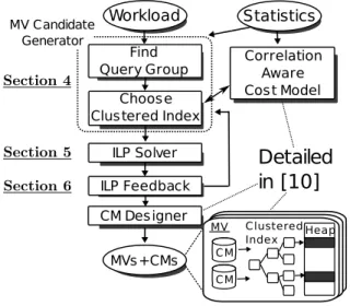
We now describe the design of CORADD, beginning with a system overview. The goal of CORADD is to produce a database design within a given space budget that executes a query workload as quickly as possible – the same goal as previous work [1, 16] – except that we seek a correlation-aware design, The architecture of CORADD is shown in Figure 1. In a nutshell, our design strategy is to choose MVs whose clustered index is well-correlated with attributes predicated in a workload when our cost model identifies cases where such MVs perform significantly better than uncorrelated counterparts.

First, a database workload, expressed as a list of queries that we expect to be executed by the system, is fed into the MV Candidate Generator(Section 4), which produces a set of MVs. In CORADD, an MV design consists of a query group and a clustered index. The query group determines queries the MV can serve and attributes the MV contains. The MV Candidate Generator first selects query groups based on the similarity of their predicates and target attributes, taking into account correlations between those attributes. These query groups are the basis for candidate MV designs, but they do not have clustered indexes at this point. Then, the module produces clustered index designs for the MVs that will take advantage of correlations.

Next, the ILP Solver (Section 5) selects a subset of the candidate MVs that fit in a given space budget and maximize the performance of the system. As described in Section 2, a space budget is also used as a proxy for update cost, allowing CORADD to maximize read query performance subject to constraints on update performance

ILP Solver ILP Feedback Workload Find Query Group Choose Clustered Index MVs+CMs Statistics Correlation Aware Cost Model CM Designer MV Candidate Generator

Detailed

in [10]

Figure 1: CORADD architecture overview

or space. We formulate the problem as an integer linear program (ILP), and use an ILP solver to find an optimal solution.

Third, ILP Feedback (Section 6) sends hints back to the MV Candidate Generatorto improve both query grouping and clustered index design. This module is inspired by the combinatorial optimization technique called Column Generation (CG) [13] and provides an efficient way to explore the design space without con-sidering an exponential number of candidate designs. Specifically, the feedback module iteratively selects additional candidate MVs derived from the previous ILP solution and re-solves the ILP to further improve the quality of MV designs.

Finally, the CM Designer we developed in [11] builds CMs on the MVs that are able to exploit correlations between the clustered key and secondary attributes in the MV. Since a CM serves as a secondary index, the output of this stage is a complete database design that is able to answer queries over both clustered and secondary attributes efficiently. For the readers’ convenience, a summary of the operation of the CM Designer is reproduced in the Appendix. Although we have chosen to describe our approach in terms of CMs, CORADD can also work with other correlation-aware secondary index structures like BHUNT [3] and SQLServer’s date correlation feature.

4.

MV CANDIDATE GENERATOR

The MV Candidate Generator produces an initial set of pre-joined MV candidates, later used by the ILP Solver. Since the number of possible MVs is exponential, the goal of this module is to pick a reasonable number of beneficial MVs for each query. We then use an ILP solver (see Section 5) to select a subset of these possible MVs that will perform best on the entire query workload.

As discussed in Section 2, secondary indexes that are more strongly correlated with the clustered index will perform better. In generating a database design, we would like to choose MVs with correlated clustered and secondary indexes because such MVs will be able to efficiently answer range queries or large aggregates over either the clustered or secondary attributes. Without correlations, secondary indexes are likely to be of little use for such queries. As an added benefit, correlations can reduce the size of secondary indexes, as described in Section 2.1.

A naive approach would be to choose an MV for each query (a dedicated MV) which has a clustered index on exactly the attributes predicated in the query. Such an MV could be used to answer the query directly. However, this approach provides no sharing of MVs across groups of queries, which is important when space is limited. The alternative, which we explore in this paper, is to choose shared MVs that use secondary indexes to cover several queries that have predicates on the same unclustered attributes. We also compare to

Table 1: Selectivity vector of SSB

year yearmonth weeknum discount quantity

Q1.1 0.15 1 1 0.27 0.48

Q1.2 1 0.013 1 0.27 0.20

Q1.3 0.15 1 0.02 0.27 0.20

Strength(yearmonth → year)=1

Strength(year → yearmonth)=0.14

Strength(weeknum → yearmonth)=0.12

Strength(yearmonth → year,weeknum)=0.19

Table 2: Selectivity vector after propagation

year yearmonth weeknum year,weeknum

Q1.1 0.15 0.15(=0.15

1 ) 1 0.15

Q1.2 0.15(=0.013

0.14) 0.013 0.11(=0.0130.12) 0.0162

Q1.3 0.15 0.015(=0.0028_0.19 ) 0.02 0.0028

the naive approach with our approach in the experimental section. The key to exploiting correlations between clustered and sec-ondary indexes in a shared MV is to choose a clustered index that is well-correlated with predicates in the queries served by the MV. Given such a clustered index, secondary indexes are chosen by the CM Designer [11] which (at a high level) takes one query at a time, applies our cost model to every combination of attributes predicated in the query and chooses the fastest combination of CMs to create within some space budget for the query.

Because CMs are faster and smaller when they are correlated with the clustered index, the CM Designer naturally selects the most desirable CMs as long as CORADD can produce a clustered index that is well-correlated with the predicates in a query group.

To find such clustered indexes, CORADD employs a two-step process. First, it selects query groups that will form MV candidates by grouping queries with similar predicates and target attributes. Next, it produces clustered index designs for each MV candidate based on expected query runtimes using a correlation-aware cost model. It also produces clustered index designs for fact tables, considering them in the same way as MV candidate objects.

4.1

Finding Query Groups

We group queries based on the similarity of their predicates and target attributes. Because each MV can have only one clustered index, an MV should serve a group of queries that use similar predicates in order to maximize the correlation between the attributes projected in the MV. We measure the similarity of queries based on a selectivity vector.

4.1.1

Selectivity Vector

For a query Q, the selectivity vector of Q represents the selectiv-ities of each attribute with respect to that query. Consider queries Q1.1, Q1.2, and Q1.3 in the Star Schema Benchmark [15] (SSB), a TPC-H like data warehousing workload, with the following pred-icates that determine the selectivity vectors as shown in Table 1. For example, the selectivity value of 0.15 in the cell (Q1.1, year) indicates that Query 1.1 includes a predicate over year that selects out 15% of the tuples in the table. The vectors are constructed from histograms we build by scanning the database.

Q1.1: year=1993 & 1≤discount≤3 & quantity<25

Q1.2: yearmonth=199401 & 4≤discount≤6 & 26≤quantity≤35

Q1.3: year=1994 & weeknum=6 &

5≤discount≤7 & 26≤quantity≤35

Note that the vectors do not capture correlations between at-tributes. For example, Q1.2 has a predicate yearmonth=199401, which implies year=1994; thus, Q1.2 actually has the same selectivity on year as Q1.3. To adjust for this problem, we devised a technique we call Selectivity Propagation, which is applied to the vectors based on statistics about the correlation between attributes. We adopt the same measure of correlation strength as CORDS [9], namely, for two attributes C1and C2, with |C1| distinct values of C1

1 Q1.1 150MB 1 Q1.2 160MB 2 Q3.4 290MB Benefit Queries Covered

Size

2 Q1.1, Q1.2

170MB

3 Q1.2, Q3.4 400MB

Figure 2: Overlapping target attributes and MV size

|C1|

|C1C2| where a larger value (closer to 1) indicates a stronger

correlation. To measure the strength, we use Gibbons’ Distinct Sampling [8] to estimate the number of distinct values of each attribute and Adaptive Estimation (AE) [4] for composite attributes, as in CORDS [9] and our previous work [11] (see Appendix for the details of cardinality estimation). Using these values, we propagate selectivities by calculating, for a relation with a column set C:

selectivity(Ci)= min j

selectivity(Cj)

strength(Ci→ Cj)

!

For each query, we repeatedly and transitively apply this formula to all attributes until no attributes change their selectivity.

Table 2 shows the vectors for SSB after propagation. Here, yearmonthperfectly determines year, so it has the same selec-tivity as year in Q1.1. On the other hand, year in Q1.2 does not determine yearmonth perfectly (but with a strength 0.14). Thus, the selectivity of year falls with the inverse of the strength. Put another way, year does not perfectly determine yearmonth, as each year co-occurs with 12 yearmonth values. Each year value co-occurs with more distinct values of yearmonth. CORADD also checks the selectivity of multi-attribute composites when the determined key is multi-attribute (i.e. year, weeknum in Q1.3).

4.1.2

Grouping by

-means

Our next step is to produce groups of queries that are similar, based on their selectivity vectors. To do this, we use Lloyd’s k-means[12] to group queries. k-means is a randomized grouping algorithm that finds k groups of vectors, such that items are placed into the group with the nearest mean. In our case, the distance function we use is [v1, v2] =

q P

ai∈A(v1[ai] − v2[ai])

2_{where A is}

the set of all attributes and viis the selectivity vector of query i. We

also used k-means++ initialization [2] to significantly reduce the possibility of finding a sub-optimal grouping at a slight additional cost. After grouping, each query group forms an MV candidate that contains all of the attributes used in the queries in the group. These kmost similar groups are fed into the next phase, which computes the best clustering for each group (see Section 4.2).

CORADD considers queries on different fact tables separately. Hence, the candidate generator runs k-means for each fact table with every possible k-value from 1 to the number of workload queries over that fact table. This method assumes each query accesses only one fact table. When a query accesses two fact tables, we model it as two independent queries, discarding join predicates for our selectivity computation.

We studied several other distance metrics and query grouping approaches with different vectors (e.g., inverse of selectivity) but found that the above method gave the best designs. We also note that, because query groups are adaptively adjusted via ILP feedback(see Section 6) it is not essential for our grouping method to produce optimal groups.

4.1.3

Target Attributes and Weight

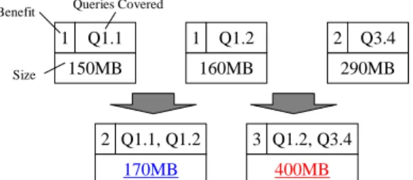
As described so far, our grouping method only takes into account predicate selectivities. It is also important to consider which target attributes (i.e., attributes in the SELECT list, GROUP BY, etc) an MV must include in order to answer queries. Consider the

following queries from SSB [15]; they have similar selectivity vectors because they directly or indirectly predicate on year. However, Q1.2 and Q3.4 have very different sets of target attributes while Q1.1 and Q1.2 have nearly the same set.

Q1.1: SELECT SUM (price*discount)

WHERE year=1993 & 1≤discount≤3 & quantity<25

Q1.2: SELECT SUM (price*discount) WHERE yearmonth= 199401 & 4≤discount≤6 & 26≤quantity≤35 Q3.4: SELECT c city, s city, year, sum(revenue)

WHERE yearmonthstr= ‘Dec1997’

& c city IN (‘UK1’, ‘UK5’) & s city IN (‘UK1’, ‘UK5’)

Now, suppose we have the MV candidates with the sizes and hypothetical benefits shown in Figure 2. An MV candidate cover-ing both Q1.1 and Q1.2 is not much larger than the MVs covercover-ing each query individually because the queries’ target attributes nearly overlap, while an MV candidate covering both Q1.2 and Q3.4 becomes much larger than MVs covering the individual queries. Although the latter MV may speed up the two queries, it is unlikely to be a good choice when the space budget is tight.

To capture this intuition, our candidate generator extends the selectivity vectors by appending an element for each attribute that is set to 0 when the attribute is not used in the query and to bytesize(Attr) × α when it is used. Here, bytesize(Attr) is the size to store one element of Attr (e.g., 4 bytes for an integer attribute) and α is a weight parameter that specifies the importance of overlap and thus MV size. Candidates enumerated with lower α values are more likely to be useful when the space budget is large; those with higher α will be useful when the space budget is tight. When we run k-means, we calculate distances between these extended selectivity vectors, utilizing several α values ranging from 0 to 0.5. We set the upper bound to 0.5 because we empirically observed that α larger than 0.5 gave the same designs as α= 0.5 in almost all cases. The final set of candidate designs is the union of the MVs produced by all runs of k-means; hence, it is not important to find α precisely.

4.2

Choosing a Clustered Index

The next step is to design a clustered index for each of the query groups produced by k-means. The groups produced in the previous steps consist of similar queries that are likely to have a beneficial clustered index, but k-means provides no information regarding what attributes should form the clustered index key. By pairing clustered indexes with query groups that maximize the performance of the related queries, this step produces a set of MV candidates.

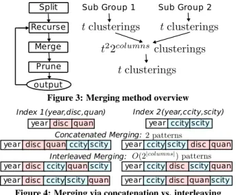
At this point, our goal is not to select the single best design for an MV (this is the job of the ILP described in Section 5), but to enumerate a number (t) of possible designs that may work well for the queries. By choosing t possible clusterings for each MV, we provide a parameterized way for our ILP solver to request additional candidates from which it searches for an optimal design. This is important because it does not require us to fix t a priori; instead, our ILP feedback method interactively explores the design space, running our clustered index designer with different t values. Figure 3 illustrates the operation of our clustered index designer. For an MV of only one query, we can produce an optimal design by selecting the clustered index that includes the attributes predicated by the query in order of predicate type (equality, range, IN) and then in selectivity order. We prefer predicates that are less likely to fragment the access pattern on the clustered key (an equality identifies one range of tuples while an IN clause may point to many non-contiguous ranges). We call such candidates dedicated MVs and observe that they exhibit the fastest performance for the query. For example, a dedicated MV for Q1.2 is clustered on (yearmonth, discount, quantity).

Split Recurse

Merge Prune output

Sub Group 1 Sub Group 2

Figure 3: Merging method overview

year disc quan Index 1(year,disc,quan)

year ccity scity Index 2(year,ccity,scity)

year disc quan ccity scity year ccity scity disc quan

Concatenated Merging:

year disc ccityquanscity year ccity disc scityquan

Interleaved Merging:

year disc ccity scityquan year ccity disc quanscity

Figure 4: Merging via concatenation vs. interleaving into single-query MVs and merge the dedicated clustered indexes, retaining the t clusterings with the best expected runtimes (accord-ing to our cost model). This merg(accord-ing approach is similar to [6], but differs in that we explore both concatenation and interleaving of attributes when merging two clustered indexes as illustrated in Figure 4 while [6] considers only concatenation. Although the approach in [6] is fast, the queries that benefit from correlations with a secondary index usually see no benefit from a concatenated clustered index key. This is because additional clustered attributes become very fragmented, such that queries over them must seek to many different places on disk. We omit experimental details due to space, but we observed designs that were up to 90% slower when using two-way merging compared to interleaved merging.

Additionally, we reduce the overhead of merging by dropping at-tributes when the number of distinct values in the leading atat-tributes becomes too large to make additional attributes useful. In practice, this limits the number of attributes in the clustered index to 7 or 8. Furthermore, order-preserving interleaving limits the search space to 2|Attr|_{index designs, rather than all |Attr|! possible permutations.}

The final output of this module is t clustered indexes for each MV. We start from a small t value on all MVs; later, ILP feedback specifies larger t values to recluster specified MVs, spending more time to consider more clustered index designs for the MVs.

The enumerated MV candidates are then evaluated by the corre-lation aware cost model and selected within a given space budget by ILP Solver described in Section 5.

4.3

Foreign Key Clustering

In addition to selecting the appropriate clustering for MVs, it is also important to select the appropriate clustering for base tables in some applications, such as the fact table in data warehouse applications (in general, this technique applies to any table with foreign key relationships to other tables.) In many applications, clustering by unique primary keys (PKs) is not likely to be effective because queries are unlikely to be predicated by the PK and the PK is unlikely to be correlated with other attributes. To speed up such queries, it is actually better to cluster the fact table on predicated attributes or foreign-key attributes [10].

To illustrate this idea, consider the following query in SSB.

Q1.2: SELECT SUM (price*discount)

FROM lineorder, date WHERE date.key=lineorder.orderdate &

date.yearmonth=199401 & 4≤discount≤6 & 26≤quantity≤35

One possible design builds a clustered index on discount or quantity. However, these predicates are not terribly selec-tive nor used by many queries. Another design is to cluster on the foreign key orderdate, which is the join-key on the

Table 3: Symbols and decision variables

M Set of MV candidates (including re-clustering designs). Q Set of workload queries. F Set of fact tables. Rf Set of re-clustering designs for fact table f ∈ F. Rf⊂ M.

m An MV candidate. m= 1, 2, .., |M|. q A query. q = 1, 2, .., |Q|.

S Space budget. sm Size of MV m.

tq,m Estimated runtime of query q on MV m.

pq,r r-th fastest MV for query q. (r1≤ r2⇔ tq,pq,r₁≤ t_q,pq,r

2).

tq,mand pq,rare calculated by applying the cost model to all MVs. xq,m Whether query q is penalized for not having MV m. 0 ≤ xq,m≤ 1

ym Whether MV m is chosen.

dimension date and is indirectly determined by the predicate date.yearmonth=199401. This clustered index applies to the selective predicate and also benefits other queries. To utilize such beneficial clusterings, CORADD considers correlations between foreign keys and attributes in dimension tables. We then evaluate the benefit of re-clustering each fact table on each foreign key at-tribute by applying the correlation-aware cost model. We treat each clustered index design as an MV candidate, implicitly assuming that its attribute set is all attributes in the fact table and the query group is the set of all queries that access the fact table.

Since it is necessary to maintain PK consistency, the fact table requires an additional secondary index over the PK if we re-cluster the table on a different attribute. CORADD accounts for the size of the secondary index as the space consumption of the re-clustered design. While designs based on a new clustered index may not be as fast as a dedicated MV, such designs often speed up queries using much less additional space and provide a substantial improvement in a tight space budget.

The ILP Solver described next treats fact table candidates in the same way as MV candidates, except that it materializes at most one clustered index from the candidates for each fact table.

5.

CANDIDATE SELECTION VIA ILP

In this section, we describe and evaluate our search method to select database objects to materialize from the candidate objects enumerated by the MV Candidate Generator described in the previous section within a given space budget.

5.1

ILP Formulation

We formulate the database design problem as an ILP using the symbols and variables listed in Table 3. The ILP that chooses the optimal design from a given set of candidate objects is:

Objective: minX q         tq,p_q,1+ X r=2...|M| xq,pq,r(tq,pq,r− tq,pq,r−1)         Subject to: (1) ym∈ {0, 1} (2) 1 − r−1 X k=1 ypq,k≤ xq,pq,r≤ 1 (3) X m smym≤ S (4) ∀ f ∈ F : X m∈Rf ym≤ 1

The ILP is a minimization problem for the objective function that sums the total runtimes of all queries. For a query q, its expected runtime is the sum of the runtime with the fastest MV for q (tq,pq,1)

plus any penalties. A penalty is a slow-down due to not choosing a faster MV for the query, represented by the variable xq,m. Condition (1) ensures that the solution is boolean (every MV is either included or is not). Condition (2) determines the penalties for each query by constraining xq,mwith ym. Because this is a minimization problem

and tq,pq,r− tq,pq,r−1 is always positive (as the expected runtimes are

ordered by r), xq,mwill be 0 if m or any faster MV for q is chosen,

otherwise it will be 1. For example, xq,mis 0 for all m when ypq,1= 1

(the fastest MV for query q is chosen). When ypq,2= 1 and ypq,1= 0,

xq,pq,1is 1 and all the other xq,mare 0, thus penalizing the objective

function by the difference in runtime, tq,p_q,2− tq,p_q,1. Condition (3) ensures that the database size fits in the space budget. Condition (4) ensures that each fact table has at most one clustered index.

4 6 8 10 12 14 16 18 20 6 8 10 12 14 16 18

Expected Total Runtime [sec]

Space Budget [GB] Greedy(m,k)

ILP

Figure 5: Optimal versus greedy.

0 100 200 300 400 500 600 700 0 2 4 6 8 10 12 14 16 18 20

ILP Solver Runtime [sec]

#MV Candidates [thousands] Figure 6: LP solver runtime.

0.95 1 1.05 1.1 1.15 1.2 1.25 1.3 1.35 1.4 2 4 6 8 10 12

Total Runtime [/Optimal]

Space Budget [GB] ILP ILP Feedback

Figure 7: ILP feedback improvement. solver. The resulting variable assignment indicates MVs to

ma-terialize (ym = 1) and we determine the MV to use for each query

by comparing the expected runtime of the chosen MVs. We count the size of CMs separately, as described in Section 5.4.

5.2

Comparison with a Heuristic Algorithm

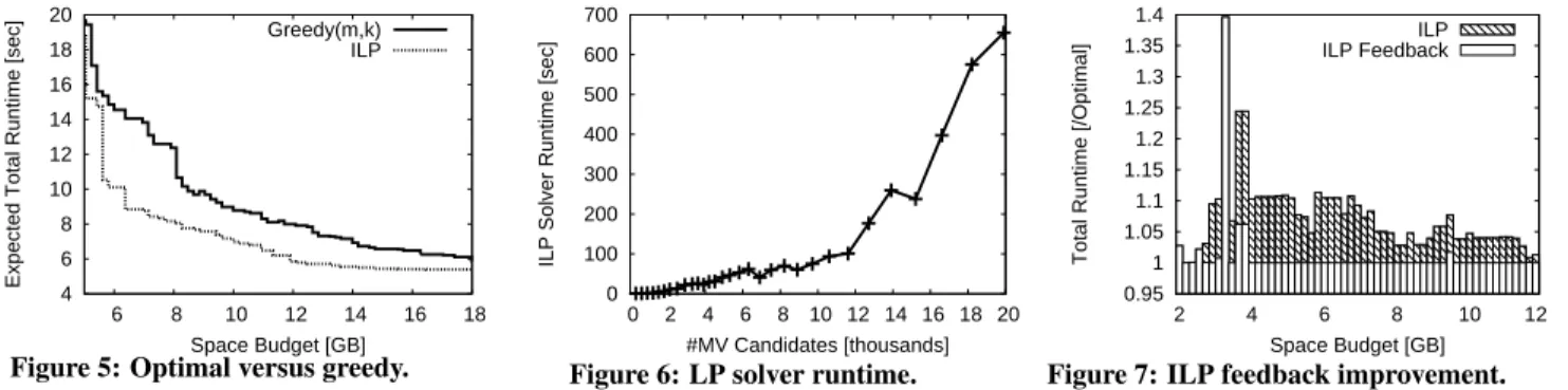
To understand the strength of our optimal solution, we compared our ILP solution against Greedy (m,k) [1, 5], a heuristic algorithm used in Microsoft SQL Server that starts by picking m candidates with the best runtime using exhaustive search and then greedily choosing other candidates until it reaches the space limit or k candidates. As [5] recommends, we used the parameter value m = 2 (we observed that m = 3 took too long to finish). The dataset and query sets are from SSB.

As Figure 5 shows, the ILP solution is 20-40% better than Greedy (m,k) for most space budgets. This is because Greedy (m,k) was unable to choose a good set of candidates in its greedy phase. On the other hand, Greedy (m,k) chooses optimal sets in tight space budgets (0-4GB) where the optimal solutions contain only one or two MVs and the exhaustive phase is sufficient.

5.3

Shrinking the ILP

To quickly solve the ILP, CORADD reduces the number of MVs by removing dominated MVs which have larger sizes and slower runtimes than some other MV for every query that it covers.

For example, MV2 in Table 4 _{MV1 MV2 MV3 . . .} Q1 1 sec 5 sec 5 sec . . . Q2 N/A N/A 5 sec . . . Q3 1 sec 2 sec 5 sec . . . Size 1 GB 2 GB 3 GB . . . Table 4: MV1 dominates MV2, but not MV3. has a slower runtime than MV1

for every query that can use it (Q1 and Q3), yet MV2 is also larger than MV1. This means MV2 will never be chosen be-cause MV1 always performs bet-ter. As for MV3, it is larger than

MV1 and has worse performance on queries Q1 and Q3, but it is not dominated by MV1 because it can answer Q2 while MV1 cannot.

For the SSB query set with 13 queries, CORADD enumerates 1,600 MV candidates. After removing dominated candidates, the number of candidates decreases to 160, which leads to an ILP formulation with 2,080 variables and 2,240 constraints. Solving an ILP of this size takes less than one second.

To see how many MV candidates we can solve for in a reasonable amount of time, we formulated the same workload with a varying numbers of candidates. As Figure 6 shows, our ILP solver produces an optimal solution within several minutes for up to 20,000 MV candidates. Given that 13 SSB queries produced only 160 MV candidates, CORADD can solve a workload that is substantially more complex than SSB as shown in Section 7.

Finally, to account for the possibility that each query appears several times in a workload, CORADD can multiply the estimated query cost by the query frequency when the workload is com-pressed to include frequencies of each query.

5.4

Comparison to other ILP-based designers

Papado et al [16] present an ILP-based database design

formu-lation that has some similarity to our approach. However, our ILP formulation allows us to avoid relaxing integer variables to linear variables, which [16] relies on.

Because compressed secondary indexes are significantly smaller than B+Trees, CORADD can simply set aside some small amount of space (i.e. 1 MB*|Q|) for secondary indexes and then enumerate and select a set of MVs independently of its choice of secondary indexes on them (as in MVFIRST [1]). This gives us more flexibility in the presence of good correlations. As for [16], they must consider the interaction between different indexes; therefore their decision variables represent sets of indexes, which can be expo-nential in number. For this reason, [16] relaxes variables, leading to potentially arbitrary errors. For example, in one experiment, Papado et al converted the relaxed solution to a feasible integer solution by removing one of the indexes, resulting in a 32% lower benefit than the ILP solution. In contrast, our approach substantially reduces the complexity of the problem and arrives at an optimal solution without relaxation.

6.

ILP FEEDBACK

So far, we have described how to choose an optimal set of database objects from among the candidates enumerated by the MV Candidate Generator. In general, however, the final design that we propose may not be the best possible database design, because we prune the set of candidates that we supply to the ILP. In this section, we describe our iterative ILP feedback method to improve candidate enumeration. To the best of our knowledge, no prior work has used a similar technique in physical database design.

Our ILP may not produce the best possible design due to two heuristics in our candidate enumeration approach – query grouping by k-means, and our selection of clustered indexes by merging. Simply adding more query groups or increasing the value of t in the clustered index designer produces many (potentially 2|Q|_{) more}

candidates, causing the ILP solver to run much longer. We tackle this problem using a new method inspired by the combinatorial optimization technique known as delayed column generation, or simply column generation (CG) [13].

6.1

Methodology

Imagine a comprehensive ILP formulation with all possible MV candidates constructed out of 2|Q|_{− 1 query groupings and 2}|Attr|_{− 1}

possible clustered indexes on each of them. This huge ILP would give the globally optimal solution, but it is impractical to solve this ILP directly due to its size. Instead, CORADD uses the MV candidate generator described in Section 4 which generates a limited number of initial query groupings and clustered indexes.

To explore a larger part of the search space than this initial design, we employ two feedback heuristics to generate new can-didates from a previous ILP solution. ILP Feedback iteratively creates new MV candidates based on the previous ILP design and re-solves the ILP until the feedback introduces no new candidates or reaches a time limit set by the user.

The first source of feedback is to expand query groups used in the ILP solution. If the previous solution selects an MV candidate

Query Group Clustering

MV Size

(Budget=200MB)

Figure 8: ILP feedback

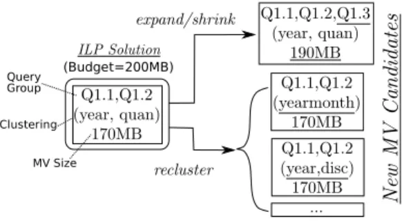
m, expanding m’s query group involves adding a new query (by including that query’s columns in the MV). We consider an expansion with every query not in the query group as long as it does not exceed the overall space budget. This feedback is particularly helpful in tight space budgets, where missing a good query group that could cover more queries is a major cause of suboptimal designs. Additionally, when m is used in the previous solution but is not chosen to serve some query that it covers (because another MV candidate is faster for that query), we also shrink the query group in the hope of reducing the space consumption of m. For example, in Figure 8, the initial ILP solution chooses an MV candidate for the query group (Q1.1, Q1.2) with a clustered index on (year, quantity). As this leaves 30 MB of unused space budget, we add an expanded query group (Q1.1, Q1.2, Q1.3) which does not put the overall design over-budget. If this new candidate is chosen in the next ILP iteration, it will speed up Q1.3.

The second source of feedback is to recluster query groups used in the ILP solution. The size of an MV is nearly independent of its choice of clustered index because the B+Tree size is dominated by the number of the leaf nodes. So, when an MV candidate m is chosen in the ILP solution, a better clustered index on m might speed up the queries without violating the space limit. To this end, we invoke the clustered index designer with an increased t-value in hopes of finding a better clustered index. The intuition is that running with an increased t value for a few MVs will still be reasonably fast. This feedback may improve the ILP solution, especially for large space budgets, where missing a good clustered index is a major cause of suboptimal designs because nearly all queries are already covered by some MV. For example, in the case above, we re-run the clustered index designer for this MV with the increased t and add the resulting MV candidates to the ILP formulation. Some of these new candidates may have faster clustered indexes for Q1.1 and Q1.2.

6.2

ILP Feedback Performance

To verify the improvements resulting from ILP feedback, we compared the feedback-based solution, the original ILP solution, and the OPT solution for SSB. OPT is the solution generated by running ILP on all possible MV candidates and query groupings. We obtained it as a baseline reference by running a simple brute force enumeration on 4 servers for a week. Note that it was possible to obtain OPT because SSB only has 13 queries (213_{− 1= 8191}

possible groups); for larger problems this would be intractable. Figure 7 compares the original ILP solution and the ILP feed-back solution, plotting the expected slowdown with respect to OPT. Employing ILP feedback improves the ILP solution by about 10%. More importantly, the solution with feedback actually achieves OPT in many space budgets. Note that the original ILP solution could incur more than 10% slowdown if SSB had more attributes with more complicated correlations.

As for the performance of ILP feedback, it took the SSB workload 2 iterations to converge and the approach added only 700 MV candidates to the 1,600 original candidates in the ILP, adding 10 minutes to 17 minutes total designer runtime. Therefore,

we conclude that ILP feedback achieves nearly optimal designs without enumerating an excessive number of MV candidates.

7.

EXPERIMENTAL RESULTS

In this section, we study the performance of designs that CORADD produces for a few datasets and workloads, comparing them to a commercial database designer.

We ran our designs on a popular commercial DBMS running on Microsoft Windows 2003 Server Enterprise x64 Edition. The test machine had a 2.4 GHz Quad-core CPU, 4 GB RAM and 10k RPM SATA hard disk. To create CMs in the commercial database, we introduced additional predicates that indicated the values of the clustered attributes to be scanned when a predicate on an unclustered attribute for which an available CM was used (see [11] and Appendix A-1.3 for the details of this technique.)

We compared CORADD against the DBMS’s own designer, which is a widely used automatic database designer based on state-of-the-art database design techniques (e.g., [1, 5].)

To conduct comparisons, we loaded datasets described in the following section into the DBMS, ran both CORADD and the commercial designer with the query workload, and tested each design on the DBMS. We discarded all cached pages kept by the DBMS and from the underlying OS before running each query.

7.1

Dataset and Workload

The first dataset we used is APB-1 [14], which simulates an OLAP business situation. The data scale is 2% density on 10 channels (45M tuples, 2.5 GB). We gave the designers 31 template queries as the workload along with the benchmark’s query distribu-tion specificadistribu-tion. Though CORADD assumes a star schema, some queries in the workload access two fact tables at the same time. In such cases, we split them into two independent queries.

The second dataset we used is SSB [15], which has the same data as TPC-H with a star schema workload with 13 queries. The data size we used is Scale 4 (24M tuples, 2 GB). For experiments in this section, we augmented the query workload to be 4 times larger. The 52 queries are based on the original 13 queries but with varied target attributes, predicates, GROUP-BY, ORDER-BY and aggregate values. This workload is designed to verify that our designer works even for larger and more complex query workloads.

7.2

Results

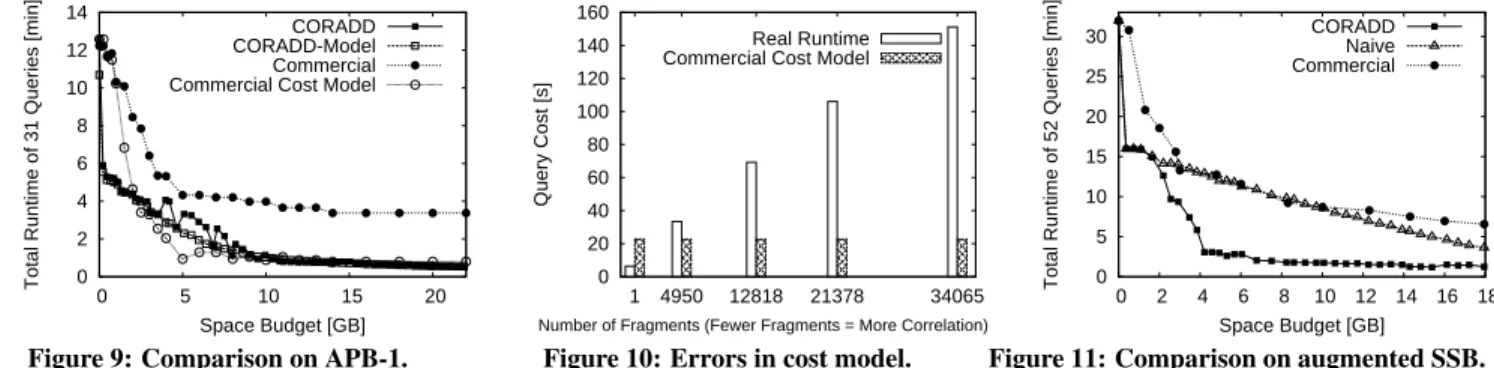
Experiment 1: In the first experiment, we ran designs produced by CORADD and the commercial designer on APB-1. Figure 9 shows the total expected runtime of both designs for each space budget (determined by the cost model) as well as the total real runtime.

The expected runtime of CORADD (CORADD-Model) matched the real runtime (CORADD) very well and, as a consequence, it almost monotonically improves with increased space budgets. Both expected and real runtimes rapidly improved at the 500 MB point where the fact tables are re-clustered to cover queries, and 1 GB to 8 GB points where MVs start to cover queries. After 8 GB where all queries are already covered by MVs, the runtime gradually improves by replacing large MVs with many small MVs that have more correlated clustered indexes. Also at that point, CORADD stops re-clustering the fact table (saving an additional secondary index on the primary key), spending the budget on MVs instead.

Compared with the designs produced by the commercial de-signer (Commercial), our designs are 1.5–3 times faster in tight space budgets (0–8 GB) and 5–6 times faster in larger space bud-gets (8–22 GB). The commercial designer’s cost model estimates the runtime of its designs to be much faster than reality (shown by Commercial Cost Model). The error is up to 6 times and worse in larger space budgets where the designer produces more MVs and indexes.

0 2 4 6 8 10 12 14 0 5 10 15 20

Total Runtime of 31 Queries [min]

Space Budget [GB] CORADD CORADD-Model Commercial Commercial Cost Model

Figure 9: Comparison on APB-1.

0 20 40 60 80 100 120 140 160 1 4950 12818 21378 34065 Query Cost [s]

Number of Fragments (Fewer Fragments = More Correlation)

Real Runtime Commercial Cost Model

Figure 10: Errors in cost model.

0 5 10 15 20 25 30 0 2 4 6 8 10 12 14 16 18

Total Runtime of 52 Queries [min]

Space Budget [GB] CORADD

Naive Commercial

Figure 11: Comparison on augmented SSB. To see where the error comes from, we ran a simple query

using a secondary B+Tree index on SSB Scale 20 lineorder table. We varied the strength of correlation between the clustered and the secondary index by choosing different clustered keys. Here, fewer fragments indicate the correlation is stronger (see Section A-2.2 for more detail). As Figure 10 shows, the commercial cost model predicts the same query cost for all clustered index settings, ignoring the effect of correlations. This results in a huge error because the actual runtime varies by a factor of 25 depending on the degree of correlation.

Due to its lack of awareness of correlations, the commercial designer tends to produce clustered indexes that are not well-correlated with the predicated attributes in the workload queries, causing many more random seeks than the designer expects. CORADD produces MVs that are correlated with predicated at-tributes and hence our designs tend to minimize seeks. Also, our cost model accurately predicts the runtime of our designs. Experiment 2: This experiment is on the augmented (52 queries) SSB. We again ran CORADD and the commercial designer to compare runtimes of the results. This time, we also ran designs produced by a much simpler approach (Naive) than CORADD but with our correlation-aware cost model. Naive produces only re-clusterings of fact tables and dedicated MVs for each query without query grouping and picks as many candidates as possible. Although this approach is simple, it loses an opportunity to share an MV between multiple queries, which CORADD captures via its query grouping and merging candidate generation methods.

As shown in Figure 11, our designs are again 1.5–2 times better in tight space budgets (0–4 GB) and 4–5 times better in larger space budgets (4–18 GB). Even designs produced by Naive approach are faster than the commercial designer’s in tight space budgets (< 3 GB) because it picks a good clustered index on the fact table, and in larger budgets (> 10 GB) because our cost model accurately predicts that making more MVs with correlated clustering indexes will improve the query performance. However, the improvement by adding MVs is much more gradual than in designs of CORADD. This is because Naive uses only dedicated MVs, and a much larger space budget is required to achieve the same performance as designs with MVs shared by many queries via compact CMs.

Finally, we note that the total runtime of CORADD to produce all the designs plotted in Figure 11 was 7.5 hours (22 minutes for statistics collection, an hour for candidate generation, 6 hours for 3 ILP feedback iterations) while the commercial designer took 4 hours. Although CORADD took longer, the runtime is comparable and the resulting performance is substantially better.

8.

CONCLUSIONS

In this paper, we showed how to exploit correlations in database attributes to improve query performance with a given space budget. CORADD produces MVs based on the similarity between queries and designs clustered indexes on them using a recursive merg-ing method. This approach finds correlations between clustered and secondary indexes, enabling fast query processing and also

compact secondary indexes via a compression technique based on correlations. We introduced our ILP formulation and ILP Feedback method inspired by the Column Generation algorithm to efficiently determine a set of MVs to materialize under given space budget.

We evaluated CORADD on the SSB and the APB-1 benchmarks. The experimental result demonstrated that a correlation-aware database designer with compressed secondary indexes can achieve up to 6 times faster query performance than a state-of-the-art commercial database designer with the same space budget.

9.

REFERENCES

[1] S. Agrawal, S. Chaudhuri, and V. Narasayya. Automated selection of materialized views and indexes in SQL databases. In VLDB 2000.

[2] D. Arthur and S. Vassilvitskii. k-means++: The advantages of careful seeding. In SODA 2007.

[3] P. Brown and P. Haas. BHUNT: Automatic discovery of fuzzy algebraic constraints in relational data. In VLDB 2003. [4] M. Charikar, S. Chaudhuri, R. Motwani, and V. Narasayya.

Towards estimation error guarantees for distinct values. In PODS 2000.

[5] S. Chaudhuri and V. Narasayya. An efficient cost-driven index selection tool for Microsoft SQL Server. In VLDB 1997.

[6] S. Chaudhuri and V. Narasayya. Index merging. In ICDE 1999.

[7] X. Chen, P. O’Neil, and E. O’Neil. Adjoined dimension column clustering to improve data warehouse query performance. In ICDE 2008.

[8] P. B. Gibbons. Distinct sampling for highly-accurate answers to distinct values queries and event reports. In VLDB 2001. [9] I. Ilyas, V. Markl, P. Haas, P. Brown, and A. Aboulnaga.

CORDS: automatic discovery of correlations and soft functional dependencies. In SIGMOD 2004.

[10] N. Karayannidis, A. Tsois, T. Sellis, R. Pieringer, V. Markl, F. Ramsak, R. Fenk, K. Elhardt, and R. Bayer. Processing star queries on hierarchically-clustered fact tables. In VLDB 2002.

[11] H. Kimura, G. Huo, A. Rasin, S. Madden, and S. B. Zdonik. Correlation Maps: A compressed access method for exploiting soft functional dependencies. In VLDB 2009. [12] S. Lloyd. Least squares quantization in PCM. IEEE

Transactions on Information Theory, 28(2):129–137, 1982. [13] M. Lubbecke and J. Desrosiers. Selected topics in column

generation. Operations Research, 53(6):1007–1023, 2005. [14] OLAP-Council. APB-1 OLAP Benchmark Release II, 1998. [15] P. O’Neil, E. O’Neil, and X. Chen. The star schema

benchmark (SSB). Technical report, Department of Computer Science, University of Massachusetts at Boston, 2007.

[16] S. Papadomanolakis and A. Ailamaki. An integer linear programming approach to database design. In ICDE 2007.

APPENDIX

A-1.

CORRELATION MAPS

In this section, we describe the correlation map (CM) structure developed in our prior work. This background material is a summary of the discussion in Section 5 and 6 of [11]; we refer the reader to that paper for a more detailed description.

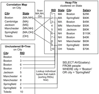
A CM is a compressed secondary index that utilizes correlations between the indexed and clustered attributes. A CM is just a key-value mapping from each unclustered attribute key-value to the set of co-occurring clustered attribute values. The use of CMs in query processing is also straightforward. Figure 12 illustrates an example CM and how it guides the query executor. Here, the secondary B+Tree index on city is a dense structure, containing an entry for every tuple appearing with each city. In order to satisfy the “Boston” or “Springfield” predicate using a standard B+Tree, the query engine uses the index to look up all corresponding rowids.

Heap File clustered on State Unclustered B+Tree on City Toledo 10 9 Springfield Manchester 6 4 3 RID Boston Jackson Manchester 2 1 Springfield Boston 7 City 5 8 Boston Boston Correlation Map on City City State SELECT AVG(salary) FROM people WHERE city = 'Boston' OR city = 'Springfield' 10 OH Toledo $70K $95K 9 OH Springfield $60K 8 NH Manchester MA $40K 7 State Boston MA $110K City Manchester 2 4 Boston $25K 1 $80K NH 6 Jackson Springfield $90K MS MA RID NH Boston $50K $45K Boston 3 Salary 5 MN {MS} Jackson {OH} Toledo {MA,OH} Springfield {MN,NH} Manchester {MA} Cambridge {MA,NH} Boston Scan MA,NH, OH Lookup individual tuples that match

(sorting RIDs) first)

Figure 12: Diagram illustrating an example CM and its use in a query plan, compared to a conventional B+Tree. Reproduced from Figure 4 of [11].

The equivalent CM in this example contains only the unique (city, state) pairs. In order to satisfy the same predicate using a CM, the query engine looks up all possible state values corresponding to “Boston” or “Springfield.” The resulting values (“MA”, “NH”, “OH”) correspond to 3 sequential ranges of rowids in the table. These are then scanned and filtered on the original citypredicate. Notice that the CM scans a superset of the records accessed by the B+Tree, but it contains fewer entries. So, its maintenance costs are low (important for the reasons discussed in Section 2) and it can lead to lower access costs if it remains in memory due to its small size.

A-1.1

Bucketing

CMs further reduce their size via bucketing, compressing ranges of the unclustered or clustered attribute together into a single value. For example, suppose for each city we also store the median income and percentage of workers who are doctors; we build a CM on the attribute income with a clustered index on %-doctors (these attributes are clearly correlated, assuming doctors are wealthy). Given the unbucketed mapping on the left in the example below, we can bucket it into the $10, 000 or 10% intervals shown on the right via truncation:

{$66, 550} → {18.3%} {$73, 420} → {20.1%} {$76, 950} → {25.5%} {$85, 200} → {30.3%} {$89, 900} → {33.8%} {$60, 000 − $70, 000} → {10% − 20%} {$70, 000 − $80, 000} → {20% − 30%} {$80, 000 − $90, 000} → {30% − 40%}

This technique keeps CMs small, although now each CM at-tribute value maps to a larger range of clustered index values which increases the number of pages scanned for each CM lookup.

A-1.2

CM Designer

In [11], we also developed a CM Designer that identifies good attributes on which to build CMs and searches for optimal CM bucketings, finding a balance in the trade-off between index size and false positives. In this section, we briefly present our CM Designer. Though CMs are usually small for correlated attributes, it is important for the CM Designer to consider bucketing them when either attribute is many-valued.

We look at two cases: bucketing the clustered column and bucketing the unclustered column (the “key” of the CM).

To bucket clustered columns, the CM Designer adds a new column to the relation that represents the “bucket ID.” All of the tuples with the same clustered attribute value will have the same bucket ID, and some consecutive clustered attribute values will also have the same bucket ID. The CM then records mappings from unclustered values to bucket IDs, rather than to values of the clustered attribute.

Wider buckets for clustered columns cause CM-based queries to read a larger sequential range of the clustered column (by intro-ducing false positives), increasing sequential I/O reads. However, such bucketing does not increase the number of expensive disk seeks. Thus the CM Designer is not sensitive about the width of the clustered column bucketing and uses a reasonable fixed-width scheme (e.g., 20 pages per bucket ID).

Bucketing unclustered attributes has a larger effect on perfor-mance because merging two consecutive values in the unclustered domain will potentially increase the amount of random I/O the system must perform (it will have to look up additional, possibly non-consecutive values in the clustered attribute). Therefore, the CM Designer considers several possible bucketing schemes for each candidate attribute by building equi-width histograms for different bucket widths from random data samples. The CM Designer then exhaustively tries all possible composite index keys and bucketings of attributes for a given query to estimate the size and performance of the CM, selecting the fastest design within a given space limit (1MB per CM in this paper).

A-1.3

Using CMs

We employ a query rewriting approach to use CMs where we introduce predicates (based on CMs) to exploit correlations in our queries (as in [11] and [3]). If we build a CM on an attribute a, with a clustered attribute c, and a query includes a predicate selecting a set of values va∈ a, then we perform a lookup on the CM to find all

values of vc ∈ c that co-occur with va, and add the predicate c IN

vcto the query. For example, suppose in SSB that c is orderdate

and a is commitdate, and we are running the query:

SELECT AVG(price * discount) FROM lineorder

WHERE commitdate=950101

If commitdate value 19950101 co-ocurs with orderdates 19941229, 19941230, and 19941231, we rewrite the query as:

SELECT AVG(price * discount) FROM lineorder

WHERE commitdate=19950101 AND

Note that query rewriting is just one possible way of forcing the DBMS to utilize clustered indexes. It could be implemented internally in the DBMS thereby obviating the need for query rewrit-ing and further improvrewrit-ing the performance of our designs. We employed the rewriting approach to avoid modifying the DBMS. Section 7.1 of [11] provides more details about the CM system.

A-2.

CORRELATION AWARE COST

MODEL

In this section, we review the correlation-aware cost model we developed in [11] which predicts query performance based on correlations between clustered attributes and predicated attributes indexed by secondary indexes. Because the cost model embraces data correlations, it is substantially more accurate than existing cost models in the presence of strongly correlated attributes. We describe the intuition behind the model in Section A-2.1 and the formal definition in Section A-2.2.

A-2.1

Concepts

Consider the following SSB query on lineorder; suppose that we have a secondary B+Tree index on commitdate.

SELECT AVG(price * discount) FROM lineorder

WHERE commitdate=19950101

Typically, a DBMS processes this query using a sorted in-dex scan which sorts Row IDs (or clustered attribute values in some DBMSs) retrieved from the secondary index and performs a single sequential sweep to access the heap file. In such an access pattern, the I/O cost is highly dependent on how matching tuples scatter in the heap file. For this query, if the clustered attribute is highly correlated with commitdate, then the tuples with commitdate=19950101will likely be located in only a few small, contiguous regions of the heap file and the secondary index scan will be much cheaper than a full table scan; on the other hand, if there are no correlations, these tuples will be spread throughout the table, and the secondary scan will cost about the same as the full table scan.

To illustrate this, in Figure 13 we visualize the distribution of page accesses when performing lookups on the secondary index. This background material is a summary of the discussion in Section 3 of [11], and we refer the reader to that paper for more detail.

Page 0 . . . n

orderdate orderkey

Figure 13: Access patterns in lineorder for a secondary index lookup on commitdate with different clustered attributes.

The figure shows the layout of the lineorder table as a hori-zontal array of pages numbered 1 . . . n. Each black mark indicates a tuple in the table that is read during lookups of three distinct values of commitdate. The two rows represent the cases when the table is clustered on orderdate (top) and orderkey (bottom). The orderdate and commitdate are highly correlated as most products are committed to ship at most a few days after they are ordered, whereas commitdate and orderkey have no correlation. As the figure shows, the sorted index scan only performs three large seeks to reach long sequential groups of pages when the table is clustered on orderdate, while it has to touch almost all areas for orderkey. The effect of this difference on query runtime is striking. We ran the query with both clustering schemes on SSB lineorderScale 20. The uncorrelated case took 150 seconds while the correlated case finished in 6 seconds even though exactly the same operations were performed on the secondary index.

As the result shows, data correlations play a significant role in query runtime. In the next section, we describe the model we have developed to account for these costs.

A-2.2

Cost Model

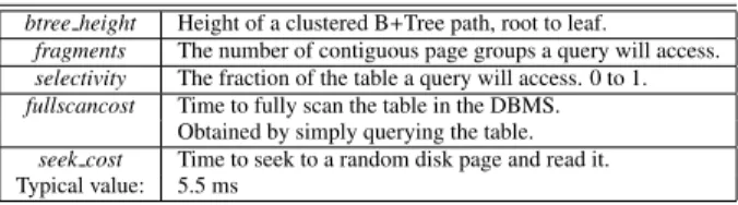
Our correlation-aware cost model is defined in terms of the statistics shown in Table 5, which are collected for each relation. As in [11], we assume that every operation is disk-bound.

cost= cost read + cost seek cost read= fullscancost × selectivity

cost seek= seek cost × fragments × btree height The query cost consists of sequential read cost (cost read) and random seek cost (cost seek). cost seek is determined by the number of fragments the query must visit during a sorted index scan, while cost read is determined by the selectivity, the fraction of the table the query must touch.

Table 5: Statistics used in cost model.

btree height Height of a clustered B+Tree path, root to leaf.

fragments The number of contiguous page groups a query will access. selectivity The fraction of the table a query will access. 0 to 1. fullscancost Time to fully scan the table in the DBMS.

Obtained by simply querying the table. seek cost Time to seek to a random disk page and read it. Typical value: 5.5 ms

A DBMS typically reads several sequential pages together at once, even when it needs only a few tuples in that range (because disk seeks are much more expensive than sequential reads). There-fore, our model considers two tuples placed at nearby positions in the heap file to be one fragment.

Before we can use our cost model, we scan existing tables and calculate the following statistics as described in [11]:

1. Cardinality of each attribute.

2. Statistics about the strength of functional dependencies. 3. Selectivities of predicates in workload queries. 4. Table synopses consisting of random samples.

Additionally, we run the Adaptive Estimator (AE) [4] over random samples on the fly to estimate fragments and selectivity for a given MV design and query. These statistics and random samples can be efficiently maintained under updates by the algorithm Gibbons [8] described. Therefore, the main cost to have these statistics is the database scan, which runs only once at startup.

A-3.

DATABASE SIZE AND MAINTENANCE

COST

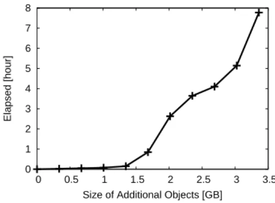
In this section, we demonstrate how the size of the database is directly linked to its maintenance costs. To illustrate this, we ran an experiment where we inserted 500k tuples into the SSB lineorder table while varying the total size of additional database objects (e.g., MVs) in the system (see Section 7 for our experimental setup). The results are shown in Figure 14; as the size of the materialized MVs grows, the cost of 500k insertions grows rapidly. With 3 GB worth of additional MVs, the time to perform the insertions is 67 times slower than with 1 GB of additional MVs. The reason why maintenance performance deteriorates given more objects is that additional objects cause more dirty pages to enter the buffer pool for the same number of INSERTs, leading to more evictions and subsequent page writes to disk. The lineorder table has 2 GB of data while the machine has 4 GB RAM; creating 3 GB of MVs leads to significantly more page writes than 1 GB of MVs.

0 1 2 3 4 5 6 7 8 0 0.5 1 1.5 2 2.5 3 3.5 Elapsed [hour]

Size of Additional Objects [GB]

Figure 14: Cost of 500k insertions.

In Experiment 3 of [11], we observed similar deterioration in update performance as we added more B+Tree indexes while adding more CMs had almost no effects because of their small sizes.

Therefore, despite the decreasing price per gigabyte of storage, space budgets remain an important parameter of database design tools so that data warehousing workloads can be completed within available time limits (e.g., 100k insertions between 12 am and 3 am).

A-4.

PROOF SKETCH OF TERMINATION

OF SELECTIVITY PROPAGATION

In this section, we give a sketch of proof that Selectivity Propa-gationdescribed in Section 4.1 always terminates in finite time.

Let a step be the process of calculating propagated selectivities for all attributes and updating the selectivity vector. At each step, each attribute can be updated by a single parent which gives the minimum selectivity after propagation. The parent could have been updated by its parent (grand parent), but there can not be any cycle in the update path because the strength of functional dependency is always less than one. Thus, the maximum length of an update path is |A| where A is the set of all attributes. Therefore, selectivity propagation terminates at most after |A| steps and each step takes O(|A|2_{), resulting in O(|A|}3_{) computation cost.}

The proof becomes more complex and runtime becomes larger when considering composite functional dependencies (i.e., AB → C) but the main concept above stays the same.

Acknowledgments

We would like to thank Meinolf Sellmann for his help in integrating combinatorial optimizations into CORADD. Samuel Madden was supported by NSF grant IIS-0704424 as well as a grant from SAP Corporation. Hideaki Kimura, Alexander Rasin and Stan Zdonik were supported in part by the NSF, under the grants IIS-0905553 and IIS-0916691.