by
CHRISTOPHER A. DAVIS
B. S. Physics
University of Massachusetts (Amherst)
(1985)
Submitted to the Department of Earth, Atmospheric and Planetary Sciences in partial fulfillment
of the requirements for the degree of
DOCTOR OF PHILOSOPHY IN METEOROLOGY
at the
MASSACHUSETTS INSTITUTE OF TECHNOLOGY May, 1990
© Massachusetts Institute of Technology 1990
All rights reserved
Signature of Author... ... .. ... ...
Dept. of Earth, Atmospheric and Planetary Sciences May, 1990 C ertified by... ... Kerry A. Emanuel Professor of Meteorology Thesis Supervisor Accepted by ... ... ...
Thomas H. Jordan - Chairman Departmental Committee on Graduate Students
1iT i
w990
MIT
ULAaRIES
WITH POTENTIAL VORTICITY by
Christopher A. Davis
Submitted to the Department of Earth, Atmospheric and Planetary Sciences on May 21, 1990 in partial fulfillment of the requirements for the Degree of
Doctor of Philosophy in Meteorology
Abstract
With the assumption of dynamically balanced flow, the structure and development of cyclones may be understood in terms of the distribution and evolution of the interior potential vorticity (PV) and boundary potential temperature (eB) fields. The goals of this observation based diagnostic study are: (1) to document the PV and 0 distribution during four cases of cyclogenesis and quantify the contributions of the observed perturbations of PV and 8B to the circulation of each cyclone (2) to examine the origin of PV and 0B
features comprising the majority of the cyclone perturbation and
(3) to diagnose the influence of condensation on development,
primarily through its effects on the PV distribution.
In each case examined, the initial development is dominated by the growth of a positive eB perturbation. The largest contributor to this growth is the flow associated with upper tropospheric PV anomalies. Lower tropospheric potential vorticity perturbations develop during cyclogenesis just upshear from the region of heaviest stratiform precipitation. Calculations of potential vorticity generation using both the balance equations and station precipitation data indicate that latent heat released in these regions is sufficient to account for the observed changes in low level PV.
Differences among the cases seemed to be smallest at the surface and largest at upper levels. Two cases exhibited large
amplitude upper level waves, the disturbances aloft and at low levels amplified simultaneously. The primary growth phase showed a nearly fixed vertical structure. Positive low level PV anomalies were generated in phase with the OB field and contributed roughly
1/3 to the total cyclonic circulation.
We identify the upper tropospheric PV anomalies as perturbations of 0 on the tropopause (constant PV surface). The dominance of tropopause and lower boundary 0 disturbances suggests a qualitative analogy with Eady dynamics, modified by the existence of a flexible upper material surface and the presence of
condensation.
Thesis supervisor: Dr. Kerry A. Emanuel
Acknowledgments
Although there were many people who provided valuable guidance during the course of this work, a few deserve special recognition. I wish to thank Professor Kerry Emanuel, supervisor
of this thesis, for his insights, encouragement and emphasis on independent thought. Conversations with Professor Randy Dole were also especially useful as were comments by Professors
Frederick Sanders and Richard Lindzen.
I also have appreciated the valuable interaction between
myself and other meteorology graduate students (members of the team that reigns as two time defending National Forecasting Contest champions!). Special thanks go to my office companions Rob Black and Brad Lyon as well as to "microvax gods" Peter Neilley and John Nielsen. In addition, I must thank my friend Amelia Careghini for her support thoughout the arduous process that leads erratically toward a Ph. D.
However, the most important people in this whole endeavor have been my parents, Richard and Hazel Davis. They encouraged me to pursue my true interests and would have been supportive of any path I chose. It is to them that this work is dedicated.
Acknowledgments 7
Chapter A Motivation, Objectives and Summary 9
Chapter 1 Background 16
Vorticity and Divergence 16
Potential Vorticity Diagnostics 23
Potential Vorticity in Simple Models 28
Chapter 2 Diagnostics 36
Data and Computations of PV 36
Inversion of PV 39
Method of Solution 43
Perturbations 49
Tendency Calculations 53
Examples 60
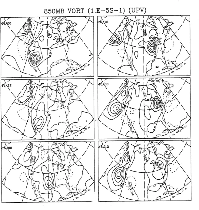
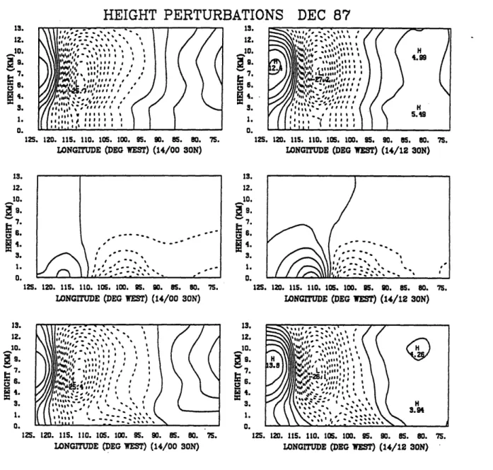
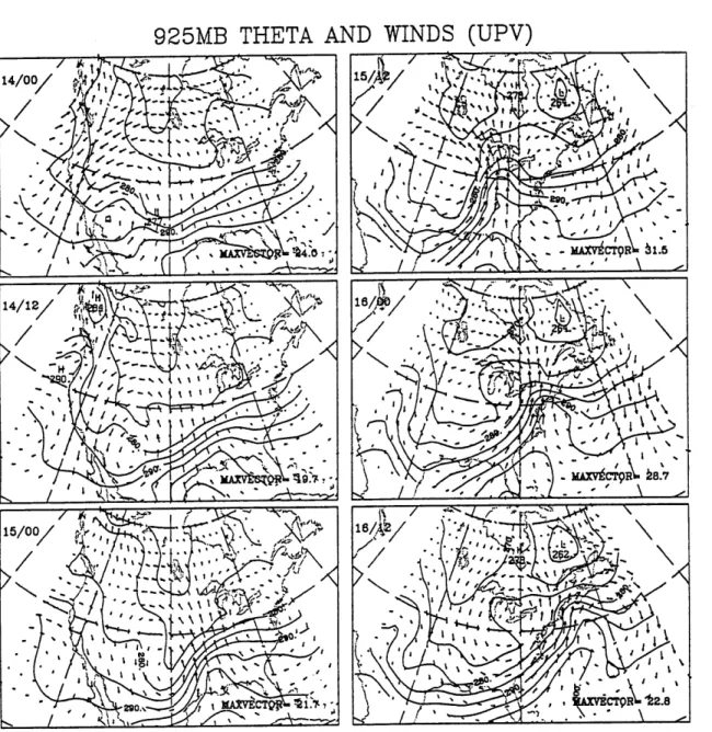
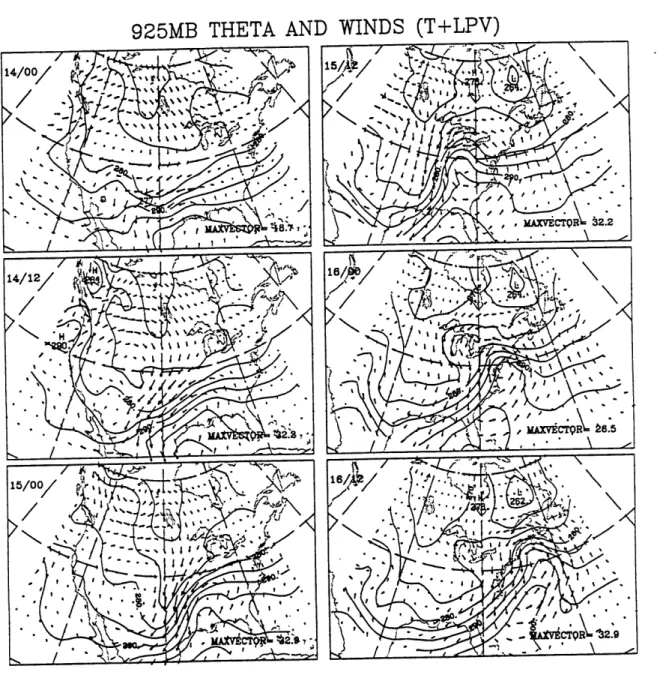
Chapter 3 Case I; December, 1987 64
Quantitative Contributions 68
Origin of Perturbations 74
Diabatic Effects 78
Summary 80
Figures 83
Chapter 4 Additional Cases 100
Case II; November, 1988 100
Figures 111
Case ///; February, 1988 122
Figures 132
Case IV; December, 1987(b) 144
Chapter 5 Summary and Discussion Summary of Cases Discussion Further Calculations Figures Appendix A References 165 165 170 176 181 186 188
Chapter A: Motivation, Objectives and Summary
Extratropical cyclones and anticyclones have been a prominent subject of research in meteorology for more than a century. The list of contributions from observational works alone is immense. Some of the more well known references are Bjerknes and Solberg
(1922), Petterssen et al. (1955), Petterssen et al. (1962), Palmen and Newton (1969), Petterssen and Smebye (1971), Sanders and Gyakum (1980), Bosart and Lin (1984), Uccellini et al. (1985), Boyle and Bosart (1986), Sanders (1986). In spite of all these, we believe a succinct view of the fundamental underlying dynamics of midlatitude developments from observations is generally lacking. The simplest way to understand the dynamics of a system is to diagnose its behavior in terms of conserved quantities which concisely embody the state of that system. However, the classical interpretation of observed cyclogenesis did not arise directly from the consideration of such quantities. In fact, the popular development scenarios described by Petterssen (1955) and Petterssen and Smebye (1971) were partly empirical results useful for forecasting rather than for describing the essential physics
behind cyclone intensification.
Beginning with Charney and Stern (1962), theoretical extensions of the classical studies by Charney (1947) and Eady (1949) began to focus on potential vorticity (PV) as the dynamic variable of fundamental importance in the study of midlatitude
cyclogenesis. Potential vorticity had been introduced some years before (Rossby 1940, Ertel 1942) as a scalar variable conserved following adiabatic, frictionless motion. The full usefulness of PV was realized with the knowledge that one could calculate the
motion itself given the interior potential vorticity, potential temperature on the boundaries and a prescribed "balance" relation
between the wind and temperature fields (Eliassen and
Kleinschmidt 1957; Hoskins, McIntyre and Robertson 1985, hereafter HMR). Through its properties of conservation and
invertibility, potential vorticity has come to be recognized as a
very important diagnostic tool for atmospheric motions on the synoptic and larger scales (HMR). Observational studies of cyclogenesis have not fully exploited the properties of PV to quantitatively diagnose developments in the real atmosphere. Because of this, there has been insufficient common ground on which to compare observed cases of cyclogenesis with the solutions of idealized theoretical and numerical models.
The properties of PV allow one to isolate the disturbances in the flow that are crucial to development from those that are incidental. This is necessary if one is to reduce the inherent complexity of typical atmospheric states to a level where the underlying dynamics becomes apparent. In this thesis, we will use the invertibility and conservation properties of PV to quantify the roles of the potential vorticity features most influential in the development process. Importance here is measured by the strength of the circulation associated with a particular feature and the
ability of that flow to amplify perturbations elsewhere. These calculations will form the basis for interpreting the observations
in terms of simpler models of cyclogenesis.
Specific questions we will address include (a) whether the significant interior PV features are concentrated at the tropopause, the steering level or distributed throughout the troposphere and what the importance of surface potential temperature perturbations is, (b) whether the development occurs with a vertical structure nearly constant in time or depends on a transient structure and, (c) what the influence of nonconservative processes (primarily latent heat release) is on cyclogenesis.
The first issue is related to the question of whether Eady "type" or Charney "type" dynamics are applicable. We use the word type here because we are referring to classes of behavior rather than specific models. In observed cyclone developments, we are unlikely to see either of these solutions in their pure form, hence we must look for potential vorticity distributions that signify different dynamical behavior. In a Charney type development, the significant PV perturbations are concentrated at the steering level and critical layer dynamics are important. The Eady scenario features no interior potential vorticity perturbations; the significant features are potential temperature waves at the upper boundary (or the tropopause) and at the ground. Synopticians have long pointed to the importance of waves in the upper troposphere in development (Bjerknes 1954, Petterssen 1955, Sanders 1986,
importance of tropopause perturbations. However, there are no calculations which cleanly isolate the importance of such waves in observed cases of cyclogenesis.
The second problem is related to the relative importance of modal versus non-modal growth in the atmosphere. Farrell (1984,
1989) has suggested that the transient development of
perturbations with an initially favorable vertical tilt against the shear may be of greater importance than growth due to modal instability. This type of development exhibits algebraic rather than exponential growth, but may intensify rapidly for a short time, perhaps enough to render an exponential growth phase
irrelevant. Although many descriptions of atmospheric
development suggest transient structures are prevalent (e.g. the above works concerning upper level waves), this issue if far from settled. Even a modal development will enter a nonlinear phase when the structure changes markedly after the low level circulation has spun up (Simmons and Hoskins, 1978). Hence, one must note the phase behavior during the most rapid stage of development. In most atmospheric observational studies, vorticity
at mid levels and at the surface are used to diagnose structural changes. Since stretching of vortex tubes provides a source of vorticity above a developing cyclone, the structure may appear more transient than when viewed from a potential vorticity perspective.
A third major issue investigated in this thesis is the importance on development of diabatic processes. Observational
studies have generally focussed on the effect of the latent heat released during the condensation of water vapor (Manabe 1956, Danard 1964, Tracton 1973, Bosart 1981, Dimego and Bosart 1982, Gyakum 1983, Emanuel 1988). Condensation is ubiquitous in nearly all mid latitude developments but its overall influence on cyclogenesis is still not well understood. Gradients of diabatic heating from condensation can act as a major source of PV in the lower troposphere. Thus, if we are able to identify that part of the PV distribution created by latent heat release, we can use the property of invertibility to calculate its contribution to the flow.
To investigate these issues, we examine four observed cases of cyclogenesis. Our procedure, which Chapter 2 outlines in detail, consists of breaking up the total potential vorticity distribution into pieces which have individual dynamical significance. We then calculate the flow associated with each of these perturbations and determine how each one contributes to the cyclone circulation directly or how it acts to amplify other features.
Our main results may be summarized as follows. For each case, we find that the low level circulation in the early stages of development is almost exclusively associated with potential temperature perturbations at the lower boundary. The low level winds from potential vorticity features in the upper troposphere contribute most to the amplification of the lower thermal wave. We also find that potential vorticity features in the lower troposphere likely result from the condensation of water vapor in stably stratified ascent regions. By this we mean that stratiform
precipitation, rather than convection, is the dominant type in the region of PV generation near the low level anomaly. These potential vorticity features are nearly colocated with the warm temperature phase of the low level thermal wave and, in two cases, contribute about 1/3 of the total low level circulation. Two of the developments feature initally large amplitude potential vorticity perturbations aloft and growth is transient. The other two cases begin with smaller upper tropospheric waves which grow during the low level intensification. These cases exhibit a relatively fixed phase structure during most of the cyclogenesis.
Because of the prominence of the interaction between
perturbations at the tropopause and at the lower boundary in each of the four cases, "Eady dynamics", modified by condensation in a way envisaged by Emanuel et al. (1987) and Montgomery and Farrell (1990) is deemed a roughly consistent paradigm for these developments.
Chapter 1 contains more background material, especially concerning potential vorticity and discusses some of the basic PV structures obtained from theoretical and numerical models of cyclogenesis. The application of some of our diagnostics to these quasigeostrophic solutions is also presented. The diagnostics appropriate for Ertel's potential vorticity are developed and discussed in chapter 2. In chapters 3 and 4, we present the four cases examined, each diagnosed using Ertel's potential vorticity. Chapter 3 reviews case I, which is fairly representative of the classic Petterssen development scenario. The three cases in
Chapter 4 serve mainly to contrast with this first case, and try to isolate those features that are common to each of the four developments. The first two cases feature somewhat smaller amplitude features in the initial state than case I. The last case in Chapter 4 serves two purposes. First, it presents a "null case" in which initial conditions were similar to those in case I, but development did not occur, at least not in the same region. Cyclogenesis did occur later in time and this development forms the fourth event on which our results are based. These results are discussed in Chapter 5, in which we also suggest some additional diagnostics that might be illuminating.
Chapter 1: Background
The purpose of this chapter is to summarize the different diagnostics used in previous studies of developing extratropical
cyclones. The general progression we outline is from
semi-empirical approaches, partly rooted in weather forecasting, to the more quantitative diagnostics of the potential vorticity perspective. We then present the potential vorticity structure of solutions to the Charney and Eady problems of baroclinic instability and show the results our diagnostics yield when applied to these models. The distinctions between these simple models will provide a useful foundation for interpreting the observed cyclogenesis cases.
Vorticity and Divergence
The diagnosis of cyclone development from observations has generally focussed on the behavior of the low level wind circulation with time. The basic approach has often been to investigate related quantities such as vorticity (the vertical component of earth-relative vorticity) or perturbation pressure (the departure from an instantaneous background field) from which the low level winds can usually be inferred. To deduce changes in either low level vorticity or surface pressure, the essential quantity is the horizontal divergence of the flow.
sought to relate the vertically integrated mass divergence (which must be positive over a pressure minimum at the surface for deepening to occur) to particular configurations of waves at different heights in the troposphere. The importance of the
convergence-divergence patterns associated with waves in the upper troposphere soon became apparent. Bjerknes and Holmboe were able to deduce that divergence (convergence) aloft was likely downstream (upstream) of upper level troughs. This implied a preferential phase in the large scale wave pattern for surface pressure falls (downstream of troughs) and rises (downstream of ridges). They also inferred the importance of a westward tilt with height in an amplifying baroclinic system. Ten years later,
Bjerknes made a useful contribution to forecasting by identifying the qualitative shape of upper level troughs which most favored downstream divergence. These "diffluent" troughs simply had
stronger winds upshear than in the downshear direction.
Unfortunately, the utility of divergence as a diagnostic quantity is limited in practice. There is generally a near cancellation between divergence aloft and convergence at the surface (from inertial inflow and friction). Hence, the favorability for arbitrary perturbations to develop is determined by the small difference between two large terms. Further, divergence is itself the difference between two nearly cancelling derivatives of the wind field (au/ax = -av/ay), hence it is difficult to measure accurately from observations.
The diagnosis of vorticity changes also implies a need for the divergence since the vertical stretching of vortex tubes has long
been recognized as the major source of vorticity in cyclone scale systems For inviscid, synoptic scale motions, the vorticity equation may be approximated as
D(f + C)/Dt = -(f + C)8 where f is the Coriolis parameter, relative vorticity and 5 is the divergence need only be known Lagrangian vorticity change at that applied in its quasigeostrophic form divergence
(1.1)
r is the vertical component of horizontal divergence. Here,
at one level to estimate the level. Equation 1.1 is usually by neglecting r coupled to the (setting f=constant) and approximating the substantial derivative by the rate of change following the geostrophic flow. As an alternative to estimating divergence directly from winds, it can be calculated given the vertical motion field obtained from the 'o' (=Dp/Dt) equation (Holton p137)
f02 )pp + (yV20) = fO( Vo Vr )p + V2( V* Vo ) + Cp-1V 2(as). (1.2)
Here the gradient operator is two dimensional, the winds and vorticity are geostrophic, a=RT/p, a(p)=-aX(lne)p is the static
stability parameter, s=Cp Ine is the specific entropy, and friction has been neglected. The omega equation, together with appropriate boundary conditions forms an elliptic boundary value problem provided a>O and also completes the quasigeostrophic (QG) system of prognostic equations (vorticity, co and mass continuity). There are other ways to write the r.h.s. of (1.2), but this form of the co
"differential vorticity advection" (first r.h.s. term) and "thermal advection" (second term), (Petterssen 1955, Sanders 1971, Tsou et al. 1987). This distinction is rather arbitrary, however. That these terms tend to cancel was noted by Sutcliffe (1947) and Trenberth (1978), who both proposed the advection of absolute vorticity by the thermal wind as a useful approximation to the inhomogeneous terms.
The o equation has since been reformulated by Hoskins, Draghici and Davies (1978) who write the r.h.s. of (1.2) as twice the horizontal divergence of a vector Q. The advantages of the Q-vector formulation are that one can estimate the sign and relative magnitude of vertical motion (away from boundaries) from a single vector field. The Q-vector field turns out to be mostly divergent, hence VeQ is rather easily deduced in practice (Hoskins and Pedder, 1980).
Results of studies using the vorticity and omega equation diagnostics further supported the importance of ascent roughly 1/4 wavelength downstream of large amplitude positive vorticity features in the upper troposphere. Since these features were believed to exist prior to low level development, important variations in the low level structure were required which favored cyclogenesis only at certain times. Emprical findings by Petterssen et al. (1955) supported his proposed hypothesis that "cyclonic development at sea level commences when and where an area of positive vorticity advection in the upper troposphere becomes superimposed upon a frontal zone at sea level". Sanders (1971) offered some quantitative support of this by considering solutions
to the quasigeostrophic system for an idealized wavelike perturbation in the presence of vertical shear. His basic findings were:
(1) Intensification of the sea level system is associated with a low level divergence field partly in phase with the surface pressure perturbations. The stretching of vortex tubes is in turn related to vertical motion required to preserve thermal wind balance in the presence of vorticity advection increasing with height. This effect arises from the shear and westward tilt with height imposed on the perturbation in his study. The growth rate of the disturbance is found to be nearly linearly proportional to the shear.
(2) The translational velocity of the 1000mb geopotential perturbation is determined primarily by low level temperature advection (and is maximized for a warm core surface low).
(3) The maximum growth rate for a given vertical shear occurs for disturbances with wavelengths between 1500 and 3000 km.
This analysis qualitatively reproduced the results of the theoretical calculations performed earlier by Charney and Eady which we discuss later in this chapter. However, the form of the perturbations was assumed a priori on the basis of qualitative resemblance to observed systems.
Over time, a popular view arose that there existed two basic types of development which Pettersen and Smebye (PS hereafter) tried to define in their 1971 paper. They based the character of two prototypes of cyclogenesis on differences in the vorticity evolution at upper levels and the strength of the low level
baroclinicity. In summary, type 'A' cyclones were frontal waves having initially large amplitude at low levels compared to aloft, similar to the classical solutions obtained by Charney. Amplification at upper levels occurred later, but was viewed as a by-product of the low level development rather than an instigator.
Type 'B' developments depended on the existence of an intense upper level feature prior to surface cyclogenesis. One gets the impression that this type of development is intended to be analogous to that described by Petterssen (1955). However, PS are very unclear concerning the importance of surface baroclinicity. Low level fronts may be present in their type 'B' scenario, but PS stress the smallness of low level temperature gradients, which seems contradictory.
There are other weaknesses in the classification scheme proposed. First, for type 'A', it is not mentioned how one distinguishes between upper level wave amplification associated with the low level cyclogenesis (Sutcliffe's "self development") and growth related to other processes (local interference effects, for instance). Second, there is no clear dynamical basis for separating developments on the basis of dominance of either "vorticity advection" or "thermal advection" (Trenberth, 1978).
Boyle and Bosart (1986) present a case where there is a large amplitude pre-existing upper wave, but the diagnosed vertical motion is associated almost equally with both vorticity and themal advection throughout the development. Finally, there may be other characteristics which would make this class separation of cyclogenesis more meaningful. Such quantities as phase speed,
precipitation (where it occurs relative to the cyclone and the overall influence of latent heat released in condensation) and the decay process may vary significantly depending on whether or not the amplitude aloft is initially large.
The effect of latent heat release on cyclones has also been investigated using the vorticity and o equations (e.g., Danard 1964, Tracton 1973, Tsou et al. 1987, Gyakum and Barker 1989). For ascent in saturated, stably stratified regions (with respect to a moist adiabat), the diabatic heating may be taken proportional to c
(Haltiner and Williams, 1980). This allows the heating to be incorporated into the I.h.s. of 1.2 by introducing a modified static stability parameter, am, reflecting the moist stability. A
disadvantage of the co equation consistent with QG is that no horizontal variation of am is allowed, hence this amounts to
reducing the stability everywhere. By not making the QG
approximation, the up-down asymmetry may be included (see chapter 2).
In general, however, neither the "continuity" nor the "vorticity-co" approach is very adept at isolating the features of the flow that are crucial to development. In addition, because vorticity has an important source in adiabatic motion, it has limited use for diagnosing the effects of condensation on cyclogenesis. Given the amount of "noise" and clutter that may be seen by even a casual glance at weather charts, one needs a way of distinguishing features and processes crucial to development in a dynamically meaningful way. This is important if we are to
compare observations to the idealized environments of theory and models of cyclogenesis. The following section describes the use of potential vorticity as a diagnostic tool for this purpose.
Potential Vorticity Diagnostics
Although potential vorticity has been used to diagnose atmospheric motions for some 50 years now, extensive application of its dynamical properties in observational work has only been made within the last decade (see HMR for a thorough review). Ertel's potential vorticity and its prognostic equation (Ertel, 1942) are defined by
q = p-1 j * V
e
(1.3a)Dq/Dt = p-1 (*11 V Q + VO * V x F) (1.3b)
where p is the density, 1 is the three dimensional vorticity vector,
Q=DO/Dt and F is the frictional force. Hence, assuming adiabatic, frictionless motion, q is conserved following the flow.
Examination of potential vorticity in the upper troposphere and lower stratosphere (Eliassen and Kleinscmidt 1957, Bleck and Mattocks 1984 and HMR) has helped clarify the identity of the mobile upper waves often involved in cyclogenesis (Sanders 1986, 1987). These can be viewed as undulations in the tropopause, where we consider the tropopause as a surface of constant PV located in the sharp transition region between tropospheric and
stratospheric air (Danielsen, 1968). Maps of PV are often displayed on isentropic surfaces. When the r.h.s. of 1.3b vanishes, PV is conserved following the "horizontal" wind in this coordinate system. If the hydrostatic approximation is valid, this is the
almost exactly the horizontal wind in geometric coordinates. Also, in q coordinates, the formula for PV reduces to
q = -g (ap/a)-I( f + ) (1.4)
where oe refers to the the vertical component of vorticity computed on an isentropic surface. On such surfaces, troughs (ridges) correspond to deflections of the tropopause toward lower (higher) ambient values of PV. The height of the tropopause also varies with these disturbances, being depressed (elevated) in troughs (ridges). As shown by Thorpe, 1986, the difference in tropopause height between realistic positive and negative PV perturbations may exceed 5km.
In addition to its quasi-conservative properties, potential vorticity also determines the flow by which it is advected, hence PV a dynamically active "tracer" of air motions. The work by HMR emphasizes that given the PV distribution and certain constraints, one can calculate a unique flow associated with it. This is known as the invertibility principle. One constraint is that the calculated flow must adhere to a prescribed relation between the wind and mass fields, an example being the thermal wind equation. This constraint, known as a "balance condition", allows one to set up a
mathematical boundary value problem that relates q to the flow. A second constraint is that boundary conditions must be specified.
In general, this means specifying the distribution of 0 on the horizontal boundaries and some component of balanced wind on the lateral boundaries. If the domain is laterally infinite and not periodic, a reference state must be specified. Third, existence of a well posed problem requires the system to be elliptic. For inversions of Ertel's PV, this necessitates f.q > 0, a condition which eliminates buoyant convection and symmetric or inertial instability. Therefore, by our definition, these types of motions
cannot be considered as part of the "balanced" flow. The
usefulness of the invertibility property of PV depends on the
accuracy of the mathematical balance relation imposed.
As an application of invertibility, consider pseudo-potential vorticity (Charney and Stern 1962). Equation (1.1) may be combined with the QG thermodynamic equation to obtain a conservation statement for a scalar following the geostrophic flow
(in z coordinates)
D9q = Dg{ V2V + 3(y-yo) + f
02p-l(pN-2Vz)z } = 0 (1.5)
Here y is the geostrophic stream function (N=/fo), Dg is the substantial derivative following the geostrophic motion, p=p(z) is
the density, N2-N 2(z) the Brunt Vaisala frequency and 3=df/dy
evaluated at y=yo. The expression is valid in the absence of vertical gradients of diabatic heating and when the curl of the
frictional force has no vertical component. The complete system needs boundary conditions. Assuming a flat lower boundary, we have conservation of potential temperature Dg(Vz)=0, (z=zo). At
the top either a rigid lid is imposed, in which case the upper and lower boundary conditions are the same, or boundedness of the solution is required as z-=o. In many theoretical applications, the domain is periodic in x and bounded in y. The perturbation flow is
usually forced to vanish on the north and south walls.
This system consists of a conserved quantity q related to the balanced (geostrophic) flow by an elliptic operator (for N2> 0). The
basic scaling assumption which leads to this conservation relation is that the spatial and temporal Rossby numbers U/foL and 1/foT must be small compared to unity. Here, U is a characteristic variation of the flow, L is a characteristic length scale over which it varies and T is a time scale for the motion. The balance condition is a trivial algebraic expression y=~/fo. In principle, given any arbitrary initial distribution of q, one can invert it to find the V field, advect the q field, invert again and so on. An important point is that the definition of q is a linear equation for
V, hence we may invert any ensemble of q anomalies individually and then add them up to recover the total flow. The strength of a given q anomaly is thus measured by the strength of the balanced flow associated with it. This approach is especially useful in assessing the interaction of isolated anomalies (as in a problem with many point vortices). An example is the qualitative argument for Rossby wave propagation (Pedlosky 1979, p102 and HMR) which
utilizes the invertibility principle and the conservation of q. In addition, Bretherton (1966a) showed that the distribution of e on the lower boundary (0B) is equivalent to a 8-function contribution
to the interior PV just above the ground. This mathematical device allows one to think of the lower boundary 0 field as part of the total potential vorticity distribution.
As previous observational work has suggested, there are likely only a few distinct PV features associated with most cases of cyclogenesis. It is therefore not our goal to dissect the flow ad
infinitum, but rather to identify coherent PV distributions and assess their relative contributions to development using the concepts of invertibility and PV conservation.
We have already mentioned the upper tropospheric waves that synopticians have long associated with cyclogenesis. Other authors (Manabe 1956, Uccelini et al. 1985, Boyle and Bosart 1986, Hoskins and Berrisford 1988) have mentioned the presence of low level PV perturbations near the warm front in cyclones. All of these authors cite latent heat release as the most likely source of this low level PV. Hoskins and Berrisford (Hoskins, personal communication) have tried to estimate the contribution of such a
low level anomaly of Ertel's PV found in the Eastern Atlantic storm of October, 1987, using a two dimensional semi-geostrophic inversion technique. They find the low level winds enhanced by nearly 20 ms-1 by this feature. There are also perturbations of e
g
which can be quite pronounced in cyclones. Although Hoskins and Berrisford find such features unimportant in the mature structure
of their case, Thorpe (1986) has shown that a realistic boundary anomaly of potential temperature can be associated with vorticity of order the Coriolis parameter.
Potential Vorticity in Simple Models
In the reconciliation of observations with the theoretical solutions for developing disturbances, PV concepts can also be of
use, since most of the of the simple models of cyclogenesis yield perturbations with very distinctive PV structures (although the pressure fields may have many similarities). Of course, many variations on the original works of Charney (1947) and Eady (1949) have been studied. For simplicity, we shall consider only the classical structures in those two works as prototypes for developments involving critical layer and tropopause PV anomalies respectively.
Robinson (1989) has performed a study in which he calculates the flux of PV (and surface 0) at various levels using velocities obtained by inverting PV at other levels as well as surface 0. However, it is not clear how far this approach goes toward "explaining" baroclinic instability by addressing the issue of causality (Lindzen, 1988). It seems to give more insight into transient developments of the type discussed by Farrell (1984, 1989) or in assessing what would happen if the structure of a mode were suddenly perturbed. In dealing with modal solutions (or "phase locked" growth in the real atmosphere) we will simply try to identify consistency with certain theoretical solutions.
With the above discussion in mind we present an analysis of the Charney mode (k=2, 1=1.47, N=0.012 s-1 and r=1.5 from Snyder and Lindzen 1988) and the Eady mode (k=2, 1=1.47 and S = (NH/fL)2 =
0.5 from Pedlosky 1979). These are designed to indicate a possible range of structures we may encounter. Figures 1.1(a) and (b) show the perturbation 0 and geopotential respectively, while in (c) and
(d) we have calculated 0' associated with the temperature perturbation at the top (c) and at the bottom (d) boundaries. We note the familiar eastward tilt with height of the thermal field and the larger westward tilt with height of the geopotential (roughly n/2 bottom to top). There is no variation of interior PV in the Eady model, hence (c) and (d) sum to the total perturbation. We see the phase shift between these two anomalies is roughly 0.4 wavelengths with warm temperatures on the lower boundary corresponding to negative 0' and the opposite on top. One qualitative interpretation (Bretherton 1966b, and HMR) is of counterpropagating Rossby waves at each boundary which are deep enough to "lock on" to each other. This means that there is an
upshear phase shift between the lower and upper waves that allows the circulation from one to amplify the other and slow the other's propagation enough to keep the structure fixed. The downgradient heat flux at one boundary is, in fact, completely due to the presence of the 0 anomaly at the opposite boundary.
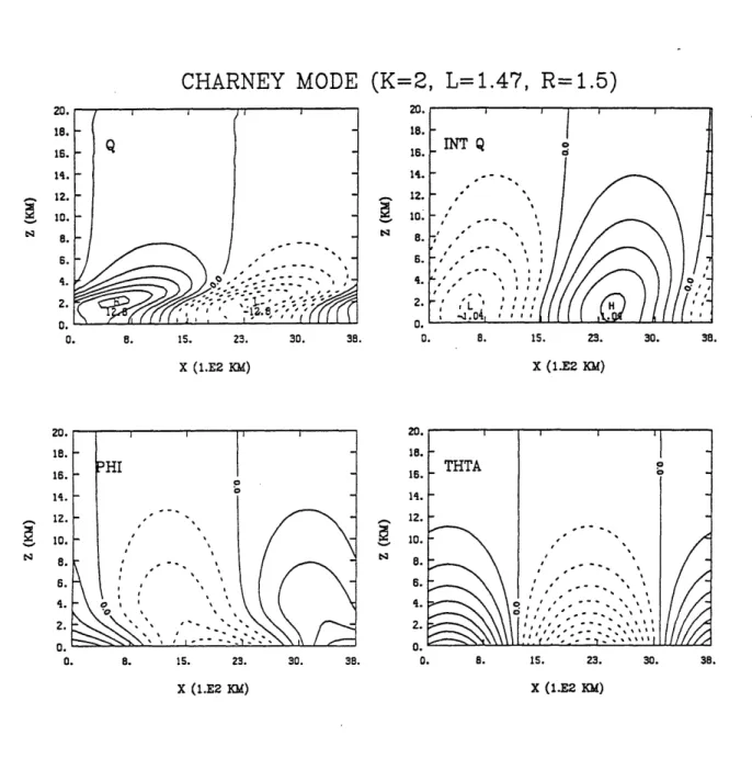
The Charney mode has its own characteristic signature which is shown in figure 1.2. There are significant PV perturbations in the interior concentrated at the steering level and thermal anomalies at the lower boundary (the calculation was performed
with a lid at 4 scale heights, but thermal anomalies there are
insignificant). A phase relationship very similar to the upper and
lower Eady perturbations exists here between the PV at the steering level (2 km) and
e
at the ground, but the interior PV has a significant phase structure of its own. HMR go through a similar kinematic arguement for this structure as well. For purposes of identifying such a structure it is sufficient to know that the main PV is at the steering level, the geopotential anomaly associated with it is comparable in strength to that of the eB field and thephase lag between the two is about 0.4 wavelengths.
For baroclinic growth of non-modal form, there are an infinite number of properly configured initial perturbations that will grow transiently. Farrell (1989) has removed much of this arbitrariness
by seeking the initial structure that grows maximally for a given
basic state in a given time, provided one specifies what norm is used to measure the amplitude. It is unfortunate that the richness of these "optimal" initial structures is not likely amenable to observational identification as Farrell points out. It is also not clear why the atmosphere should select an initial state that is
optimal for growth. However, his works have emphasized the possible robustness of transient developments. The degree to which the vertical structure of the PV changes during development can be useful for determining the relative roles of transience and
phase locked growth in a given cyclogenesis event.
The addition of latent heat released in the condensation of water vapor can significantly alter the structures described above.
For instance, Emanuel et al. (1987) parameterize the effect of the condensation as reducing the effective static stability to near zero in the ascent region of an Eady model. In semigeostrophic theory, this means that the moist Ertel's PV (qe) becomes very small
where air is rising and assumed saturated. A PV conservation law applies here as well, provided we define the PV in this region using
Oe as the thermodynamic variable
0e = 0 exp( Lvw/CpT ) (1.6)
where Lv is the latent heat of condensation (assumed constant), Cp
is the specific heat of air at constant pressure, w is the (saturation) mixing ratio and we have ignored the effects of water vapor on the heat capacity. In fact, in a saturated atmosphere with no liquid water, qe with Oe on the boundaries specifies the
invertibility problem for the flow (Emanuel et al.). Conservation even in the presence of gradients of diabatic heating offers a conceptual advantage over viewing the problem in terms of dry PV, for which sources and sinks would exist. However, such a state of continued saturation over an entire baroclinic wave is a rather contrived situation. Since the atmosphere is only locally saturated, different forms of PV in the saturated and unsaturated regions would be needed to have conserved quantities both places. Then one would have an internal boundary at the saturation interface along which 0 or 0e would have to be specified. This
would hardly simplify the problem because the boundary would be free to move in the real atmosphere and take on very contorted
shapes.
As it turns out, the vertical derivative of the heating generally dominates the generation of dry PV, being positive below the heating maximum and negative above (eq 1.3b). As shown by Emanuel et al., the positive PV generation maximizes at the ground underneath the narrow ascent region. This updraft actually collapses to a sloping sheet in the limit qe-0. Because the flow in the generation region is less than the wave speed, the high PV extends in the upshear direction with time (in the wave's frame of
reference). The absence of diabatic heating (and friction) at the boundaries implies that the mass weighted integrated PV in the domain must remain constant (Haynes and McIntyre, 1987). The low level generation is compensated in this integral sense by destruction of PV aloft. The negative anomaly aloft is much more spread out however and is partly advected downstream by the shear
flow. Both the analytical and numerical results presented in this paper reveal increased growth rates in the moist waves of about a factor of two relative to the dry waves, with no change in the phase speed.
The effects of latent heat release have also been incorporated into the Charney problem as a Wave-CISK model of cumulus heating (Snyder, 1989). The addition of such heating in the Charney problem does not always lead to enhanced growth with respect to the corresponding dry modes. The effect of such heating seems to involve the relation of its vertical structure relative to the profile of u(z)-cr (at least for small growth rates and weak heating that
obeys certain thermodynamic constraints). When PV generation occurs at the critical level, it tends to cancel the critical level PV of the dry mode and stabilize the perturbation. If the generation
region is above the critical level, there is little effect of the heating; this is a regime applicable to short wavelengths. Finally if the heating maximum coincides with the critical level, there is
less opportunity for cancellation and enhanced growth is possible.
In general for realistic heating parameters, the most
destabilization occurs when the shear is large and the heating confined to low levels.
Potential vorticity has other sources and sinks from such processes as radiation, evaporation of water and turbulent mixing.
In this thesis, we will not explicitly consider the influence of these processes on cyclogenesis. The importance of evaporation in cyclones is largely unknown, perhaps because of its complexity and the difficulty of obtaining reasonable evaporation rates from data. Radiation in the troposphere has a time scale compatible with cyclogenesis only near the ground. The effect of heating (cooling) at the ground on the pressure field is nearly cancelled by the destruction (creation) of potential vorticity just above the surface. Turbulent mixing in the boundary layer complicates this picture, however. In addition, turbulence occurs in the free atmosphere and can act as a source of PV on the scale of observations, especially near the tropopause (Shapiro, 1976). Limitations of the data we use rather than the unimportance of these processes will be the primary reason for their neglect.
EADY MODE (K=2, L=1.47) TI' k /j ois-, s I I ## I II # a ll isl" 66, , ,, :, 6. !ie r e rt , -I (d I I I -r,, 6, l - ,, r l I il l at 0. i . 23. 30. 38. 0. X (1.E2 1KM) s o I 1 %10. % % r ' _ , I , ,, , 9.0 ., 6 i6O 7. •I \ v ~5. N . ,3. X ( K 0. 8. 15. 23. 30. 38. 0. x (1 .E2 M) 8. 15. 23. 30. 38. x (1.E2 KM) , is so I I .6 I 6 0 /I ..~ ~ , -" lI e # l o , --a 6 : " 11 It 11 ! 1 # I 1l I 23 30 # 38 X (1.E2 KU) 6 6 6 t I I ! ( ## " I ! 1 ! ( # s , ti I I ! i o # \ ( I I I o / I t ' i ( I i I
\\III"
66 6...
6 0666, 0 ' 6 6666 l i r , 8. 15. 23. 30. 38. x (1E2 1CM)Figure 1.1 Eady mode fields; (a) potential temperature (b) geopotential perturbation
(c) geopotential perturbation associated with only the upper boundary temperature
perturbation and (d) geopotential associated with the lower boundary thermal field.
All fields are nondimensional (linear mode amplitude is arbitrary). Contour interval
for all geopotential fields is 0.2
10. 9. B. 7. 6. 5. 4. 3. 2. 1. 0. 0.
CHARNEY MODE (K=2, L=1.47, R=1.5) 20. 18.-14. -S 12. -," - 10. ," 8. i- . 15. 23 .3-9. 3L 2. , . ,15 30. 38. 8. X (1.E2 KoM) 20. 18. 16. 14. S12. - 10. S- " 8. -- . S . 0. 2 4. 2.
S0.
8. 15. 23. 30. 38. 0. 8. 15. 23. 30. 38. X (1.E2 KM) X (1.E2 KM)Figure 1.2 As in figure 1.1, except for Charney mode and (a) shows PV rather than
potential temperature. 20. 18. 16. 14. 12. 10. 8. 6. 4. 2. 0. 0. 20. 18. 16. 14. 12. 10. 8. 6. 4. 2. 0. 0. x (1.2 KM)
Chapter 2: Diagnostics
Here we present further details of the diagnostics to be used
in this study. Having discussed quasigeostrophic pseudo-PV in Chapter 1, we concentrate here on developing a technique for calculating and inverting Ertel's potential vorticity. The salient feature of the diagnostic framework we develop is that we require only the potential vorticity, relative humidity and boundary conditions as input parameters.
Data and Computation of PV
An obvious disadvantage of PV is that is cannot be measured directly but rather must be calculated from the wind, temperature and pressure fields. The data we will use to do this consists of the gridded final analyses from the National Meteorological Center (NMC) (see Trenberth and Olsen, 1987 for an overview of the data
and assessment of qualtity). The format is a global
latitude-longitude grid with 2.50 spacing in both horizontal directions and 10 levels in the vertical (1000, 850, 700, 500, 400, 300, 250, 200, 150, and 100mb). The fields we will use at these levels are wind, temperature, geopotential height and relative humidity (up to 300mb) along with pressure and temperature at the earth's surface, all analyzed twice daily at 00 and 12 GMT. The initial guess for these fields consists of the 12 hour forecast of
the NMC Global Spectral Model; the primary data source is the conventional upper air and surface network, with supplementary data supplied by aircraft and some satellite information. The analysis performed on the wind and temperature is "multivariate optimum interpolation" (Lorenc 1981), but the data have not undergone a formal initialization procedure.
In this study, we will restrict our attention to cyclones over North America, which affords us the opportunity of examining the raw soundings and the surface hourly and synoptic reports on which the NMC analysis is based. Using the GEMPAK analysis package we can also perform objective analyses (single parameter Barnes' scheme) to check the PV calculated from the NMC data.
The basic calculation of potential vorticity will be done by expanding the dot product in 1.3a into three terms (ignoring the components of vorticity involving vertical velocity)
q = -g]Tp-1 ( TIOe - (a.coso)-lv,e + a-'u,,O ). (2.1)
Here, n(p)=Cp (p/po)" is the Exner function, x=R/Cp, a is the earth's radius, X is the longitude, p the co-latitude and subscripts denote partial differentiation with respect to the subscript variable. We introduce the Exner function vertical coordinate because of the simplicity of the resulting hydrostatic relation (appears in a Boussinesq form). Spherical coordinates are introduced for convenience in performing calculations from latitude-longitude based data and to allow the full variation of the Coriolis parameter. From 2.1 we obtain the PV at 8 levels in the vertical
from 850 to 150mb by using centered finite differences to estimate derivatives. Appendix A provides a crude estimate of the expected error in PV from random wind and temperature errors. For this data, errors range from 0.2 PVU at low levels to 1.2 PVU in the lower stratosphere where 1 PVU = 1 m2 K kg-1 s-1 (HMR). There
is a tendency for random errors in PV over one grid volume to be cancelled out in adjacent volumes. Hence, the balanced flow, being an integral over the PV, may be relatively uneffected by small scale noise.
Given that 2.1 contains only first derivatives of observed quantities, it would have been better perhaps to stagger the grid in the vertical. The problem with this occurs at the lower boundary where we must specify the potential temperature in the invertibility problem. The 1000mb level is generally below the earth's surface in our domain and the field of 1000mb temperature in the NMC data is largely extrapolated downward given the surface temperature and low level static stability. This produces 1000mb temperatures that are not hydrostatically consistent with the height field. The reason is that the 1000mb geopotential field is calculated by integrating the hydrostatic relation downward from the surface using a standard atmosphere profile of temperature which may depart significantly from the profile just above the
ground. In our calculations we will use the mean potential temperature in the layer between 850 and 1000mb as our lower boundary condition for inverting the PV. Consistent with this, we use the height field to estimate the static stability at 850mb (and
at 700mb over high terrain where 850mb is below ground). We use the analyzed winds at all levels, even where they have been extrapolated below ground.
To obtain the upper boundary condition, we integrate the static stability upward from our lower boundary 0 at 925mb up to 125mb. We are, in effect, specifying the mean static stability in our domain by imposing 0 at the top and bottom boundaries. If this is not consistent with the mean stability used in the computation of PV, there can be a bias in the domain integrated absolute vorticity.
Of course, if the complications at the lower boundary did not exist,
we could use temperatures at all levels and stagger the PV grid which would guarantee consistency between the mean stability and
o
at the two boundaries.Inversion of PV
In chapter II, we presented the inversion problem for quasigeostrophic pseudo-potential vorticity in terms of an elliptic boundary problem for the geostrophic flow given PV and 0 on the boundaries. This pseudo-PV is conserved following the horizontal geostrophic flow with errors being O(Ro). On the other hand, Ertel's
potential vorticity obeys an unapproximated conservation relation in the absence of diabatic and frictional effects. Charney and Stern (1962) showed that as long as the Rossby number is small, the variation of pseudo-PV on a pressure surface is proportional to the variation of Ertel's PV on an isentropic surface. As pointed out
in HMR however, there are recurring situations where the variation of the two is not approximately the same. One is in frontal zones, where the slopes of the isobaric and isentropic surfaces may substantially depart from each other. Another is near the tropopause, where horizontal variations in the static stability can be first order effects. In addition the geostrophic balance assumption may suffer quantitative inaccuracies in regions of strong flow curvature. Hence, for studying real atmospheric flows,
it would be useful to have an invertibility relation for Ertel's potential vorticity that is accurate in situations of large flow
curvature.
The equations we develop for this purpose are based on the systematic neglect of the irrotational part of the flow compared to the nondivergent part. The balance condition we will use was first formulated by Charney (1955) and is also derived in Haltiner and
Williams (1980). The procedure begins by decomposing the horizontal wind field into nondivergent and irrotational parts (denoted v and vz respectively). In an unbounded or periodic
domain, Helmholtz' Theorem states that such a partitioning is unique. However, as pointed out recently by Lynch (1989), in a bounded domain there can be a contribution from the harmonic field
(no curl or divergence) such that v, + vZ * v. In realistic cases in a
bounded domain, however, we shall show that the momentum of the harmonic field is quite small compared to the other two parts of the velocity field.
The Charney Balance Equation is obtained by operating with the horizontal divergence on the momentum equation and performing a scaling analysis in which terms proportional to vZ and vertical
velocity are neglected compared to those proportional to v,. For
the nondivergent flow we then define a stream function
u = - a1 X v
V = (a-cosO)-Yx (2.2)
such that r = V2y is the full vorticity (with the Laplacian in
spherical coordinates). The resulting balance condition may be written
V20I = V2I + Vf * V' + 2-(a.cosO)-2{{ T - (y1*i)2 } (2.3a)
where V is the horizontal gradient operator. A similar scaling
analysis may be used on the definition of PV (2.1) to relate q to the geopotential 0 and the streamfunction T,
q = gip-1 { (f + V2T)(D, - (a.cosO)-2( ), ) - a-2( )
}.
(2.3b)
This equation combined with the Balance Equation forms a system of two coupled nonlinear equations. We shall refer to this as the Balance Equation System (BES) to distinguish it from 2.3a alone.
A system very similar to the BES was investigated by Charney
(1962) and found to be elliptic for q > 0. We note that the condition
for ellipticity of the Charney Balance Equation by itself as a problem for T given 0 is approximately V24 + f2/2 > 0 (Courant and
Hilbert 1962). This condition is frequently not satisfied in the atmosphere (Iversen and Nordeng 1982) whereas q > 0 is a less stringent requirement that is generally observed to hold. Even so, the PV calculated from data can be negative locally, in which case, there will be no solution to the boundary value problem we wish to pose. We therefore will set negative values of PV equal to a small positive constant well within the uncertainty of the calculated values. Support for this approach is that we have observed PV to become negative in data sparse regions more frequently than in data rich regions.
To complete the problem, we must specify boundary conditions. At the upper and lower boundaries we specify 0 and the condition
on 0 is just the hydrostatic equation
ON = - 0 ( x = xo and x = xt ) (2.3c)
Equation 2.3b also requires a condition on Y at the upper and lower surfaces. We adopt a geostrophic condition, namely
Y, = - O/fo ( x = no and n = nst ) (2.3d)
A more consistent relation might be derived from the vertical
derivative of the Balance Equation, but we have found the interior solution is very insensitive to the condition imposed on ' since the term containing the boundary information is generally small (but kept for consistency). Indeed, the last two terms in 2.1 can be eliminated by a transformation to isentropic coordinates.
On lateral boundaries, we require the geopotential to match its analyzed value. The streamfunction is also specified on the lateral boundaries by integrating
S Sf v *ndl
s
= v n - dl (2.3e)
JC
around the edge where 'C' is a closed path around the edge of the
domain, n is the outward facing normal and 's' implies a direction
along the edge moving counterclockwise (parallel to I). Because there can be a net divergence of the observed wind over the domain, the integral of the normal velocity around the edge need not vanish. The second term on the right hand side of 2.3e subtracts off the net divergence so that T is continuous everywhere along the edge. The constant of integration in 2.3e is supplied by setting = D at one point on the boundary (a similar condition was used by Iversen and Nordeng, 1982).
Method of Solution
Because the BES is coupled and nonlinear, solution even by numerical methods is not straightforward. The technique we describe below was developed largely through experimentation; however, it appears to be quite general in its ability to converge to a solution.
The complexity of the equations led us to consider an iterative method of solution, namely a modified form of successive over relaxation (SOR). To describe this procedure, we need to refer to
denote the discrete values of the streamfunction and geopotential respectively. In general, three subscripts are needed to specify a gridpoint, however, we will only use subcripts to denote locations relative to a particular point. For example, 'ij-l,k will simply be S.j-. In what follows, subscripts i,j and k denote latitude, longitude and x(p) respectively. With this notation, the finite difference forms of 2.3a and 2.3b are
V2I = fV2T + ( -fCOSV)(Vi2 -Pi+ )/y + (2co0S-2).( Ax-2.A-2 ).
{ ('j+l+j..-2W)( +i+1+Ti-1-2T) - A ) (2.4a)
and
q = gKicp-l{ (f + V2 y)( (Dk+1-0)/Ax+- (D-(k-1)/An- )/x -O
}
(2.4b) where
A = (Yi- ,j+l-P i+l,j+- i-l,j l+ i+l ,j-1)2/1
6
E = (A-2).[ (Ax-2Cos-2 )(Pj+ ,k+l- j-lj,k+l-j+l,k-l+ Yj-1,k-1) ((Dj+1,k+1- j- 1,k+1 - j+l,k-1 + j-.1,k-1)/16
-(Ay-2)(1y i-1,k+1 i+1,k+1" i-1,k-1+y'i+1,k-1) '
(Di-1,k+1f- i+l,k+1 -'i-l,k-1+( i+1,k-1)/16 ]
and we have introduced the symbols
V2(A)= cos-20 { (Aj+
1+ Aj. -2A)/A x+ coso ( (Ai.l-A)cosi-1/2
Ay= a-A ; Ax= a-A ; A,= (Xk+1-/k-1)/2 ; Ax+= (I7k+1- ) ;
Our iteration begins with an initial geopotential field taken from the analysis, and initial stream function obtained by solving
V2T = C, the observed relative vorticity, at each level. The iteration process we describe is nested, hence it requires two iteration indices. The superscript o will be the "major" iteration index, and v the the "minor" index. A major iteration cycle consists of finding a solution for ' (o+1), and using that solution to solve for
4¢ (M+1). The minor iterations are those necessary to produce a
sufficiently accurate ,F(0+l) or 0(0+1) from an initial guess of Y(w) or
A simple approach to the iteration cycle would be to solve 2.4a
for 4(+1) given Y(0) then solve 2.4b for 'P(o+1) given d(+1) and then
repeat the process until the system converged. Convergence of the system means that the equation for (o+1l) is satisfied to the required accuracy on the first iteration after the insertion of the updated ' field (',(0+1)). This approach is convenient because the equations are linear for both variables at each iteration step. Unfortunately, this method does not yield convergence. We found it necessary to make each variable satisfy both equations simultaneously during the iteration process rather than one equation at a time.
The equation for the geopotential we solve is simply the sum of 2.4a and 2.4b, which is approximately a three dimensional
Poisson equation and is linear in c(I+1). The equation for f(*+1) is
more complicated and contains the important nonlinearities in the system. This relation is obtained by solving 2.4a for Q and
plugging the expression into 2.4b. The equation one obtains for IF will have higest order terms of the (analytic) form fhl(+1) V2 P(o)+1)
and (w+).(1),Pc(*+l),,, the absolute vorticity 71 coming from the PV equation (2.4b). At each minor iteration for the stream function, we let yv+1 = Tv + 8 and solve for the value of 8 that
eliminates the error in yv at each grid point. The result is a cubic
equation for 8. In practice, however, we replace +1)y(l ) 0(+).y(
by I( )-(l) ( P)c I)e which reduces the order of the equation for 8
to a quadratic. If the roots of the quadratic are real, we choose the branch that would go to zero in the limit of vanishing residual. If
the roots are complex, as can occur with an inaccurate initial guess, we take the real part. Complex roots do occur in the initial stages of the iteration process, but disappear as the system
converges.
We make one further simplification by treating both A and 8 as functions of the 'o' superscript variables alone. This implies a two dimensional relaxation for P((O+I) is all that is necessary. The upper and lower boundary values of y(P+l) are obtained using a forward difference approximation of 2.3d which is implemented after ,(o+l) is obtained over the entire domain. Hence during the iteration for ' (O+1) we are effectively specifying T on the horizontal boundaries as '() but upon convergence of the major