GOODS-ALMA: 1.1 mm galaxy survey -I. Source catalogue and optically dark galaxies

HAL Id: hal-01789138

https://hal.archives-ouvertes.fr/hal-01789138

Submitted on 9 May 2018

HAL is a multi-disciplinary open access

archive for the deposit and dissemination of

sci-entific research documents, whether they are

pub-lished or not. The documents may come from

teaching and research institutions in France or

abroad, or from public or private research centers.

L’archive ouverte pluridisciplinaire HAL, est

destinée au dépôt et à la diffusion de documents

scientifiques de niveau recherche, publiés ou non,

émanant des établissements d’enseignement et de

recherche français ou étrangers, des laboratoires

publics ou privés.

GOODS-ALMA: 1.1 mm galaxy survey -I. Source

catalogue and optically dark galaxies

M. Franco, D. Elbaz, M. Bethermin, B. Magnelli, C. Schreiber, L. Ciesla, M.

Dickinson, N. Nagar, J. Silverman, Emanuele Daddi, et al.

To cite this version:

M. Franco, D. Elbaz, M. Bethermin, B. Magnelli, C. Schreiber, et al.. GOODS-ALMA: 1.1 mm galaxy

survey -I. Source catalogue and optically dark galaxies. Astronomy and Astrophysics - A&A, EDP

Sciences, 2018, 620, pp.A152. �10.1051/0004-6361/201832928�. �hal-01789138�

Astronomy& Astrophysics manuscript no. GOODS_ALMA_v1_FRANC0 ESO 2018c March 2, 2018

GOODS-ALMA: 1.1 mm galaxy survey - I. Source catalogue and

optically dark galaxies

M. Franco

, D. Elbaz

, M. Béthermin

, B. Magnelli

, C. Schreiber

, L. Ciesla

, M. Dickinson

, N. Nagar

,

J. Silverman

_{, E. Daddi}

_{, D. M. Alexander}

_{, T. Wang}

_{, M. Pannella}

_{, E. Le Floc’h}

_{, A. Pope}

_{, M. Giavalisco}

_,

F. Bournaud

, R. Chary

, R. Demarco

, H. Ferguson

, S. L. Finkelstein

, H. Inami

, D. Iono

, S. Juneau

,

G. Lagache

, R. Leiton

, L. Lin

, G. Magdis

, H. Messias

, K. Motohara

, J. Mullaney

, K. Okumura

,

C. Papovich

, J. Pforr

, W. Rujopakarn

, M. Sargent

, X. Shu

, and L. Zhou

Received –; accepted –

ABSTRACT

Aims.We present a 69 arcmin2_{ALMA survey at 1.1mm, GOODS–ALMA, matching the deepest HST–WFC3 H-band part of the GOODS–South}

field.

Methods.We taper the 000

24 original image with a homogeneous and circular synthesized beam of 000

60 to reduce the number of independent beams – thus reducing the number of purely statistical spurious detections – and optimize the sensitivity to point sources. We extract a catalogue of galaxies purely selected by ALMA and identify sources with and without HST counterparts.

Results.ALMA detects 20 sources brighter than 0.7 mJy at 1.1mm in the 000

60 tapered mosaic (rms sensitivity σ ' 0.18 mJy.beam−1_{) with a purity}

greater than 80%. Among these detections, we identify three sources with no HST nor Spitzer-IRAC counterpart, consistent with the expected number of spurious galaxies from the analysis of the inverted image; their definitive status will require additional investigation. An additional three sources with HST counterparts are detected either at high significance in the higher resolution map, or with different detection-algorithm parameters ensuring a purity greater than 80%. Hence we identify in total 20 robust detections.

Conclusions.Our wide contiguous survey allows us to push further in redshift the blind detection of massive galaxies with ALMA with a median redshift of ¯z= 2.92 and a median stellar mass of M?= 1.1 × 1011M. Our sample includes 20% HST–dark galaxies (4 out of 20), all detected in

the mid-infrared with Spitzer–IRAC. The near-infrared based photometric redshifts of two of them (z∼4.3 and 4.8) suggest that these sources have redshifts z > 4. At least 40% of the ALMA sources host an X-ray AGN, compared to ∼14% for other galaxies of similar mass and redshift. The wide area of our ALMA survey provides lower values at the bright end of number counts than single-dish telescopes affected by confusion.

Key words. galaxies: high-redshift – galaxies: evolution – galaxies: star-formation – galaxies: photometry – submillimetre: galaxies

1. Introduction

In the late 1990s a population of galaxies was discovered at sub-millimetre wavelengths using the Subsub-millimetre Common-User Bolometer Array (SCUBA; Holland et al. 1999) on the James Clerk Maxwell Telescope (see e.g. Smail et al. 1997; Hughes et al. 1998; Barger et al. 1998;Blain et al. 2002). These "sub-millimetre galaxies" or SMGs are highly obscured by dust, typi-cally located around z ∼2–2.5 (e.g.Chapman et al. 2003; Ward-low et al. 2011;Yun et al. 2012), massive (M?> 7 × 1010M; e.g.Chapman et al. 2005;Hainline et al. 2011;Simpson et al. 2014), gas-rich (fgas> 50%; e.g. Daddi et al. 2010), with huge star formation rates (SFR) - often greater than 100 Myear−1 (e.g.Magnelli et al. 2012;Swinbank et al. 2014) - making them significant contributors to the cosmic star formation (e.g.Casey et al. 2013), often driven by mergers (e.g. Tacconi et al. 2008;

Narayanan et al. 2010) and often host an active galactic nucleus (AGN; e.g.Alexander et al. 2008;Pope et al. 2008;Wang et al. 2013. These SMGs are plausible progenitors of present-day mas-sive early-type galaxies (e.g.Cimatti et al. 2008;Michałowski et al. 2010).

Recently, thanks to the advent of the Atacama Large Mil-limetre/submillimetre Array (ALMA) and its capabilities to per-form both high-resolution and high-sensitivity observations, our

? _{E-mail: maximilien.franco@cea.fr}

view of SMGs has become increasingly refined. The high an-gular resolution compared to single-dish observations reduces drastically the uncertainties of source confusion and blending, and affords new opportunities for robust galaxy identification and flux measurement. The ALMA sensitivity allows for the de-tection of sources down to 0.1 mJy (e.g. Carniani et al. 2015), the analysis of populations of dust-poor high-z galaxies ( Fuji-moto et al. 2016) or Main Sequence (MS;Noeske et al. 2007;

Rodighiero et al. 2011;Elbaz et al. 2011) galaxies (e.g.Papovich et al. 2016;Dunlop et al. 2017;Schreiber et al. 2017b), and also demonstrates that the Extragalactic Background Light (EBL) can be resolved partially or totally by faint galaxies (S < 1 mJy; e.g.

Hatsukade et al. 2013;Ono et al. 2014;Carniani et al. 2015; Fu-jimoto et al. 2016). Thanks to this new domain of sensitivity, ALMA is able to unveil less extreme objects, bridging the gap between massive starbursts and more normal galaxies: SMGs no longer stand apart from the general galaxy population.

However, many previous ALMA studies have been based on biased samples, with prior selection (pointing) or a posteri-ori selection (e.g. based on HST detections) of galaxies, or in a relatively limited region. In this study we present an unbiased view of a large (69 arcmin2) region of the sky, without prior or a posteriori selection based on already known galaxies, in order to improve our understanding of dust-obscured star formation and investigate the main properties of these objects. We take

vantage of one of the most uncertain and potentially transfor-mational outputs of ALMA - its ability to reveal a new class of galaxies through serendipitous detections. This is one of the main reasons for performing blind extragalactic surveys.

Thanks to the availability of very deep, panchromatic pho-tometry at rest-frame UV, optical and NIR in legacy fields such as Great Observatories Origins Deep Survey–South (GOODS– South), which also includes among the deepest available X-ray and radio maps, precise multi-wavelength analysis that include the crucial FIR region is now possible with ALMA. In particu-lar, a population of high redshift (2 < z < 4) galaxies, too faint to be detected in the deepest HST-WFC3 images of the GOODS– Southfield has been revealed, thanks to the thermal dust emis-sion seen by ALMA. Sources without an HST counterpart in the H-band, the reddest available (so-called HST-dark) have been previously found by colour selection (e.g. Huang et al. 2011;

Caputi et al. 2012,2015;Wang et al. 2016) or by serendipitous detection of line emitters(e.g. Ono et al. 2014). We will show that ∼20% of the sources detected in the survey described in this paper are HST-dark, and strong evidence suggests that they are not spurious detections.

The aim of the work presented in this paper is to exploit a 69 arcmin2_{ALMA image reaching a sensitivity of 0.18 mJy at a} resolution of 00060. We use the leverage of the excellent multi-wavelength supporting data in the GOODS–South field: the Cos-mic Assembly Near-infrared Deep Extragalactic Legacy Sur-vey (Koekemoer et al. 2011;Grogin et al. 2011), the Spitzer Ex-tended Deep Survey (Ashby et al. 2013), the GOODS–Herschel Survey (Elbaz et al. 2011), the Chandra Deep Field-South (Luo et al. 2017) and ultra-deep radio imaging with the JVLA ( Ru-jopakarn et al. 2016), to construct a robust catalogue and de-rive physical properties of ALMA-detected galaxies. The region covered by ALMA in this survey corresponds to the region with the deepest HST-WFC3 coverage, and has also been chosen for a guaranteed time observation (GTO) program with the James Webb Space Telescope (JWST).

This paper is organized as follows: in §2 we describe our ALMA survey, the data reduction, and the multi-wavelength an-cillary data which support our studies. In §3, we present the methodology and criteria used to detect sources, we also present the procedures used to compute the completeness and the fi-delity of our flux measurements. In §4 we detail the di ffer-ent steps we conducted to construct a catalogue of our detec-tions. In §5 we estimate the differential and cumulative num-ber counts from our detections. We compare these counts with other (sub)millimetre studies. In §6we investigate some proper-ties of our galaxies such as redshift and mass distributions. Other properties will be analysed in Franco et al. (in prep) and finally in §8, we summarize the main results of this study. Through-out this paper, we adopt a spatially flat ΛCDM cosmological model with H0= 70 kms−1Mpc−1,Ωm= 0.7 and ΩΛ= 0.3. We as-sume a Salpeter (Salpeter 1955) Initial Mass Function (IMF). We use the conversion factor of M?(Salpeter 1955IMF)= 1.7 × M? (Chabrier 2003IMF). All magnitudes are quoted in the AB sys-tem (Oke & Gunn 1983).

2. ALMA GOODS–South Survey Data 2.1. Survey description

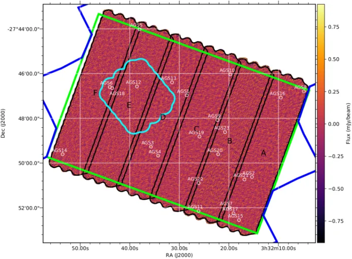
Our ALMA coverage extends over an effective area of 69 arcmin2 _{within the GOODS–South field (Fig. 1), centred at} α = 3h₃₂m_30.0s_{, δ= -27}◦ ₄₈0₀₀00_{(J2000; 2015.1.00543.S; PI:} D. Elbaz). To cover this ∼100_{× 7}0_{region (comoving scale of 15.1}

Mpc × 10.5 Mpc at z= 2), we designed a 846-pointing mosaic, each pointing being separated by 0.8 times the antenna Half Power Beam Width (i.e. HPBW ∼ 2300_{3). To accommodate such} large such a large number of pointings the ALMA Cycle 3 ob-serving mode restrictions, we divided this mosaic into six paral-lel, slightly overlapping, sub-mosaics of 141 pointing each. To get a homogeneous pattern over the 846 pointings, we computed the offsets between the sub-mosaics so that they connect with each other without breaking the hexagonal pattern of the ALMA mosaics.

Each sub-mosaic (or slice) has a length of 6.8 arcmin, a width of 1.5 arcmin and an inclination (PA) of 70 deg (see Fig.1). This required three execution blocks (EBs), yielding a total on-source integration time of ∼ 60 seconds per pointing (Table1). We determined that the highest frequencies of the band 6 is the optimal setup for a continuum survey and we thus set the ALMA correlator to Time Division Multiplexing (TDM) mode and optimised the setup for continuum detection at 264.9 GHz (λ= 1.13 mm) using four 1875 MHz-wide spectral windows cen-tered at 255.9 GHz, 257.9 GHz, 271.9 GHz and 273.9 GHz, cov-ering a total bandwidth of 7.5 GHz. The TDM mode has 128 channels per spectral window, providing us with ∼37 km/s ve-locity channels.

Observations were taken between the 1st_{of August and the} 2nd_{of September 2016, using ∼40 antennae (see Table1) in} con-figuration C40-5 with a maximum baseline of ∼ 1500 m. J0334-4008 and J0348-2749 (VLBA calibrator and hence has a highly precise position) were systematically used as flux and phase cal-ibrators, respectively. In 14 EBs, J0522-3627 was used as band-pass calibrator, while in the remaining 4 EBs J0238+1636 was used. Observations were taken under nominal weather condi-tions with a typical precipitable water vapour of ∼ 1 mm.

2.2. Data reduction

All EBs were calibrated with CASA (McMullin et al. 2007) us-ing the scripts provided by the ALMA project. Calibrated vis-ibilities were systematically inspected and few additional flag-gings were added to the original calibration scripts. Flux cali-brations were validated by verifying the accuracy of our phase and bandpass calibrator flux density estimations. Finally, to re-duce computational time for the forthcoming continuum imag-ing, we time- and frequency-averaged our calibrated EBs over 120 seconds and 8 channels, respectively.

Imaging was done in CASA using the multi-frequency synthesis algorithm implemented within the task CLEAN. Sub-mosaics were produced separately and combined subsequently using a weighted mean based on their noise maps. As each sub-mosaic was observed at different epochs and under differ-ent weather conditions, they exhibit different synthesized beams and sensitivities (Table1). Sub-mosaics were produced and pri-mary beam corrected separately, to finally be combined using a weighted mean based on their noise maps. To obtain a relatively homogeneous and circular synthesized beam across our final mosaic, we applied different u, v tapers to each sub-mosaic. The best balance between spatial resolution and sensitivity was found with a homogeneous and circular synthesized beam of 000₂₉ Full Width Half Maximum (FWHM; hereafter 00029-mosaic; Ta-ble1). We also applied this tapering method to create a second mosaic with an homogeneous and circular synthesized beam of 00060 FWHM (hereafter 00060-mosaic; Table1), i.e., optimised for the detection of extended sources. Mosaics with even coarser spatial resolution could not be created because of drastic sen-sitivity and synthesized beam shape degradations. In our 000

29-and 00060-mosaics, sidelobes of the synthesized beams do not carry much power as our brightest sources are at most detected at the 11-σ level (see Sect.4). We therefore perform our analysis on the dirty maps.

2.3. Building of the noise map

We build the RMS-map of the ALMA survey by a k-σ clipping method. In steps of 4 pixels on the image map, the standard de-viation was computed in a square of 100 × 100 pixels around the central pixel. The pixels, inside this box, with values greater than 3 times the standard deviation (σ) from the median value were masked. This procedure was repeated 3 times. Finally, we assign the value of the standard deviation of the non-masked pixels to the central pixel. This box size corresponds to the smallest size for which the value of the median pixel of the rms map con-verges to the typical value of the noise in the ALMA map while taking into account the local variation of noise. The step of 4 pixels corresponds to a sub-sampling of the beam so, the noise should not vary significantly on this scale. The median value of the standard deviation is 0.176 mJy.beam−1. In comparison, the Gaussian fit of the unclipped map gives a standard deviation of 0.182 mJy.beam−1. We adopt a general value of rms sensitivity σ = 0.18 mJy.beam−1_{. The average values for the 0}00_29-mosaic and the untapered mosaic are given in Table1.

2.4. Ancillary data

The area covered by this survey is ideally located, in that it prof-its from ancillary data from some of the deepest sky surveys at infrared (IR), optical and X-ray wavelengths. In this section, we describe all of the data that were used in the analysis of the ALMA detected sources in this paper.

2.4.1. Optical/near-infrared imaging

We have supporting data from the Cosmic Assembly Near-IR Deep Extragalactic Legacy Survey (CANDELS; Grogin et al. 2011) with images obtained with the Wide Field Camera 3/ in-frared channel (WFC3/IR) and UVIS channel, along with the Advanced Camera for Surveys (ACS; Koekemoer et al. 2011. The area covered by this survey lies in the deep region of the CANDELS program (central one-third of the field). The 5-σ de-tection depth for a point-source reaches a magnitude of 28.16 for the H160 filter (measured within a fixed aperture of 0.1700

Guo et al. 2013). The CANDELS/Deep program also provides

images in 7 other bands: the Y125, J125, B435, V606, i775, i814and z850filters, reaching 5-σ detection depths of 28.45, 28.35, 28.95, 29.35, 28.55, 28.84, and 28.77 mag respectively.

TheGuo et al.(2013) catalogue also includes galaxy mag-nitudes from the VLT, taken in the U-band with VIMOS (Nonino et al. 2009), and in the Ks-band with ISAAC (Retzlaff

et al. 2010) and HAWK-I (Fontana et al. 2014).

In addition, we use data coming from the FourStar Galaxy Evolution Survey (ZFOURGE, PI: I. Labbé) on the 6.5 m Magellan Baade Telescope. The FourStar instrument (Persson et al. 2013) observed the CDFS (encompassing the GOODS– South Field) through 5 near-IR medium-bandwidth filters (J1, J2, J3, Hs, Hl) as well as broad-band Ks. By combination of the FourStar observations in the Ks-band and previous deep and ultra-deep surveys in the K-band, VLT/ISAAC/K (v2.0) from GOODS (Retzlaff et al. 2010), VLT/HAWK-I/K from HUGS (Fontana et al. 2014), CFHST/WIRCAM/K from TENIS (Hsieh

et al. 2012) and Magellan/PANIC/K in HUDF (PI: I. Labbé), a

super-deep detection image has been produced. The ZFOURGE catalogue reaches a completeness greater than 80% to Ks< 25.3 - 25.9 (Straatman et al. 2016).

We use the stellar masses and redshifts from the ZFOURGE catalogue, except when spectroscopic redshifts are available. Stellar masses have been derived fromBruzual & Charlot(2003) models (Straatman et al. 2016) assuming exponentially declining star formation histories and a dust attenuation law as described byCalzetti et al.(2000).

2.4.2. Mid/far-infrared imaging

Data in the mid and far-IR are provided by the Infrared Ar-ray Camera (IRAC; Fazio et al. 2004) at 3.6, 4.5, 5.8, and 8 µm, Spitzer Multiband Imaging Photometer (MIPS; Rieke et al. 2004) at 24 µm, Herschel Photodetector Array Camera and Spectrometer (PACS,Poglitsch et al. 2010) at 70, 100 and 160 µm, and Herschel Spectral and Photometric Imaging RE-ceiver (SPIRE,Griffin et al. 2010) at 250, 350, and 500 µm.

The IRAC observations in the GOODS–South field were taken in February 2004 and August 2004 by the GOODS Spitzer Legacy project (PI: M. Dickinson). These data have been sup-plemented by the Spitzer Extended Deep Survey (SEDS; PI: G. Fazio) at 3.6 and 4.5 µm (Ashby et al. 2013) as well as the Spitzer-Cosmic Assembly Near-Infrared Deep Extragalactic Survey (S-CANDELS; Ashby et al. 2015) and recently by the ultradeep IRAC imaging at 3.6 and 4.5 µm (Labbé et al. 2015).

The flux extraction and deblending in 24 µm imaging have been provided by Magnelli et al. (2009) to reach a depth of S24 ∼30 µJy. Herschel images come from a 206.3 h GOODS– Southobservational program (Elbaz et al. 2011) and combined by Magnelli et al. (2013) with the PACS Evolutionary Probe (PEP) observations (Lutz et al. 2011). Because the SPIRE confu-sion limit is very high, we use the catalogue of T. Wang et al. (in prep), which is built with a state-of-the art de-blending method using optimal prior sources positions from 24 µm and Herschel PACS detections.

2.4.3. Complementary ALMA data

As the GOODS–South Field encompasses the Hubble Ultra Deep Field (HUDF), we take advantage of deep 1.3-mm ALMA data of the HUDF. The ALMA image of the full HUDF reaches a σ1.3mm= 35 µJy (Dunlop et al. 2017), over an area of 4.5 arcmin2 that was observed using a 45-pointing mosaic at a tapered res-olution of 0.700. These observations were taken in two separate periods from July to September 2014. In this region, 16 galax-ies were detected byDunlop et al.(2017), 3 of them with a high SNR (SNR > 14), the other 13 with lower SNRs (3.51 < SNR < 6.63).

2.4.4. Radio imaging

We also use radio imaging at 5 cm from the Karl G. Jansky Very Large Array (JVLA). These data were observed during 2014 March - 2015 September for a total of 177 hours in the A, B, and C configurations (PI: W. Rujopakarn). The images have a 00031 × 00061 synthesized beam and an rms noise at the point-ing centre of 0.32 µJy.beam−1_{(Rujopakarn et al. 2016). Here, 179} galaxies were detected with a significance greater than 3 σ over an area of 61 arcmin2_{around the HUDF field, with a rms}

sensi-Original Mosaic 000

29-Mosaic 000

60-Mosaic

Slice Date # t on target total t Beam σ Beam σ Beam σ

min min mas × mas µJy.beam−1 _{mas × mas µJy.beam}−1 _{mas × mas µJy.beam}−1

A August 17 42 46.52 72.12 240 × 200 98 297 × 281 108 618 × 583 171 August 31 39 50.36 86.76 August 31 39 46.61 72.54 B September 1 38 46.87 72.08 206 × 184 113 296 × 285 134 614 × 591 224 September 1 38 48.16 72.48 September 2 39 46.66 75.06 C August 16 37 46.54 73.94 243 × 231 102 295 × 288 107 608 × 593 166 August 16 37 46.54 71.58 August 27 42 46.52 74.19 D August 16 37 46.54 71.69 257 × 231 107 292 × 289 111 612 × 582 164 August 27 44 46.52 72.00 August 27 44 46.52 72.08 E August 01 39 46.54 71.84 285 × 259 123 292 × 286 124 619 × 588 186 August 01 39 46.53 72.20 August 02 40 46.53 74.46 F August 02 40 46.53 72.04 293 × 256 118 292 × 284 120 613 × 582 178 August 02 41 46.53 71.61 August 02 39 46.53 71.55 Mean 40 46.86 73.35 254 × 227 110 294 × 286 117 614 × 587 182

Table 1. Summary of the observations. The slice ID, the date, the number of antennae, the time on target, the total time (time on target+ calibration time), the resolution and the 1-σ noise of the slice are given.

Fig. 1. ALMA 1.1 mm image tapered at 000

60. The white circles have a diameter of 4 arcseconds and indicate the positions of the galaxies listed in Table3. Black contours show the different slices (labelled A to F) used to compose the homogeneous 1.1 mm coverage, with a median

RMS-noise of 0.18 mJy per beam. Blue lines show the limits of the HST/ACS field and green lines indicate the HST-WFC3 deep region. The cyan contour represents the limit of theDunlop et al.(2017) survey covering all the Hubble Ultra Deep Field region. All of the ALMA-survey field is encompassed by the Chandra Deep Field-South.

tivity better than 1 µJy.beam−1. However, this radio survey does not cover the entire ALMA area presented in this paper. 2.4.5. X-ray

The Chandra Deep Field-South (CDF-S) was observed for 7 Msec between 2014 June and 2016 March. These observa-tions cover a total area of 484.2 arcmin2_{, offset by just 32}00_from the centre of our survey, in three X-ray bands: 0.5-7.0 keV, 0.5-2.0 keV, and 2-7 keV (Luo et al. 2017). The average flux limits over the central region are 1.9 × 10−17_{, 6.4 × 10}−18_{, and} 2.7 × 10−17erg cm−2 s−1respectively. This survey enhances the previous X-ray catalogues in this field, the 4 Msec Chandra ex-posure (Xue et al. 2011) and the 3 Msec XMM-Newton exposure (Ranalli et al. 2013). We will use this X-ray catalogue to identify candidate X-ray active galactic nuclei (AGN) among our ALMA detections.

3. Source Detection

The search for faint sources in high-resolution images with mod-erate source densities faces a major limitation. At the native reso-lution (00025 × 00023), the untapered ALMA mosaic encompasses almost 4 million independent beams, where the beam area is Abeam= π × FWHM2/(4ln(2)). It results that a search for sources above a detection threshold of 4-σ would include as many as 130 spurious sources assuming a Gaussian statistics. Identifying the real sources from such catalogue is not possible. In order to increase the detection quality to a level that ensures a purity greater than 80% – i.e., the excess of sources in the original mo-saic needs to be 5 times greater than the number of detections in the mosaic multiplied by (-1) – we have decided to use a tapered image and adapt the detection threshold accordingly.

By reducing the weight of the signal originating from the most peripheral ALMA antennae, the tapering reduces the an-gular resolution hence the number of independent beams at the expense of collected light. The lower angular resolution presents the advantage of optimizing the sensitivity to point sources – we recall that 00024 corresponds to a proper size of only 2 kpc at z∼1–3 – and therefore will result in an enhancement of the signal-to-noise ratio for the sources larger than the resolution.

We chose to taper the image with an homogeneous and cir-cular synthesized beam of 00060 FWHM – corresponding to a proper size of 5 kpc at z∼1–3 – after having tested various ker-nels and found that this beam was optimised for our mosaic, avoiding both a beam degradation and a too heavy loss of sen-sitivity. This tapering reduces by nearly an order of magnitude the number of spurious sources expected at a 4-σ level down to about 19 out of 600 000 independent beams. However, we will check in a second step whether we may have missed in the process some compact sources by analysing as well the 000₂₉ tapered map.

We also excluded the edges of the mosaic, where the standard deviation is larger than 0.30 mJy.beam−1 _{in the 0}00_60-mosaic. The effective area is thus reduced by 4.9% as compared to the full mosaic (69.46 arcmin2_{out of 72.83 arcmin}2_).

To identify the galaxies present on the image, we use Blob-cat (Hales et al. 2012). Blobcat is a source extraction software using a "flood fill" algorithm to detect and catalogue blobs (see

Hales et al. 2012). A blob is defined by two criteria: – at least one pixel has to be above a threshold (σp)

– all the adjacent surrounding pixels must be above a floodclip threshold (σf)

5.0

2.5 0.0

2.5

5.0

7.5 10.0

SNR

10

10

10

10

10

10

10

N

-0.90 -0.45 0.00 0.45 0.90 1.35 1.80

S

[mJy.beam

]

Fig. 2. Histogram of pixels of the signal to noise map, where pixels with noise > 0.3 mJy.beam−1_{have been removed. The red dashed line is the}

best Gaussian fit. The green dashed line is indicative and shows where the pixel brightness distribution moves away from the Gaussian fit. This is also the 4.2 σ level corresponding to a peak flux of 0.76 mJy for a typical noise per beam of 0.18 mJy. The solid black line corresponds to our peak threshold of 4.8 σ (0.86 mJy).

where σpand σf are defined in number of σ, the local RMS of the mosaic.

A first guess to determine the detection threshold σpis pro-vided by the examination of the pixel distribution of the signal to noise map (SNR-map). The SNR-map has been created by divid-ing the 000_{60 tapered map by the noise map. Fig.2shows that the} SNR-map follows an almost perfect Gaussian below SNR= 4.2. Above this threshold, a significant difference can be observed that is characteristic of the excess of positive signal expected in the presence of real sources in the image. However, this his-togram alone cannot be used to estimate a number of sources because the pixels inside one beam are not independent from one another. Hence although the non Gaussian behaviour ap-pears around SNR= 4.2 we perform simulations to determine the optimal values of σpand σf.

We first conduct positive and negative – on the continuum map multiplied by (-1) – detection analysis for a range of σp and σf values ranging from σp= 4 to 6 and σf= 2.5 to 4 with intervals of 0.05 and imposing each time σp≥σf. The difference between positive and negative detections for each pair of (σp, σf) values provides the expected number of real sources.

Then we search for the pair of threshold parameters to find the best compromise between (i) providing the maximum number of detections, and (ii) minimising the number spurious sources. The later purity criterion, pc, is defined as:

pc =

Np− Nn Np

(1) where Npand Nnare the numbers of positive and negative detec-tions respectively. To ensure a purity of 80% as discussed above, we enforce pc ≥ 0.8. This leads to σp= 4.8 σ when fixing the value of σf= 2.7 σ (see Fig.3-left). Below σp= 4.8 σ, the purity criterion rapidly drops below 80% whereas above this value it only mildly rises. Fixing σp= 4.8 σ, the purity remains roughly constant at ∼80±5% when varying σf. We do see an increase in the difference between the number of positive and negative detections with increasing σf. However, the size of the sources

above σf= 2.7 σ drops below the 00060 FWHM and tends to be-come pixel-like, hence non physical. This is due to the fact that an increase of σf results in a reduction of the number of pixels above the floodclip threshold (σf) that will be associated to a given source. This parameter can be seen as a percolation cri-terion that sets the size of the sources in number of pixels. Re-versely reducing σf below 2.7 σ results in adding more noise than signal and in reducing the number of detections. We there-fore decided to set σf to 2.7 σ.

While we do not wish to impose a criterion on the exis-tence of optical counterparts to define our ALMA catalogue, we do find that high values of σf not only generates the problem discussed above, but also generates a rapid drop of the frac-tion of ALMA detecfrac-tions with an HST counterpart in theGuo et al.(2013) catalogue, pHS T= NHS T/Np. NHS T is the number of ALMA sources with an HST counterpart within 00060 (cor-responding to the size of the beam). The fraction falls rapidly from around ∼80% to ∼60%, which we interpret as being due to a rise of the proportion of spurious sources since the faintest op-tical sources, e.g., detected by HST-WFC3, are not necessarily associated with the faintest ALMA sources due to the negative k-correction at 1.1mm. This rapid drop can be seen in the dashed green and dotted pink lines of Fig.3-right. This confirms that the sources that are added to our catalogue with a floodclip thresh-old greater than 2.7 σ are most probably spurious. Similarly, we can see in Fig.3-left that increasing the number of ALMA detec-tions to fainter flux densities by reducing σp below 4.8 σ leads to a rapid drop of the fraction of ALMA detections with an HST counterpart. Again there is no well-established physical reason to expect the number of ALMA detections with an optical coun-terpart to decrease with decreasing S/N ratio in the ALMA cata-logue.

Hence we decided to set σp= 4.8 σ and σf= 2.7 σ to pro-duce our catalogue of ALMA detections. We note that we only discussed the existence of HST counterparts as a complementary test on the definition of the detection thresholds but our approach is not set to limit in any way our ALMA detections to galaxies with HST counterparts.

Indeed, evidence for the existence of ALMA detections with no HST-WFC3 counterparts already exist in the literature.Wang et al. (2016) identified H-dropouts galaxies, i.e. galaxies de-tected above the H-band with Spitzer-IRAC at 4.5 µm but unde-tected in the H-band and in the optical. The median flux density of these galaxies is F870µm ' 1.6 mJy (T. Wang et al., in prep.). By scaling this median value to our wavelength of 1.1 mm (the details of this computation are given in Sect.5.4), we obtain a flux density of 0.9 mJy, close to the typical flux of our detections (median flux ∼1 mJy, see Table3).

4. Catalogue

4.1. Creation of the catalogue

Using the optimal parameters of σp= 4.8 σ and σf= 2.7 σ de-scribed in Sect.3, we obtain a total of 20 detections down to a flux density limit of S1.1mm ≈ 880 µJy that constitute our main catalogue. These detections can be seen ranked by their SNR in Fig.1. The comparison of negative and positive detections sug-gests the presence of 4±2 (assuming a Poissonian uncertainty on the difference between the number of positive and negative detections) spurious sources in this sample.

In the following, we assume that the galaxies detected in the 00060-mosaic are point-like. This hypothesis will later on be discussed and justified in Sect. 4.5. In order to check

the robustness of our flux density measurements, we com-pared different flux extraction methods and softwares: PyBDSM (Mohan & Rafferty 2015); Galfit (Peng et al. 2010); Blobcat (Hales et al. 2012). The peak flux value determined by Blobcat refers to the peak of the surface brightness corrected for peak bias (see Hales et al. 2012). The different results are con-sistent, with a median ratio of FBlobcat

peak /F PyBDSM peak = 1.04±0.20 and FBlobcat peak /F Galfit

PS F = 0.93±0.20. The flux measured using psf-fitting (Galfit) and peak flux measurement (Blobcat) for each galaxy are listed in Table3. We also ran CASA fitsky and a sim-ple aperture photometry corrected for the ALMA PSF and also found consistent results. The psf-fitting with Galfit was per-formed inside a box of 5×500_{centred on the source.}

The main characteristics of these detections (redshift, flux, SNR, stellar mass, counterpart) are given in Table 3. We use redshifts and stellar masses from the ZFOURGE catalogue (see Sect.2.4.1).

We compare the presence of galaxies between the 000 60-mosaic and the 000_{29-mosaic. Of the 20 detections found in the} 00060 map, 14 of them are also detected in the 00029 map. The presence of a detection in both maps reinforces the plausibility of a detection. However, a detection in only one of these two maps may be a consequence of the intrinsic source size. An ex-tended source is more likely to be detected with a larger beam, whereas a more compact source is more likely to be missed in the maps with larger tapered sizes and reduced point source sen-sitivity.

A first method to identify potential false detections is to com-pare our results with a deeper survey overlapping with our area of the sky. We compare the positions of our catalogue sources with the positions of sources found byDunlop et al.(2017) in the HUDF. This 1.3-mm image is deeper than our survey and reaches a σ ' 35 µJy (corresponding to σ= 52 µJy at 1.1mm) but overlaps with only ∼6.5% of our survey area. The final sample ofDunlop et al.(2017) was compiled by selecting sources with S1.3 > 120 µJy to avoid including spurious sources due to the large number of beams in the mosaics and due to their choice of including only ALMA detections with optical counterpart seen with HST.

With our flux density limit of S1.1mm ≈ 880 µJy any non-spurious detection should be associated to a source seen at 1.3mm in the HUDF 1.3 mm survey, the impact of the wave-length difference being much smaller than this ratio. We de-tect 3 galaxies that were also dede-tected byDunlop et al.(2017), UDF1, UDF2 and UDF3, all of which having S1.3mm> 0.8 mJy. The other galaxies detected byDunlop et al.(2017) have a flux density at 1.3 mm lower than 320 µJy, which makes them unde-tectable with our sensitivity.

We note however that we did not impose as a strict criterion the existence of an optical counterpart to our detections whereas

Dunlop et al.(2017) did. Hence if we had detected a source with no optical counterpart within the HUDF, this source may not be included in theDunlop et al.(2017) catalogue. However, as we will see, the projected density of such sources is small and none of our candidate optically dark sources falls within the limited area of the HUDF. We also note that the presence of an HST-WFC3 source within a radius of 0006 does not necessarily imply that is the correct counterpart. As we will discuss in detail in Sect. 4.4, due to the depth of the HST-WFC3 observation and the large number of galaxies listed in the CANDELS catalogue, a match between the HST and ALMA positions may be possible by chance alignment alone (see Sect.4.4).

4.00 4.25 4.50 4.75 5.00 5.25 5.50 5.75 6.00

(

= 2.7)

10

10

10

N

0.0

0.2

0.4

0.6

0.8

1.0

p

,

p

,

p

2.50

2.75

3.00

3.25

3.50

3.75

4.00

(

= 4.8)

0

10

20

30

40

N

0.0

0.2

0.4

0.6

0.8

1.0

p

,

p

,

p

Fig. 3. Cumulative number of positive (red histogram) and negative (blue histogram) detections as a function of the σp(at a fixed σf, left panel)

and σf (at a fixed σp, right panel) in units of σ. Solid black line represents the purity criterion pcdefine by Eq.1, green dashed-line represents the

percentage of positive detection with HST-WFC3 counterpart pHS Tand magenta dashed-line represents the percentage of positive detection with

ZFOURGE counterpart pZFOURGE. Grey dashed-lines show the thresholds σp= 4.8 σ and σf= 2.7 σ and the 80% purity limit.

ID IDCLS IDZF RAALMA DecALMA RAHS T DecHS T ∆HS T1 ∆HS T2 (∆α)HS T (∆δ)HS T ∆IRAC

deg deg deg deg arcsec arcsec arcsec arcsec arcsec

(1) (2) (3) (4) (5) (6) (7) (8) (9) (10) (11) (12) AGS1 14876 17856 53.118815 -27.782889 53.118790 -27.782818 0.27 0.03 0.091 -0.278 0.16 AGS2 7139 10316 53.063867 -27.843792 53.063831 -27.843655 0.51 0.23 0.163 -0.269 0.04 AGS3 9834 13086 53.148839 -27.821192 53.148827 -27.821121 0.26 0.06 0.099 -0.262 0.10 AGS4 8923b 12333 53.142778 -27.827888 53.142844 -27.827890 0.21 0.40 0.087 -0.264 0.09 AGS5 20765 23898 53.158392 -27.733607 53.158345 -27.733485 0.46 0.13 0.087 -0.329 0.26 AGS6 15669 - 53.183458 -27.776654 53.183449 -27.776584 0.26 0.03 0.054 -0.267 0.40 AGS7 4854 7867 53.082738 -27.866577 53.082705 -27.866567 0.11 0.19 0.124 -0.225 0.03 AGS8 15261 18282 53.020356 -27.779905 53.020297 -27.779829 0.33 0.03 0.159 -0.275 0.20 AGS9 12016 15639 53.092844 -27.801330 53.092807 -27.801208 0.45 0.16 0.100 -0.276 0.18 AGS10 16972 19833 53.082118 -27.767299 53.081957 -27.767202 0.62 0.39 0.128 -0.300 0.40 AGS11 - 7589 53.108818 -27.869055 - - - 0.12 AGS12 15876 18701 53.160634 -27.776273 53.160594 -27.776129 0.53 0.28 0.076 -0.242 0.51 AGS13 16274 19033 53.131122 -27.773194 53.131080 -27.773108 0.34 0.05 0.087 -0.291 0.14 AGS14 - - 53.223156 -27.826771 - - - -AGS15 3818b 6755 53.074847 -27.875880 53.074755 -27.875976 0.45 0.57 0.125 -0.195 0.121 AGS16 - - 53.039724 -27.784557 - - - -AGS17 4414b 6964 53.079374 -27.870770 53.079327 -27.870781 0.16 0.27 0.122 -0.231 0.06 AGS18 15639 18645 53.181355 -27.777544 53.181364 -27.777501 0.16 0.12 0.043 -0.256 0.10 AGS19 - - 53.108041 -27.813610 - - - -AGS20 9089 12416 53.092365 -27.826829 53.092381 -27.826828 0.05 0.29 0.116 -0.247 0.18 AGS21 6905 10152 53.070274 -27.845586 53.070230 -27.845533 0.24 0.06 0.143 -0.249 0.07 AGS22 28952 - 53.108695 -27.848332 53.108576 -27.848242 0.50 0.29 0.106 -0.226 -AGS23 10954 14543 53.086623 -27.810272 53.086532 -27.810217 0.35 0.19 0.111 -0.263 0.16 Table 2. Details of the positional differences between ALMA and HST-WFC3 for our catalogue of galaxies identified in the 1.1mm-continuum map. Columns: (1) Source ID; (2),(3) IDs of the HST-WFC3 (from the CANDELS catalogue) and ZFOURGE counterparts of these detections (the cross correlations between ALMA and HST-WFC3 and between ALMA and ZFOURGE are discussed in Sect. 4.4). b indicates HST-WFC3 galaxies located in a radius of 000

6 around the ALMA detection, although strong evidence presented in Sect.7suggests they are not the optical counterparts of our detections; (4), (5) RA and Dec of the sources in the ALMA image (J2000); (6), (7) Positions of HST-WFC3 H-band counterparts when applicable fromGuo et al.(2013), (8), (9) Distances between the ALMA and HST source positions before (∆HS T1) and

after(∆HS T2) applying the offset correction derived from the comparison with Pan-STARRS and GAIA; (10), (11) Offset to be applied to the HST

source positions, which includes both the global systematic offset and the local offset; (12) Distance from the closest IRAC galaxy.1_{For AGS15}

we use the distance given in the ZFOURGE catalogue (see Sect.7).

4.2. Supplementary catalogue

After the completion of the main catalogue, three sources that did not satisfy the criteria of the main catalogue presented strong evidences of being robust detections. We therefore enlarged our catalogue, in order to incorporate these sources into a supple-mentary catalogue.

These three sources are each detected using a combination of σpand σfgiving a purity factor greater than 80%, whilst also ensuring the existence of an HST counterpart.

The galaxy AGS21 has an SNR= 5.83 in the 000_{29 tapered} map, but is not detected in the 00060 tapered map. The non-detection of this source is most likely caused by its size. Due to its dilution in the 00060-mosaic, a very compact galaxy detected at 5 σ in the 000_{29-mosaic map could be below the detection limit}

in the 00060-mosaic. The ratio of the mean RMS of the two ta-pered maps is 1.56, meaning that for a point source of certain flux, a 5.83 σ measurement in the 000_{29-mosaic becomes 3.74 σ} in the 00060-map.

The galaxy AGS22 has been detected with an SNR= 4.9 in the 00060 tapered map (σp= 4.9 and σf= 3.1). With σpand σf values more stringent than the thresholds chosen for the main catalogue, it may seem paradoxical that this source does not ap-pear in the main catalogue. With a floodclip criterion of 2.7 σ, this source would have an SNR just below 4.8 excluding it from the main catalogue. This source is associated with a faint galaxy that has been detected by HST-WFC3 (IDCANDELS = 28952) at 1.6 µm (6.6 σ) at a position close to the ALMA detection (00028). Significant flux has also been measured at 1.25 µm (3.6 σ) for this galaxy. In all of the other filters, the flux measurement is not significant (< 3 σ). Due to this lack of information, it has not been possible to compute its redshift. AGS22 is not detected in the 000_{29-mosaic map with p}

c> 0.8. This is the only galaxy (except the three galaxies most likely to be spurious: AGS14, AGS16 and AGS19) that has not been detected by IRAC.

The galaxy AGS23 was detected in the 00060 map just below our threshold at 4.8 σ, with a combination σp= 4.6 and σf= 2.9 giving a purity criterion greater than 0.9. This detection is associ-ated with an HST-WFC3 counterpart. It is for these two reasons that we include this galaxy in the supplementary catalogue. The photometric redshift (z= 2.36) and stellar mass (1011.26M) both reinforce the plausibility of this detection.

4.3. Astrometric correction

The comparison of our ALMA detections with HST (Sect.4.1) in the previous section was carried out after correcting for an astro-metric offset, which we outline here. In order to perform the most rigorous counterpart identification and take advantage of the ac-curacy of ALMA, we carefully investigated the astrometry of our images. Before correction, the galaxy positions viewed by HST are systematically offset from the ALMA positions. This offset has already been identified in previous studies (e.g. Maiolino et al. 2015;Rujopakarn et al. 2016;Dunlop et al. 2017).

In order to quantify this effect, we compared the HST source positions with detections from the Panoramic Survey Telescope and Rapid Response System (Pan-STARRS). This survey has the double advantage to cover a large portion of the sky, notably the GOODS–South field, and to observe the sky at a wavelength similar to HST-WFC3. We use the Pan-STARRS DR1 catalogue provided byFlewelling et al.(2016) and also include the corre-sponding regions issued from the GAIA DR1 (Gaia Collabora-tion et al. 2016).

Cross-matching was done within a radius of 0005. In order to minimize the number of false identifications, we subtracted the median offset between the two catalogues from theGuo et al.

(2013) catalogue positions, after the first round of matching. We iterated this process three times. In this way, 3 587 pairs were found over the GOODS–South field.

To correct for the median offset between the HST and ALMA images, the HST image coordinates must be corrected by −94±42 mas in right ascension, α, and 262±50 mas in declina-tion, δ, where the uncertainties correspond to the standard devi-ation of the 3 587 offset measurements. This offset is consistent with that found byRujopakarn et al.(2016) of∆α = −80±110 mas and∆δ = 260±130 mas. The latter offsets were calculated by comparing the HST source positions with 2MASS and VLA positions. In all cases, it is the HST image that presents an offset, whereas ALMA, Pan-STARRS, GAIA, 2MASS and VLA are all

0.6

0.4

0.2

0.0

0.2

0.4

0.6

["]

0.6

0.4

0.2

0.0

0.2

0.4

0.6

["

]

Before correction

After correction

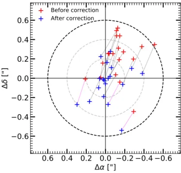
Fig. 4. Positional offset (RAHS T - RAALMA, DECHS T - DECALMA)

be-tween HST and ALMA before (red crosses) and after (blue crosses) the correction of both a global systematic offset and a local offset. The black dashed circle corresponds to the cross-matching limit radius of 000

6. The grey dashed circles show a positional offset of 000

2 and 000

4 respectively. The magenta lines indicate the HST galaxies previously falsely associated with ALMA detections.

in agreement. We therefore deduce that it is the astrometric solu-tion used to build the HST mosaic that introduced this offset. As discussed in Dickinson et al. (in prep.), the process of building the HST mosaic also introduced less significant local offsets, that can be considered equivalent to a distortion of the HST image. These local offsets are larger in the periphery of GOODS–South than in the centre, and close to zero in the HUDF field. The local offsets can be considered as a distortion effect. The offsets listed in Table2include both effects, i.e., the global and local offsets. The separation between HST and ALMA detections before and after offset correction, and the individual offsets applied for each of the galaxies are indicated in Table 2 and can be visualized in Fig.4. We applied the same offset corrections to the galaxies listed in the ZFOURGE catalogue.

This accurate subtraction of the global systematic offset as well as the local offset does not however guarantee a perfect overlap between ALMA and HST emission. The location of the dust emission may not align perfectly with the starlight from a galaxy, due to the difference in ALMA and HST resolutions, as well as the physical offsets between dust and stellar emission that may exist. In Fig. 5, we show the ALMA contours (4 to 10 σ) overlaid on the F160W HST-WFC3 images after astro-metric correction. In some cases (AGS1, AGS3, AGS6, AGS13, AGS21 for example), the position of the dust radiation matches that of the stellar emission; in other cases, (AGS4, AGS17 for ex-ample), a displacement appears between both two wavelengths. Finally, in some cases (AGS11, AGS14, AGS16, and AGS19) there are no optical counterparts. We will discuss the possible explanations for this in Sect.7.

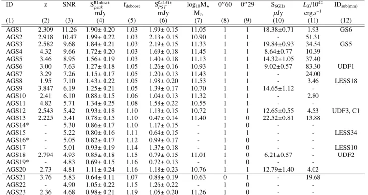
ID z SNR SBlobcat

peak fdeboost S Galfit

PS F log10M? 00060 00029 S6GHz LX/1042 IDsub(mm)

mJy mJy M µJy erg.s−1

(1) (2) (3) (4) (5) (6) (7) (8) (9) (10) (11) (12) AGS1 2.309 11.26 1.90± 0.20 1.03 1.99± 0.15 11.05 1 1 18.38±0.71 1.93 GS6 AGS2 2.918 10.47 1.99± 0.22 1.03 2.13± 0.15 10.90 1 1 - 51.31 AGS3 2.582 9.68 1.84± 0.21 1.03 2.19± 0.15 11.33 1 1 19.84±0.93 34.54 GS5 AGS4 4.32 9.66 1.72± 0.20 1.03 1.69± 0.18 11.45 1 1 8.64±0.77 10.39 AGS5 3.46 8.95 1.56± 0.19 1.03 1.40± 0.18 11.13 1 1 14.32±1.05 37.40 AGS6 3.00 7.63 1.27± 0.18 1.05 1.26± 0.16 10.93 1 1 9.02±0.57 83.30 UDF1 AGS7 3.29 7.26 1.15± 0.17 1.05 1.20± 0.13 11.43 1 1 - 24.00 AGS8 1.95 7.10 1.43± 0.22 1.05 1.98± 0.20 11.53 1 1 - 3.46 LESS18 AGS9 3.847 6.19 1.25± 0.21 1.05 1.39± 0.17 10.70 1 1 14.65±1.12 -AGS10 2.41 6.10 0.88± 0.15 1.06 1.04± 0.13 11.32 1 1 - 2.80 AGS11 4.82 5.71 1.34± 0.25 1.08 1.58± 0.22 10.55 1 1 - -AGS12 2.543 5.42 0.93± 0.18 1.10 1.13± 0.15 10.72 1 1 12.65±0.55 4.53 UDF3, C1 AGS13 2.225 5.41 0.78± 0.15 1.10 0.47± 0.14 11.40 1 0 22.52±0.81 13.88 AGS14* - 5.30 0.86± 0.17 1.10 1.17± 0.15 - 1 0 - -AGS15 - 5.22 0.80± 0.16 1.11 0.64± 0.15 - 1 1 - - LESS34 AGS16* - 5.05 0.82± 0.17 1.12 0.99± 0.17 - 1 0 - -AGS17 - 5.01 0.93± 0.19 1.14 1.37± 0.18 - 1 0 - - LESS10 AGS18 2.794 4.93 0.85± 0.18 1.15 0.79± 0.15 11.01 1 0 6.21±0.57 - UDF2 AGS19* - 4.83 0.69± 0.15 1.16 0.72± 0.13 - 1 0 - -AGS20 2.73 4.81 1.11± 0.24 1.16 1.18± 0.23 10.76 1 1 12.79±1.40 4.02 AGS21 3.76 5.83 0.64± 0.11 1.07 0.88± 0.19 10.63 0 1 - 19.68 AGS22 - 4.90 1.05± 0.22 1.15 1.26± 0.22 - 1 0 - -AGS23 2.36 4.68 0.98± 0.21 1.19 1.05± 0.20 11.26 1 0 -

-Table 3. Details of the final sample of sources detected in the ALMA GOODS–South continuum map, from the primary catalogue in the main part of the table and from the supplementary catalogue below the solid line (see Sect.4.1and Sect.4.2). Columns: (1) IDs of the sources as shown in Fig.1. The sources are sorted by SNR. * indicates galaxies that are most likely spurious, i.e., not detected at any other wavelength; (2) Redshifts from the ZFOURGE catalogue. Spectroscopic redshifts are shown with three decimal places. As AGS6 is not listed in the ZFOURGE catalogue, we use the redshift computed byDunlop et al.(2017); (3) Signal to noise ratio of the detections in the 000

60 mosaic (except for AGS21). This SNR is computed using the flux from Blobcat and is corrected for peak bias; (4) Peak fluxes measured using Blobcat in the 000

60-mosaic image before de-boosting correction; (5) Deboosting factor; (6) Fluxes measured by PSF-fitting with Galfit in the 000

60-mosaic image before de-boosting correction; (7) Stellar masses from the ZFOURGE catalogue; (8), (9) Flags for detection by Blobcat in the 000

60-mosaic and 000

29-mosaic images, where at least one combination of σpand σf gives a purity factor (Eq.1) greater than 80%; (10) Flux for detection greater than

3 σ by JVLA (5 cm). Some of these sources are visible in the JVLA image but not detected with a threshold > 3 σ. AGS8 and AGS16 are not in the field of the JVLA survey; (11) Absorption-corrected intrinsic 0.5-7.0 keV luminosities. The X-ray luminosities have been corrected to account for the redshift difference between the redshifts provided in the catalogue ofLuo et al.(2017) and those used in the present table, when necessary. For this correction we used Eq. 1 fromAlexander et al.(2003), and assuming a photon index ofΓ = 2; (12) Corresponding IDs for detections of the sources in previous (sub)millimetre ancillary data. UDF is for Hubble Ultra Deep Field survey (Dunlop et al. 2017) at 1.3 mm, C indicates the ALMA Spectroscopic Survey in the Hubble Ultra Deep Field (ASPECS) at 1.2 mm (Aravena et al. 2016), LESS indicates data at 870 µm presented inHodge et al.(2013) and GS indicates data at 870 µm presented inElbaz et al.(2017).

4.4. Identification of counterparts

We searched for optical counterparts in the CANDELS/GOODS–South catalogue, within a radius of 000_{6 from the millimetre position after having applied the} astro-metric corrections to the source positions described in Sect.4.3. The radius of the cross-matching has been chosen to correspond to the synthesized beam (000_{60) of the tapered ALMA map used} for galaxy detection. Following Condon (1997), the maximal positional accuracy of the detection in the 1.1mm map is given by θbeam/(2×SNR). In the 00060-mosaic, the positional accuracy therefore ranges between 26.5 mas and 62.5 mas for our range of SNR (4.8-11.3), corresponding to physical sizes between 200 and 480 pc at z= 3.

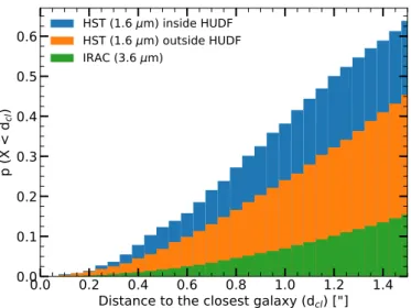
Despite the high angular resolution of ALMA, the chance of an ALMA-HST coincidence is not negligible, because of the large projected source density of the CANDELS/GOODS–South catalogue. Fig.6shows a Monte Carlo simulation performed to estimate this probability. We separate here the deeper Hubble Ul-tra Deep Field (blue histogram) from the rest of the CANDELS-Deep area (orange histogram). We randomly define a position within GOODS–South and then measure the distance to its clos-est HST neighbour using the source positions listed inGuo et al.

(2013). We repeat this procedure 100 000 times inside and out-side the HUDF. The probability for a position randomly selected in the GOODS–South field to fall within 0.6 arcsec of an HST source is 9.2% outside the HUDF, and 15.8% inside the HUDF. We repeat this exercise to test the presence of an IRAC counter-part with the Ashby et al.(2015) catalogue (green histogram). The probability to randomly fall on an IRAC source is only 2.1%.

With the detection threshold determined in Sect.3, 80% of the millimetre galaxies detected have an HST-WFC3 counter-part, and 4 galaxies remain without an optical counterpart. We cross-matched our detections with the ZFOURGE catalogue.

Fig. 7 shows 300_{5 × 3.}00_{5 postage stamps of the} ALMA-detected galaxies, overlaid with the positions of galaxies from the CANDELS/GOODS–South catalogue (magenta double crosses), ZFOURGE catalogue (white circles) or both catalogues (i.e. sources with an angular separation lower than 0004, blue cir-cles). These are all shown after astrometric correction. Based on the ZFOURGE catalogue, we find optical counterparts for one galaxy that did not have an HST counterpart: AGS11, a photo-metric redshift has been computed in the ZFOURGE catalogue for this galaxy.

53°07'07" 08" 59.0" 58.5" -27°46'58.0" Dec (J2000) AGS1 53°03'49" 50" 51" 38.5" 38.0" 37.5" -27°50'37.0" AGS2 53°08'55" 56" 17.0" 16.5" 16.0" -27°49'15.5" AGS3 53°08'34" 35" 41.0" 40.5" 40.0" -27°49'39.5" AGS4 53°09'30" 31" 01.5" 01.0" -27°44'00.5" Dec (J2000) AGS5 53°11'00" 01" 36.5" 36.0" -27°46'35.5" AGS6 53°04'57" 58" 00.5" 52'00.0" 59.5" -27°51'59.0" AGS7 53°01'13" 14" 48.5" 48.0" 47.5" -27°46'47.0" AGS8 53°05'34" 35" 05.5" 05.0" 04.5" -27°48'04.0" Dec (J2000) AGS9 53°04'55" 56" 03.0" 02.5" 02.0" -27°46'01.5" AGS10 53°06'31" 32" 09.5" 09.0" 08.5" -27°52'08.0" AGS11 53°09'38" 39" 35.5" 35.0" 34.5" -27°46'34.0" AGS12 53°07'52" 53" 24.0" 23.5" -27°46'23.0" Dec (J2000) AGS13 53°13'23" 24" 37.0" 36.5" 36.0" -27°49'35.5" _AGS14 53°04'29" 30" 34.0" 33.5" 33.0" -27°52'32.5" AGS15 53°02'22" 23" 24" 05.0" 04.5" -27°47'04.0" AGS16 53°04'45" 46" 15.5" 15.0" 14.5" -27°52'14.0" Dec (J2000) AGS17 53°10'52" 53" 40.0" 39.5" 39.0" -27°46'38.5" AGS18 53°06'28" 29" 30" 49.5" 49.0" -27°48'48.5" AGS19 53°05'32" 33" 37.5" 37.0" 36.5" -27°49'36.0" AGS20 53°04'12" 13" 14" RA (J2000) 45.0" 44.5" 44.0" -27°50'43.5" Dec (J2000) AGS21 53°06'31" 32" RA (J2000) 54.5" 54.0" -27°50'53.5" AGS22 53°05'11" 12" RA (J2000) 37.5" 37.0" -27°48'36.5" AGS23

Fig. 5. Postage stamps of 1.8 × 1.8 arcsec. ALMA contours (4, 4.5 then 5 to 10-σ with a step of 1-σ) at 1.1mm (white lines) are overlaid on F160W HST/WFC3 images. The images are centred on the ALMA detections. The shape of the synthesized beam is given in the bottom left corner. Astrometry corrections described in Sect.4.3have been applied to the HST images. In some cases (AGS1, AGS3, AGS6, AGS13, AGS21 for example), the position of the dust radiation matches that of the stellar emission; in other cases, (AGS4, AGS17 for example), a displacement appears between both two wavelengths. Finally, in some cases (AGS11, AGS14, AGS16, and AGS19) there are no optical counterparts. We will discuss the possible explanations for this in Sect.7.

The redshifts of AGS4 and AGS17 as given in the CAN-DELS catalogue are unexpectedly low (z= 0.24 and z = 0.03, respectively), but the redshifts for these galaxies given in the ZFOURGE catalogue (z= 3.76 and z = 1.85, respectively) are more compatible with the expected redshifts for galaxies de-tected with ALMA. These galaxies, missed by the HST or incor-rectly listed as local galaxies are particularly interesting galax-ies (see Sect. 7). AGS6 is not listed in the ZFOURGE cata-logue, most likely because it is close (< 000_{7) to another bright} galaxy (IDCANDELS= 15768). These galaxies are blended in the

ZFOURGE ground-based Ks-band images. AGS6 has previously been detected at 1.3 mm in the HUDF, so we adopt the redshift and stellar mass found byDunlop et al.(2017). The consensus CANDELS zphot fromSantini et al.(2015) is z= 3.06 (95% con-fidence: 2.92 < z < 3.40), consistent with the value inDunlop et al.(2017).

0.0

0.2

0.4

0.6

0.8

1.0

1.2

1.4

Distance to the closest galaxy (d

) ["]

0.0

0.1

0.2

0.3

0.4

0.5

0.6

p

(X

<

d

)

HST (1.6 m) inside HUDF

HST (1.6 m) outside HUDF

IRAC (3.6 m)

Fig. 6. Probability of a randomly selected position in the area de-fined by this survey to have at least one HST (blue, orange) or IRAC (green) neighbour as a function of distance. We compute this probabil-ity by Monte Carlo simulation using the distribution of galaxies listed in the CANDELS/GOODS–South catalogue. Due to the presence of the HUDF within the GOODS–South Field, we cannot consider that the density of HST galaxies is uniform, and we consider these two fields separately (blue inside and orange outside the HUDF).

4.5. Galaxy sizes

Correctly estimating the size of a source is an essential ingredi-ent for measuring its flux. As a first step, it is imperative to know if the detections are resolved or unresolved. In this section, we discuss our considerations regarding the sizes of our galaxies. The low number of galaxies with measured ALMA sizes in the literature makes it difficult to constrain the size distribution of dust emission in galaxies. Recent studies with sufficient resolu-tion to measure ALMA sizes of galaxies suggest that dust emis-sion takes place within compact regions of the galaxy.

Two of our galaxies (AGS1 and AGS3) have been observed in individual pointings (ALMA Cycle 1; P.I. R.Leiton, presented in Elbaz et al. 2017) at 870 µm with a long integration time (40-50 min on source). These deeper observations give more in-formation on the nature of the galaxies, in particular on their morphology.. Due to their high SNR (∼100) the sizes of the dust emission could be measured accurately: R1/2ma j= 120±4 and 139±6 mas for AGS1 and AGS3 respectively, revealing ex-tremely compact star forming regions corresponding to circular-ized effective radii of ∼1 kpc at redshift z ∼2. The Sersic indices are 1.27±0.22 and 1.15±0.22 for AGS1 and AGS3 respectively: the dusty star forming regions therefore seem to be disk-like. Based on their sizes, their stellar masses (> 1011_M

), their SFRs (> 103 Myr−1) and their redshifts (z ∼2), these very compact galaxies are ideal candidate progenitors of compact quiescent galaxies at z∼2 (Barro et al. 2013;Williams et al. 2014;van der Wel et al. 2014;Kocevski et al. 2017, see alsoElbaz et al. 2017). Size measurements of galaxies at (sub)millimetre wave-lengths have previously been made as part of several dif-ferent studies. Ikarashi et al. (2015) measured sizes for 13 AzTEC-selected SMGs. The Gaussian FWHM range between 000_{10 and 0}00_{38 with a median of 0}00₂₀+000₀₃

−000₀₅ at 1.1 mm.

Simp-son et al. (2015a) derived a median intrinsic angular size of FWHM= 000_30±000_{04 for their 23 detections with a SNR > 10 in} the Ultra Deep Survey (UDS) for a resolution of 0003 at 870 µm.

Tadaki et al.(2017) found a median FWHM of 000_{11±0.02 for}

12 sources in a 0002-resolution survey at 870 µm. Barro et al.

(2016) use a high spatial resolution (FWHM ∼000_{14) to measure} a median Gaussian FWHM of 000_{12 at 870 µm, with an average} Sersic index of 1.28. ForHodge et al.(2016), the median major axis size of the Gaussian fit is FWHM= 000_42±000_{04 with a} me-dian axis ratio b/a= 0.53±0.03 for 16 luminous ALESS SMGs, using high-resolution (∼000_{16) data at 870 µm.Rujopakarn et al.} (2016) found a median circular FWHM at 1.3 mm of 00046 from the ALMA image of the HUDF (Dunlop et al. 2017). González-López et al.(2017) studied 12 galaxies at S/N ≥ 5, using 3

differ-ent beam sizes (00063 × 00049), (10052 × 00085) and (10022 × 10008). They found effective radii spanning < 000_{05 to 0}00_37±000_{21 in the} ALMA Frontier Fields survey at 1.1mm.Ikarashi et al. (2017) obtained ALMA millimetre-sizes of 000_{08- 0}00_{68 (FWHM) for} 69 ALMA-identified AzTEC SMGs with an SNR greater than 10. These galaxies have a median size of 000_{31. These studies} are all broadly in agreement, revealing compact galaxy sizes in the sub(millimetre) regime of typically 000_3±000_1.

Size measurements require a high SNR detection to ensure a reliable result. The SNR range of our detections is 4.8-11.3. Fol-lowingMartí-Vidal et al.(2012), the reliable size measurement limit for an interferometer is:

θmin = β λc 2 SNR2

!1/4

×θ_beam (2)

where λc is the value of the log-likelihood, corresponding to the cutoff of a Gaussian distribution to have a false detection and β is a coefficient related to the intensity profile of the source model and the density of the visibilities in Fourier space. This coefficient usually takes values in the range 0.5-1. We as-sume λc= 3.84 corresponding to a 2 σ cut-off, and β = 0.75. For θbeam= 00060 and a range of SNR between 4.8 and 11.3, the min-imum detectable size therefore varies between 00016 and 00024. Using the 000_{60-mosaic map, the sizes of a large number of} de-tections found in previous studies could therefore not be reliably measured.

To quantitatively test if the millimetre galaxies are resolved in our survey we perform several tests.

The first test is to stack the 23 ALMA-detections and com-pare the obtained flux profile with the profile of the PSF. How-ever, in the mosaic map, each slice has its own PSF. We therefore also need to stack the PSFs at these 23 positions in order to ob-tain a global PSF for comparison. Fig.8shows the different PSFs used in this survey in the 00060-mosaic. The FWHM of each PSF is identical, the differences are only in the wings. The stack of the 23 PSFs for the 23 detections and the result of the source stacking in the 000_{60-mosaic is shown in Fig.9. The flux of each} detection is normalized so that all sources have the same weight, and the stacking is not skewed by the brightest sources.

Size stacking to measure the structural parameters of galax-ies is at present a relatively unexplored area. This measurement could suffer from several sources of bias. The uncertainties on the individual ALMA peak positions could increase the mea-sured size in the stacked image, for example. On the other hand, due to the different inclination of each galaxy, the stacked galaxy could appear more compact than the individual galaxies (eg.Hao et al. 2006; Padilla & Strauss 2008; Li et al. 2016). Alterna-tively, some studies (eg.van Dokkum et al. 2010) indicate that size stacking gives reasonably accurate mean galaxy radii. In our case, the result of the size stacking is consistent with unresolved sources or marginally resolved at this resolution which corre-sponds to a physical diameter of 4.6 kpc at z= 3.

AGS1

0.5"

AGS2

0.5"

AGS3

0.5"

AGS4

0.5"

AGS5

0.5"

AGS6

0.5"

AGS7

0.5"

AGS8

0.5"

AGS9

0.5"

AGS10

0.5"

AGS11

0.5"

AGS12

0.5"

AGS13

0.5"

AGS14

0.5"

AGS15

0.5"

AGS16

0.5"

AGS17

0.5"

AGS18

0.5"

AGS19

0.5"

AGS20

0.5"

AGS21

0.5"

AGS22

0.5"

AGS23

0.5"

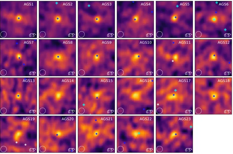
Fig. 7. ALMA 1.1 mm continuum maps for the 23 detections tapered at 0.60 arcsec. Each 300

5 × 300

5 image is centred on the position of the ALMA detection. Cyan double crosses show sources from the GOODS–S CANDELS catalogue. White circles show sources from the ZFOURGE catalogue. Blue circles show common sources from both optical catalogues (i.e. sources with an angular separation lower than 000

4). The shape of the synthesized beam is given in the bottom left corner.

2.0 1.5 1.0 0.5 0.0 0.5 1.0 1.5 2.0

["]

0.0

0.2

0.4

0.6

0.8

1.0

Flux (norm)

psf A

psf B

psf C

psf D

psf E

psf F

Fig. 8. East-West profile of the PSFs corresponding to the 6 different parallel slices composing the ALMA image in the 000

60-mosaic (see Fig.1).

The second test is to extract the flux for each galaxy using PSF-fitting. We use Galfit (Peng et al. 2010) on the 000 60-mosaic. The residuals of this PSF-extraction are shown for the 6 brightest galaxies in Fig.10. The residuals of 21/23 detections do not have a peak greater than 3 σ in a radius of 100_{around the}

source. Only sources AGS10 and AGS21 present a maximum in the residual map at ∼3.1 σ.

We compare the PSF flux extraction method with Gaussian and Sersic shapes. As our sources are not detected with a par-ticularly high SNR, and in order to limit the number of degrees of freedom, the Sersic index was frozen to n= 1 (exponential disk profile, in good agreement withHodge et al. 2016and El-baz et al. 2017for example), assuming that the dust emission is disk-like. Fig.10shows the residuals for the 3 different extrac-tion profiles. The residuals are very similar between the point source, Gaussian and Sersic profiles, suggesting that the approx-imation that the sources are not resolved is appropriate, and does not result in significant flux loss. We also note that, for several galaxies, due to large size uncertainties, the Gaussian and Sersic fits give worse residuals than the PSF fit (AGS4 for example).

For the third test, we take advantage of the different tapered maps. We compare the peak flux for each detection between the 00060-mosaic map and the 00029-mosaic map. The median ratio is S000₂₉

peak/S 000₆₀

peak= 0.87±0.16. This small decrease, of only 10% in the peak flux density between the two tapered maps suggests that the flux of the galaxies is only slightly more resolved in the 00029-mosaic map.

Having performed these tests, we conclude that these sources appear point-like at 0006 resolution. Our photometry is therefore performed under this assumption.

2.0 1.5 1.0 0.5 0.0 0.5 1.0 1.5 2.0

["]

0.0

0.2

0.4

0.6

0.8

1.0

Flux (norm)

stacked sources

stacked PSF

0.5 0.0 0.5

0"29

Fig. 9. Comparison between the stacked PSF (black solid line) and the stack of the 23 ALMA-detections (black dashed line) in the 000

60-mosaic. As each slice has a specific PSF, we stack the PSF correspond-ing to the position of each detection. The fluxes of each detection have been normalized, so that the brightest sources do not skew the results. Fluxes of the PSF and ALMA detections are normalized to 1. Flux profiles are taken across the East-West direction. The result is consis-tent with unresolved or marginally resolved sources at this resolution. The insert in the top-right corner shows the same procedure for the 15 sources detected in the 000

29-mosaic (see Table3).

5. Number counts 5.1. Completeness

We assess the accuracy of our catalogue by performing com-pleteness tests. The comcom-pleteness is the probability for a source to be detected in the map given factors such as the depth of the observations. We computed the completeness of our obser-vations using Monte Carlo simulations performed on the 000 60-mosaic map. We injected 50 artificial sources in each slice. Each source was convolved with the PSF and randomly injected on the dirty map tapered at 000_{60. In total, for each simulation run,} 300 sources with the same flux were injected into the total map. In view of the size of the map, the number of independent beams and the few number of sources detected in our survey, we can consider, to first order, that our dirty map can be used as a blank map containing only noise, and that the probability to inject a source exactly at the same place as a detected galaxy is negli-gible. The probability that at least two point sources, randomly injected, are located within the same beam (pb) is:

pb = 1 − k= n−1 Y k= 0 Nb− k Nb (3)

where Nbis the number of beams and n is the number of injected sources. For each one of the six slices of the survey, we count ∼100 000 independent beams. The probability of having source blending for 50 simulated sources in one map is ∼1%.

We then count the number of injected sources detected with σp= 4.8 σ and σf= 2.7 σ, corresponding to the thresholds of our main catalogue. We inject 300 artificial sources of a given flux, and repeat this procedure 100 times for each flux density. Our simulations cover the range Sν= 0.5-2.4 mJy in steps of 0.1 mJy. Considering the resolution of the survey, it would be reasonable to expect that a non-negligible number of galaxies are not seen as point sources but extended sources (see Sect.4.5). We sim-ulate different sizes of galaxies with Gaussian FWHM between 000_{2 and 0}00_{9 in steps of 0}00_{1, as well as point-source galaxies,}

to better understand the importance of the galaxy size in the de-tectability process. We match the recovered source with the input position within a radius of 000_6.

Fig. 11 shows the resulting completeness as a function of input flux, for different FWHM Gaussian sizes convolved by the PSF and injected into the map.

As a result of our simulations, we determine that at 1.2 mJy, our sample is 94±1% complete for point sources. This percent-age drastically decreases for larger galaxy sizes. For the same flux density, the median detection rate drops to 61±3% for a galaxy with FWHM ∼000_{3, and to 9±1% for a FWHM ∼0}00₆ galaxy. This means, that for a galaxy with an intrinsic flux den-sity of 1.2 mJy, we are more than ten times more likely to detect a point source galaxy than a galaxy with FWHM ∼0006.

The size of the millimetre emission area plays an essential role in the flux measurement and completeness evaluation. We took the hypothesis that ALMA sizes are 1.4 times smaller than the size measured in HST H-band (as derived byFujimoto et al. 2017using 1034 ALMA galaxies). We are aware that this size ratio is poorly constrained at the present time, but such relation has been observed in several studies (see Sect.4.5). For exam-ple, of the 12 galaxies presented byLaporte et al.(2017), with fluxes measured using ALMA at 1.1mm (González-López et al. 2017), 7 of them have a size measured by HST F140W/WFC3

similar to the size measured in the ALMA map. On the other hand, for the remaining 5 galaxies, their sizes are approximately two times more compact at millimetre wavelengths than at opti-cal wavelengths. This illustrates the dispersion of this ratio.

5.2. Effective area

As the sensitivity of our 1.1mm ALMA map is not uniform, we define an effective area where a source with a given flux can be detected with an SNR > 4.8 σ, as shown in Fig. 12. Our map is composed of 6 different slices - one of them, slice B, presents a noise 30% greater than the mean of the other 5, whose noise levels are comparable. The total survey area is 69.46 arcmin2_{, with 90% of the survey area reaching a sensitivity of at} least 1.06 mJy.beam−1. We consider the relevant effective area for each flux density in order to compute the number counts. We consider the total effective area over all slices in the number counts computation.

5.3. Flux Boosting and Eddington bias

In this section, we evaluate the effect of flux boosting. Galaxies detected with a relatively low SNR tend to be boosted by noise fluctuations (seeHogg & Turner 1998;Coppin et al. 2005;Scott et al. 2002). To estimate the effect of flux boosting, we use the same set of simulations that we used for completeness estima-tions.

The results of our simulations are shown in Fig. 13. The boosting effect is shown as the ratio between the input and out-put flux densities as a function of the measured SNR. For point sources, we observe the well-known flux boosting effect for the lowest SNRs. This effect is not negligible for the faintest sources in our survey. At 4.8 σ, the flux boosting is ∼15%, and drops below 10% for an SNR greater than 5.2. We estimate the de-boosted flux by dividing the measured flux by the median value of the boosting effect as a function of SNR (red line in Fig.13).

We also correct for the effects of the Eddington bias ( Edding-ton 1913). As sources with lower luminosities are more numer-ous than bright sources, Gaussian distributed noise gives rise to