HAL Id: pasteur-02076664
https://hal-pasteur.archives-ouvertes.fr/pasteur-02076664
Submitted on 22 Mar 2019
HAL is a multi-disciplinary open access
archive for the deposit and dissemination of
sci-entific research documents, whether they are
pub-lished or not. The documents may come from
teaching and research institutions in France or
abroad, or from public or private research centers.
L’archive ouverte pluridisciplinaire HAL, est
destinée au dépôt et à la diffusion de documents
scientifiques de niveau recherche, publiés ou non,
émanant des établissements d’enseignement et de
recherche français ou étrangers, des laboratoires
publics ou privés.
Distributed under a Creative Commons Attribution| 4.0 International License
Mining Tool for Unraveling the Complexity of Biological
Systems – Novel Insights into Malaria
Cheikh Loucoubar, Richard Paul, Avner Bar-Hen, Augustin Huret, Adama
Tall, Cheikh Sokhna, Jean-Francois Trape, Alioune Badara Ly, Joseph Faye,
Abdoulaye Badiane, et al.
To cite this version:
Cheikh Loucoubar, Richard Paul, Avner Bar-Hen, Augustin Huret, Adama Tall, et al.. An
Exhaus-tive, Non-Euclidean, Non-Parametric Data Mining Tool for Unraveling the Complexity of Biological
Systems – Novel Insights into Malaria. PLoS ONE, Public Library of Science, 2011, 6 (9), pp.e24085.
�10.1371/journal.pone.0024085�. �pasteur-02076664�
Mining Tool for Unraveling the Complexity of Biological
Systems – Novel Insights into Malaria
Cheikh Loucoubar1,2,3, Richard Paul1, Avner Bar-Hen2,4, Augustin Huret5, Adama Tall3, Cheikh Sokhna6,
Jean-Franc¸ois Trape6, Alioune Badara Ly3, Joseph Faye3, Abdoulaye Badiane3, Gaoussou Diakhaby3,
Fatoumata Die`ne Sarr3, Aliou Diop7, Anavaj Sakuntabhai1,8*, Jean-Franc¸ois Bureau1
1 Institut Pasteur, Unite´ de Pathoge´nie Virale, Paris, France, 2 Laboratoire de Mathe´matiques Applique´es Paris 5 (UMR 8145), Universite´ Paris Descartes, Paris, France, 3 Unite´ d’E´pide´miologie des Maladies Infectieuses (UR 172), Institut Pasteur de Dakar, Dakar, Se´ne´gal, 4 Ecole des Hautes Etudes en Sante´ Publique, Rennes, France, 5 Institute of Health and Science, Paris, France, 6 Unite´ de Paludologie Afro-Tropicale (UMR 198), Institut de Recherche pour le De´veloppement, Dakar, Se´ne´gal, 7 Laboratoire d’E´tudes et de Recherche en Statistique et De´veloppement, UGB, Saint-Louis, Se´ne´gal, 8 Center of Excellence for Vectors and Vector-Borne Diseases, Faculty of Science, Mahidol University, Bangkok, Thailand
Abstract
Complex, high-dimensional data sets pose significant analytical challenges in the post-genomic era. Such data sets are not exclusive to genetic analyses and are also pertinent to epidemiology. There has been considerable effort to develop hypothesis-free data mining and machine learning methodologies. However, current methodologies lack exhaustivity and general applicability. Here we use a novel non-parametric, non-euclidean data mining tool, HyperCubeH, to explore exhaustively a complex epidemiological malaria data set by searching for over density of events in m-dimensional space. Hotspots of over density correspond to strings of variables, rules, that determine, in this case, the occurrence of Plasmodium falciparum clinical malaria episodes. The data set contained 46,837 outcome events from 1,653 individuals and 34 explanatory variables. The best predictive rule contained 1,689 events from 148 individuals and was defined as: individuals present during 1992–2003, aged 1–5 years old, having hemoglobin AA, and having had previous Plasmodium malariae malaria parasite infection #10 times. These individuals had 3.71 times more P. falciparum clinical malaria episodes than the general population. We validated the rule in two different cohorts. We compared and contrasted the HyperCubeH rule with the rules using variables identified by both traditional statistical methods and non-parametric regression tree methods. In addition, we tried all possible sub-stratified quantitative variables. No other model with equal or greater representativity gave a higher Relative Risk. Although three of the four variables in the rule were intuitive, the effect of number of P. malariae episodes was not. HyperCubeH efficiently sub-stratified quantitative variables to optimize the rule and was able to identify interactions among the variables, tasks not easy to perform using standard data mining methods. Search of local over density in m-dimensional space, explained by easily interpretable rules, is thus seemingly ideal for generating hypotheses for large datasets to unravel the complexity inherent in biological systems.
Citation: Loucoubar C, Paul R, Bar-Hen A, Huret A, Tall A, et al. (2011) An Exhaustive, Non-Euclidean, Non-Parametric Data Mining Tool for Unraveling the Complexity of Biological Systems – Novel Insights into Malaria. PLoS ONE 6(9): e24085. doi:10.1371/journal.pone.0024085
Editor: Fabio T. M. Costa, State University of Campinas, Brazil
Received May 31, 2011; Accepted July 29, 2011; Published September 9, 2011
Copyright: ß 2011 Loucoubar et al. This is an open-access article distributed under the terms of the Creative Commons Attribution License, which permits unrestricted use, distribution, and reproduction in any medium, provided the original author and source are credited.
Funding: Funding was provided by Institut Pasteur and the Ecole des Hautes Etudes en Sante´ Publique. The funders had no role in study design, data collection and analysis, decision to publish, or preparation of the manuscript.
Competing Interests: The authors have declared that no competing interests exist. * E-mail: anavaj@pasteur.fr
Introduction
Identifying the key variables of a biological system that determine the outcome of interest is difficult. Not only are there potentially many factors involved, but they also do not work independently. Testing for all possible interactions is almost impossible both with respect to statistical validation and biological interpretation. There is a need for data mining tools to explore large and complex biological data sets to identify combinations of factors that optimally explain the outcome of interest. Hypothesis-free data exploration can potentially generate novel hypotheses that emerge from the data and which are beyond our imagination. These novel hypotheses can subsequently be tested using standard statistical methods.
To date, data mining tools have been primarily developed for data retrieval through search engines. In biology, this has been essentially focused on sequence alignment algorithms to manage the ever-increasing amount of genetic data. More recently, data mining technology has been proposed as an alternative to traditional statistics to deal with high dimensional data generated by Genome Wide Association studies, in the knowledge that accounting for gene-gene and gene-environment is crucial to understand human genetic susceptibility to disease [1,2,3,4]. In addition to such methods in the field of genetic data analyses, several new heuristic tools have been developed, notably non-parametric modeling techniques such as Classification And Regression Trees (CART) [5] and Random Forests [6]. These methods present several advantages: models have the capacity to
provide accurate fits of the response in a wide variety of situations, enabling fitting of non-linear relationships between explanatory variables and the dependant variable, with no assumption that explanatory variables are independent. CART is a rule-based method that generates a binary tree through recursive partitioning. This splits a subset (called a node) of the data set into two subsets (called sub-nodes) according to minimization of a heterogeneity criterion computed on the resulting sub-nodes. Random forests is a procedure that generates a large number of tree predictors and then selects the most popular class. Despite the analytical advances of all of these techniques, none perform exhaustive exploration of the data [4] and to date, there is no algorithm that can search for all possible stratifications and identify the best combination of variables to explain a specified outcome.
Complementary to these non-parametric methods and to traditional statistical methods, a new approach, HyperCubeH (Institute of Health & Science, Paris, France) is based on the latest research in artificial intelligence, using least general generalized algorithms and genetic algorithms. The underlying idea is to describe a dataset by a group of « local over densities » of a specific outcome with no a priori hypothesis or notion of distance, each « over density » being completely independent from every other. The breakthrough is the ability to deal with points in a space with absolutely no assumptions, including those concerning metric and distance or nature of neighborhood. Indeed, working with a distance or a defined topology is already an assumption and either is not true or introduces bias into the model.
This method has been applied to various topics, mainly in the financial and business sectors, but remains unvalidated in the field of biology [7]. Through exhaustive exploration of m-dimensional space, HyperCubeH will classify subsets of the study population into high and low risk groups and pinpoint not only the key explanatory variables and their interactions, but also the key range of values within each explanatory variable. Whilst this approach has evident value for risk factor analysis critical for clinical decision making, it also offers a tool with which to explore complexity, potentially revealing unimaginable combinations of explanatory variables underpinning the observed outcome.
We report here a rigorous assessment of the performance of this novel HyperCubeH method. The aim of the study is to test whether the rules identified by HyperCubeH give the best predictive value. We use HyperCubeH to explore a large longitudinal epidemiological data set of malaria. We compare the predictive value of the rules identified by HyperCubeH with models generated using classical statistical methods, binomial regression and CART. We demonstrate that HyperCubeH can identify the best combination of factors predicting the outcome of malaria infection in our dataset.
Results
Populations, outcome and explanatory variables
We studied a large dataset from a long-term epidemiological study of two family-based cohorts in Senegal, followed for 19 years (1990–2008) in Dielmo and for 16 years (1993–2008) in Ndiop [8,9]. Time period of observation was classified as a trimester. The dependant variable was defined as a binary trait: individuals with at least one clinical Plasmodium falciparum malaria attack (PFA) during that trimester or without PFA. In total, there were 46,837 outcome events of person-trimesters from 1,653 individuals. Almost 20% of the events were PFA in both villages. Thirty-four explanatory variables for association with the occurrence of PFA were considered. Twenty one variables were qualitative (eight nominal and 13 ordered) and 13 were quantitative (Table 1 and 2).
HyperCubeH analysis
We first analyzed the data using HyperCubeH. We divided our dataset into 3 phases: Learning, Validation and Replication. We analyzed the two cohorts separately. A random variable was created dividing the data of each cohort into two groups of equal size (in and out samples). The learning phase was carried out using the ‘‘in sample’’ from the first studied cohort. In the validation phase, rules defined in the learning phase were validated in the ‘‘out sample’’ of the same cohort. The learning set contained 11,893 events and the validation set had 11,939 in Dielmo, while in Ndiop there were 11,530 events in the learning set and 11,475 in the validation set. The effect of each validated rule from the first cohort was studied in the second cohort in the replication phase. We defined three parameters for running the learning process, ‘‘Lift’’, ‘‘Size’’ and ‘‘Complexity’’. ‘‘Lift’’ is the ratio of the prevalence of positive PFA events within a rule over the prevalence of positive PFA events in the entire population; this is equivalent to relative risk (RR). ‘‘Size’’ is the minimum number of events described by the rule. ‘‘Complexity’’ describes the maximum number of variables in a rule. Choice of ‘‘Lift’’ and ‘‘Size’’ parameters are optimized using the ‘‘Signal Intensity Graph’’ (see Material and Method). The ‘‘Complexity’’ parameter is here fixed to six factors, of which two are forced, the ‘‘in sample’’ and the cohort. Table 3 summarizes the parameters used and results obtained from the HyperCubeH analyses.
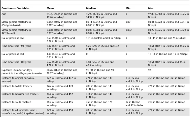
After 27 and 23 hours of analyses, we obtained 4,853 and 6,860 rules in Dielmo and Ndiop, respectively. We calculated the probability for the occurrence of a rule with identical ‘‘Lift’’ and ‘‘Size’’ parameters from randomization of the entire dataset to obtain an empirical P value (empP). We selected minimized rules (see materials and methods) with empP less than 10280in Dielmo and Ndiop, for the validation phase (Table 3). We used this high threshold empP for selection to minimize the risk of over-fitting. We were able to validate 51 of 52 minimized rules (98%) and 36 of 36 (100%) in Dielmo and Ndiop respectively. Of these, all 51 (100%) rules from Dielmo were replicated in Ndiop and all 36 (100%) rules from Ndiop were replicated in Dielmo with empP less than 1023. We selected the best predicted rule for further statistical study (Figure 1). The best predictive rule contained 1,689 events from 148 individuals and was defined as: individuals who lived in Dielmo during 1992 to 2003, were of an age between 1 to 5 years old, having hemoglobin type AA, and having had previous Plasmodium malariae infection (PMI) less than or equal to 10 times. These individuals had 3.71 (95%CI: 3.58–3.84) times more PFA than the general population; and this sub-population was the most representative (i.e. containing the maximum number of events) among those with a RR of at least equal to 3.71.
Confirmation of the HyperCubeH rule with traditional statistical methods
We sought to replicate the HyperCubeH rule using logistic regression. We redefined continuous variables as binary variables according to the HyperCubeH rule: The ‘‘Year’’ variable was defined as after 1991 and before 2004 or else; Age variable as between 1 and 5 years old or else; Hemoglobin type AA or else and cumulative number of previous PMIs as #10 times or else. By multivariate analysis, we tested all possible interactions between two variables and dropped interaction terms with P.0.05 until all had P#0.05. The variables showed highly significant marginal effect (P,0.0001) except age (Table 4). Age was highly significant (P,1024) when taking into account other criteria including year (between 1992 and 2003) and previous PMIs (#10). Analysis incorporating all possible interaction terms (i.e. with more than 2 variables) generated considerable over-dispersion and was difficult
to interpret. This result demonstrates that even though age is a major factor influencing development of PFA, without considering other variables, this effect would have been missed.
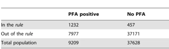
In order to replicate precisely the HyperCubeH rule and determine the relative risk for comparison with other models/ rules, we estimated the overall effect of the four key variables and all their possible interactions by defining a dummy variable X to represent the two sub groups of the population: X = 1 for a sub-population defined by the observations in the rule (i.e. living in Dielmo during 1992 to 2003, age 1 to 5 years old, having hemoglobin type ‘‘AA’’ and having had previous PMIs#10); X = 0, otherwise (Table 5). Table 5 shows 1,232 PFA+457 not PFA in the rule = 1,689 events via HyperCubeH. The Pearson chi-square test confirmed the strongly significant probability to develop PFA (x2 = 2740.55, DF = 1, P,10216), yielding a RR of 3.71 (95%CI: 3.58–3.84) and odds ratio (OR) of 11.02 (95%CI: 9.87–12.29). Using logistic regression, we confirmed the results of HyperCubeH.
Replication of the rule in the 2nd cohort
In order to validate the biological and epidemiological aspect of this HyperCubeH rule, it was replicated in Ndiop where a sub-population defined as above for Dielmo presented a higher risk to develop PFA compared to the general population: (x2 = 665.96, DF = 1, P,10216), RR of 2.35 (95%CI: 2.22–2.48) and OR of 3.50 (95%CI: 3.16–3.87). The result was optimal in Dielmo and replicated in Ndiop. The four variables identified above to be risk factors in Dielmo were thus also risk factors in Ndiop. Keeping the
same settings as in Dielmo for time period (from 1992 to 2003), previous PMIs (#10) and hemoglobin (‘‘AA’’), risk was maximum when age was re-set to 3 to 7 years old, with a RR of 2.53 (95%CI: 2.41–2.66) and OR of 4.04 (95%CI: 3.67–4.45) with more events (size = 1,761 events from 181 individuals) and more strongly significant (x2 = 933.93, DF = 1, P,10216) than when using the Dielmo age range of 1–5 years old (Size of 1,607 events from 158 individuals). This risk in Ndiop was, however, still lower than in Dielmo.
The two cohorts differ in one very pertinent manner: in Dielmo malaria transmission occurs all year round because of the presence of a small stream that enables mosquitoes to breed. In Ndiop, transmission is highly seasonal and occurs during the rainy season (July–December). Hence, we calculated the risk in Ndiop using only the period of year between July to December, a period when environmental factors are similar in the two villages. We obtained the same relative risk, RR = 3.78 (95%CI: 3.62–3.94), OR of 11.80 (95%CI: 10.11–13.77), with a highly significant Pearson chi-square test (x2 = 1542.50, DF = 1, P,10216). Furthermore, this risk was maximum when using age 3 to 7 years old (RR = 4.11, 95%CI: 3.97–4.27 and OR = 17.31, 95%CI: 14.68–20.41) with more events (Size = 932 events from 179 individuals vs. of Size of 863 from 157 when using age 1 to 5) and higher significance (x2 = 2076.17, DF = 1, P,10216).
Comparison with other models
We examined whether a classical statistical method could identify the same or better rules. We performed logistic regression Table 1. List of explanatory categorical variables.
Categorical (nominal) Variables No of levels
House 67 (36 in Dielmo and 31 in Ndiop) Independent Family 36 (12 in Dielmo and 24 in Ndiop)
Sex 2
Hemoglobin Type 7 (5 in Dielmo and 7 in Ndiop)
ABO blood group 4
G6PD Haplotype (on 4 SNPs: G6PD-376*, G6PD-202*, G6PD-968* and G6PD-542*) 11
PMI 2
POI 2
Categorical (ordered) Variables No of levels Drug treatment period 4
Year 19 (19 in Dielmo and 16 in Ndiop)
Trimester 4 ABO-261*: rs8176719 3 ABO-297*: rs8176720 3 ABO-467*: rs1053878 3 ABO-526*: rs7853989 3 ABO-771*: rs8176745 3 Alpha globin-3.7deletion 3 G6PD-202*: rs1050828 3 G6PD-376*: rs1050829 3 G6PD-542*: rs5030872 3 G6PD-968*: rs76723693 3
G6PD: Glucose-6-phosphate dehydrogenase, PMI: Plasmodium malariae infection, POI: Plasmodium ovale infection. *: Position on the gene.
analysis and CART using the Dielmo data. We first tested the effect of each variable on PFA by univariate analysis. When two or more variables were correlated, the most explicative variable was chosen. Continuous explanatory variables were categorized to enable comparison with HyperCubeH, by grouping the range of values having similar values for the dependant variable. Searching for the cut-off values for continuous variables was guided by Classification and Regression Trees (CART) methods [5]. CART identified cut-off values to categorize Age and Exposure variables, but did not find significant cut-off values for previous PMIs or any other continuous variable. Therefore, median was chosen as the cut-off value for each of these other variables. We then selected variables that showed #0.10 type I error for multivariate analysis (Table 6 and 7). As HyperCubeH dichotomizes any variable, being in or out of the rule; we redefined each variable in a similar way. Categorical, ordinal and interval variables that had more than 2 levels were redefined by regrouping levels for which their partial
effects were in the same direction. Trimester variable was redefined as semester (January–June and July–December) since the first two trimesters had decreasing effects and the last two had increasing effects on PFA when we adjusted on the other variables. Year variable was redefined in two levels (period 1: ‘‘year#2003’’ and period 2: ‘‘year$2004’’) according to the effect of each year. Age variable was classified into two levels (having between 0.4 and 8.1 years-old or else) according to CART analysis, ABO blood group in two levels (O or not O). Table 8 shows the result of univariate analysis after redefinition. For multivariate analysis we used the binary explanatory variables from Tables 6–8 and analyzed by logistic regression using several model selection methods: (1) selection based on an exhaustive screening of candidate models in each subset of explanatory variables, selecting the best one in terms of Information Criterion (lowest Akaike Information Criterion (AIC)); (2) forward selection and backward elimination. Model selection was computed using Package Table 2. List of explanatory continuous variables.
Continuous Variables Mean Median Min Max Age 21.35 (23.14 in Dielmo and
19.46 in Ndiop)
15.90 (17.06 in Dielmo and 14.97 in Ndiop)
0 97.88 (97.88 in Dielmo and 83.25 in Ndiop)
Mean genetic relatedness (Pedigree-based) 0.012 (0.012 in Dielmo and 0.012 in Ndiop) 0.011 (0.012 in Dielmo and 0.008 in Ndiop) 0.001 0.041 (0.028 in Dielmo and 0.041 in Ndiop)
Mean genetic relatedness IBD*-based) 0.008 (0.008 in Dielmo and 0.007 in Ndiop) 0.007 (0.008 in Dielmo and 0.007 in Ndiop) 0.002 0.029 (0.025 in Dielmo and 0.029 in Ndiop)
No. of previous PMI 2.53 (4.10 in Dielmo and 0.82 in Ndiop)
1 (1 in Dielmo and 0 in Ndiop) 0 44 (44 in Dielmo and 9 in Ndiop) Time since first PMI (year) 6.07 (6.67 in Dielmo and
5.03 in Ndiop)
5.25 (5.95 in Dielmo and4.32 in Ndiop)
0 18.51 (18.51 in Dielmo and 15.25 in Ndiop)
No. of previous POI 1.09 (1.33 in Dielmo and 0.83 in Ndiop)
0 0 11 (11 in Dielmo and 10 in Ndiop) Time since first POI (year) 5.52 (6.20 in Dielmo and
4.72 in Ndiop)
4.88 (5.55 in Dielmo and 4.25 in Ndiop)
0 18.51 (18.51 in Dielmo and 15 in Ndiop)
Exposure (number of days present in the village) per trimester
80.76 (81.65 in Dielmo and 79.87 in Ndiop)
91 (91 in Dielmo and 90 in Ndiop)
1 92
Distance to animal enclosure (meters) 322 in Dielmo and 147 in Ndiop 271 in Dielmo and 139 in Ndiop 1 in Dielmo and 2 in Ndiop
765 in Dielmo and 393 in Ndiop Distance to toilets (meters) 326 in Dielmo and 149
in Ndiop
280 in Dielmo and 143 in Ndiop
1 in Dielmo and 2 in Ndiop
774 in Dielmo and 401 in Ndiop Distance to house’s tree (meters) 344 in Dielmo and 152
in Ndiop
311 in Dielmo and 149 in Ndiop
1 in Dielmo and 1 in Ndiop
759 in Dielmo and 386 in Ndiop Distance to wells (meters) 365 in Dielmo and 195
in Ndiop
453 in Dielmo and 174 in Ndiop
17 in Dielmo and 17 in Ndiop
719 in Dielmo and 483 in Ndiop Distance to all (animals, toilets,
house’s tree, wells) together (meters)
329 in Dielmo and 150 in Ndiop 288 in Dielmo and 143 in Ndiop 1 in Dielmo and 1 in Ndiop
774 in Dielmo and 483 in Ndiop *IBD: Identity-By-Descent.
doi:10.1371/journal.pone.0024085.t002
Table 3. Parameters used and rules obtained from the HyperCubeH analyses.
Cohort Total number of events
Learning
Set Validation Set Purity Lift Size
Time of run Coverage Number of Totalrules Number of minimized rules Number of validated rules Number of replicated rules Dielmo 23,832 11,893 11,939 0.73 4.00 400 27 h 67% 4,853 52 51 51 Ndiop 23,005 11,530 11,475 0.74 3.49 400 23 h 72% 6,860 36 36 36 Purity: prevalence of events {PFA = 1} in the rule; Lift: Relative Risk of belonging to the rule compared to the total population; Size: number of events in the rule; Coverage: percentage of events {PFA = 1} in all rules found by HyperCubeH compared to the total number of events {PFA = 1} in the whole dataset.
‘‘glmulti’’ of R software [10]. The results obtained are presented in Table 9.
According to the results of the multivariate regression model selection (Table 9), we defined for each selected model a sub-group X = 1 when all risk factors are present, otherwise X = 0. For each model, we gave RR, p-value, and number of events for the sub-group
having all identified risk factors. All sub-groups identified using model selection techniques had lower predictive values for developing PFA than the HyperCubeH rule (Table 9). For sub-groups explaining the same or a greater number of events than the one found by HyperCubeH, the RR was lower and the 95% confidential intervals of RR did not overlap with those for the HyperCubeH rule (Table 9).
Figure 1. Typical result from HyperCubeH. A) Table ‘‘Key Indicators’’ shows Lift: 1.39; Size: 1,689; Purity: 0.73. B) Graph showing comparative proportion of events within the rule and events in the entire population, pink: affected (PFA positive), green unaffected (PFA negative). Both pink and green bars would reach the horizontal red line if there was same proportion of positive PFA in the rule and in the entire population. C) Table ‘‘Rule space’’ shows marginal contribution of each variable to the lift. Loss: gives partial decreases of lift when removing each variable (or risk factor) from the rule; Coverage: percentage of events {PFA = 1} defined by the corresponding variable alone compared to the total number of events {PFA = 1} in the whole dataset; Size: increase of events in a rule when the constraint defined within a variable is cancelled or by dropping the variable. D) Graphs showing distribution (in blue) of each variable, and the range of values (in green) within the rule.
doi:10.1371/journal.pone.0024085.g001
Table 4. Multivariate analysis of risk factors associated with clinical P. falciparum malaria attacks in Dielmo using the HyperCubeH rule.
Parameters DF Estimate SE x2 Pr.x2 OR Wald 95%CL Intercept 1 23.43 0.16 483.4 ,.0001 - - -Age group (years) 1 to 5 1 0.38 0.28 1.8 0.178 1.46 [0.84 2.53] Type of hemoglobin AA 1 0.38 0.07 27.8 ,.0001 1.46 [1.27 1.68] Year After 1991 and Before 2004 1 1.80 0.15 139.4 ,.0001 6.07 [4.50 8.19] Number of previous P. malariae infections #10 1 0.80 0.15 29.4 ,.0001 2.23 [1.67 2.97] Age group *P. malariae infections 1 to 5 #10 1 1.62 0.27 36.5 ,.0001 5.06 [2.99 8.56] Age group* Year 1 to 5 Before 2004 1 0.77 0.10 55.8 ,.0001 2.15 [1.76 2.63] P. malariae infections*Year #10 Before 2004 1 21.38 0.16 72.2 ,.0001 0.25 [0.18 0.35] DF: degree of freedom; Estimate: effect of explanatory variable’s levels on logit(Probability of {PFA = 1}); SE: standard error; x2: chi-square DF = 1; OR: Odds ratio; CL: confidential level.
We tested whether the HyperCubeH rule predicted the highest risk of developing PFA. We used the HyperCubeH model as a reference. We modified the reference HyperCubeH rule by either removing one of the variables or adding in variables identified by multivariate analysis. Using the same method to define subsets of the population and construct contingency tables, we calculated RR, OR and P values for each model. As shown in Table 10, there
was no other model that gave higher RR and/or OR than the one identified by HyperCubeH with equal or greater size.
In contrast to the regression analyses, CART found that age (between 0.22 and 5.48) and year (from 1990 to 2003) defined the high risk group for having PFA (RR = 3.26 [95CI: 3.16–3.38], OR = 7.34 [95CI: 6.80–7.93] and size = 3,041 with x2 = 3268.85, DF = 1 [P,10216]) (Figure 2). No other variable or combination of variables yielded a higher Relative Risk.
Optimality of HyperCubeH choice
We then tested whether the cut-off values delimiting the range of values in the HyperCubeH rule (defined as the reference rule) for each variable were the optimal ones. Hemoglobin type was fixed as AA or not. We modified the range of continuous variables of the reference rule. As the cut-off values for continuous variables were considered at integer values, there were a finite number of subsets that we could try for modifying a rule. We tested all possible ranges of the continuous variables (Age, previous PMIs and Year) with constraint of minimum ‘‘Size’’ of $400 events in the rules. We first fixed 2 variables and changed one variable at a time. The variable to change was first defined as the range of integer values Table 5. Number of positive/negative PFA events (P.
falciparum malaria attacks) in subgroups of individuals in and out of the HyperCubeH rule.
PFA positive No PFA In the rule 1232 457 Out of the rule 7977 37171 Total population 9209 37628 doi:10.1371/journal.pone.0024085.t005
Table 6. Univariate logistic regression analysis of each categorical risk factor for clinical falciparum malaria (PFA) attacks in Dielmo.
No of Person-trimesters N = 23832
PFA = 0 PFA = 1 Estimate(Std. Error) Crude OR Wald 95%CL P-values GlobalP N(%) = 19475 N (%) = 4357
Age group (years) [0–0.4] 303 (84.17) 57 (15.83) Ref. 1
[0.4–6.7] 2344 (46.72) 2673 (53.28) 1.80 (0.15) 6.06 [4.54–8.09] ,.0001
[6.7–8.12] 692 (67.13) 338 (32.82) 0.95 (0.16) 2.6 [1.9–3.55] ,.0001 ,.0001 [8.12–13.6] 2943 (81.28) 678 (18.72) 0.20 (0.15) 1.22 [0.91–1.65] 0.1782
$13.6 13138 (95.58) 608 4.42) 21.40 (0.15) 0.25 [0.18–0.33] ,.0001 Missing data 55 3 - - - -Sex Male 9663 (80.77) 2301 (19.23) Ref. 1
Female 9812 (82.68) 2056 (17.32) 20.13 (0.03) 0.88 [0.82–0.94] - ,.0001 Blood group O 7597 (79.56) 1952 (20.44) Ref. 1
A 5131 (83.65) 1003 (16.35) 20.27 (0.04) 0.76 [0.70–0.83] ,.0001
AB 920 (90.20) 100 (9.80) 20.86 (0.11) 0.42 [0.34–0.52] ,.0001 ,.0001 B 4496 (82.40) 960 (17.60) 20.19 (0.04) 0.83 [0.76–0.91] ,.0001
Missing data 1331 342 - - - -Type of hemoglobin AA 16304 (81.28) 3756 (18.72) Ref. 1
AC/AS/SS 2007 (87.53) 286 (12.47) 20.48 (0.07) 0.62 [0.54–0.70] ,.0001 Missing data 5196 1438 - - -
-G6PD Normal alleles 6448 (84.0) 1228 (16.0) Ref. 1
Mutated allele 7865 (82.30) 1691 (17.70) 20.12 (0.04) 0.89 [0.82–0.96] 0.0032 Missing data 5162 1438 - - -
-P. malariae infections #1 (median) 9348 (81.99) 2099 (18.34) Ref. 1
.1 8983 (79.91) 2258 (20.09) 0.11 (0.03) 1.12 [1.04–1.20] - 0.0008 missing 1144 0 - -
-P. ovale infections #0 (median) 9946 (81.54) 2251 (18.46) Ref. 1
.0 8385 (79.93) 2106 (20.07) 0.10 (0.03) 1.11 [1.04–1.19] - 0.002 missing 1144 0 - -
-Estimate: effect of explanatory variable’s levels on logit(Probability of {PFA = 1}); SE: standard error; OR: Odds ratio; CL: confidential level; Ref.: reference level. Age and Exposure were categorized using CART and previous PMIs and previous POIs using median since CART did not find significant cut-off values. doi:10.1371/journal.pone.0024085.t006
between its minimum and maximum values, and then reduced from the maximum to smaller integer values covering an ever-decreasing total age range until the minimum. This was repeated step by step until each integer value of the variable was set as the minimum for a step. Therefore, the total number of choices for a variable is 1+2+3+…+maximum = sum of a finite arithmetic sequence = (first value+last value)*(number of values)*(1/2). Each choice corre-sponds to a specific modification of the reference rule (i.e. a specific interval of values defining the modified rule). Then, for Age, previous PMIs and Year, there are (1+98)*98*0.5 = 4851, (1+45)*45*0.5 = 1035 and (1+19)*19*0.5 = 190 possible choices respectively. We then fixed 1 variable and changed 2 variables simultaneously. When Year is fixed and the couple (Age, previous PMIs) changed simultaneously, there are 4851*1035 = 5,020,785 possible choices. For previous PMIs fixed and (Age, Year) changed and Age fixed and (previous PMIs, Year) changed there are 4851*190 = 921,690 and 1035*190 = 196,650 possible choices. When we selected choices with at least same size as the reference rule, the resulting RR was always lower than the reference RR.
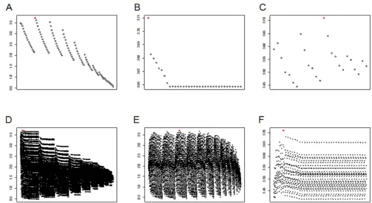
Figure 3 shows the effects of the modified ranges (i.e. the effect of other choices different from the one found by HyperCubeH) on RR. If all 3 variables were allowed to vary simultaneously there would be 4,851(Age) *190(Year) *1035(previous PMIs) = 953,949,150 possi-ble choices. The time for running such an analysis on one computer with 2 central processor units (Duo CPU 2.00 GHz 2.00 GHz), Memory (RAM) of 3.00 GB) is estimated at ,5678 days (,1.94 choices analyzed per second) using function ‘‘system.time(.)’’ of R-software, and thus not possible to analyze.
Discussion
We describe here a new data mining algorithm that can identify the combinations of variables that give the optimal prediction of the outcome of interest. We demonstrate that the model identified by HyperCubeH has better predictive value than any other model tested. HyperCubeH was able to identify the best cut-off value and range for continuous variables. It classified the population into high and low risk groups and made the results easier to interpret in Table 7. Univariate logistic regression analysis of each temporal risk factor for clinical falciparum malaria (PFA) attacks in Dielmo.
No of Person-trimesters N = 23832
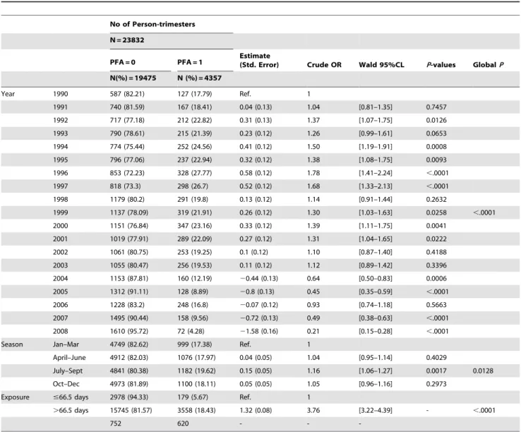
PFA = 0 PFA = 1 Estimate(Std. Error) Crude OR Wald 95%CL P-values GlobalP N(%) = 19475 N (%) = 4357 Year 1990 587 (82.21) 127 (17.79) Ref. 1 1991 740 (81.59) 167 (18.41) 0.04 (0.13) 1.04 [0.81–1.35] 0.7457 1992 717 (77.18) 212 (22.82) 0.31 (0.13) 1.37 [1.07–1.75] 0.0126 1993 790 (78.61) 215 (21.39) 0.23 (0.12) 1.26 [0.99–1.61] 0.0653 1994 774 (75.44) 252 (24.56) 0.41 (0.12) 1.50 [1.19–1.91] 0.0008 1995 796 (77.06) 237 (22.94) 0.32 (0.12) 1.38 [1.08–1.75] 0.0093 1996 853 (72.23) 328 (27.77) 0.58 (0.12) 1.78 [1.41–2.24] ,.0001 1997 818 (73.3) 298 (26.7) 0.52 (0.12) 1.68 [1.33–2.13] ,.0001 1998 1179 (80.2) 291 (19.8) 0.13 (0.12) 1.14 [0.91–1.44] 0.2632 1999 1137 (78.09) 319 (21.91) 0.26 (0.12) 1.30 [1.03–1.63] 0.0258 ,.0001 2000 1151 (76.84) 347 (23.16) 0.33 (0.12) 1.39 [1.11–1.75] 0.0041 2001 1019 (77.91) 289 (22.09) 0.27 (0.12) 1.31 [1.04–1.65] 0.0222 2002 1061 (80.75) 253 (19.25) 0.1 (0.12) 1.10 [0.87–1.40] 0.4188 2003 1055 (80.47) 256 (19.53) 0.11 (0.12) 1.12 [0.89–1.42] 0.3396 2004 1153 (87.81) 160 (12.19) 20.44 (0.13) 0.64 [0.50–0.83] 0.0006 2005 1312 (91.11) 128 (8.89) 20.8 (0.13) 0.45 [0.35–0.59] ,.0001 2006 1228 (83.2) 248 (16.8) 20.07 (0.12) 0.93 [0.74–1.18] 0.5663 2007 1495 (90.44) 158 (9.56) 20.72 (0.13) 0.49 [0.38–0.63] ,.0001 2008 1610 (95.72) 72 (4.28) 21.58 (0.16) 0.21 [0.15–0.28] ,.0001 Season Jan–Mar 4749 (82.62) 999 (17.38) Ref. 1
April–June 4912 (82.03) 1076 (17.97) 0.04 (0.05) 1.04 [0.95–1.14] 0.4029
July–Sept 4841 (80.38) 1182 (19.62) 0.15 (0.05) 1.16 [1.06–1.27] 0.0017 0.0128 Oct–Dec 4973 (81.89) 1100 (18.11) 0.05 (0.05) 1.05 [0.96–1.16] 0.2973
Exposure #66.5 days 2978 (94.33) 179 (5.67) Ref. 1
.66.5 days 15745 (81.57) 3558 (18.43) 1.32 (0.08) 3.76 [3.22–4.39] - ,.0001
752 620 - -
-Estimate: effect of explanatory variable’s levels on logit(Probability of {PFA = 1}); SE: standard error; OR: Odds ratio; CL: confidential level; Ref.: reference level. Age and Exposure were categorized using CART and previous PMIs and previous POIs using median since CART did not find significant cut-off values. doi:10.1371/journal.pone.0024085.t007
terms of biology than the probability estimates generated by most statistical methods.
The principle of this method is to explore all possible combinations of predictor variables and to find, through stochastic parallel computing exploration, the optimal hypercubes (or sub-spaces) defined by a combination of these variables, without making any assumptions. This method allows generation of rules, sets of variables and ranges of variable values that define subpopulations with high risk for the outcome of interest and that best predict the outcome. Inspired from latest research in artificial intelligence, Least General Generalized algorithms and Genetic Algorithms, HyperCubeH SaaS software generates local hypercubes and stabilizes each local hypercube to a local optimum, each optimum being new and independent. By doing so, it is possible to describe and understand local configurations without there being necessarily any global effect, i.e. some specific combination of factors that are only found in a sub-set of the population may increase the risk of outcome for that sub-population, but which are not detectable when averaged across the entire population. HyperCubeH enables us to describe the range of values and the combination of variables that can trigger the events. Although the statistics aims to reject, or not, a predefined assumption according to given risks, these complex event intelligence techniques allow us to generate assumptions on rules without any prerequisite. A hypercube is expressed in a simple formal way as a rule, directly readable and comprehensible.
As correction for multiple testing is not possible when using HyperCubeH, statistical validation and replication in independent cohorts are crucial, even prior to biological validation. We randomly divided the population in one cohort into the learning set and the validation set. We used the other cohort for replication. In addition, we calculated an empirical P value from whole randomized data. We demonstrated that using a high threshold of empirical P value (10280), 98–100% of the rules could be validated and 100% of validated rules could be replicated in another cohort despite their differences in human ethnicity and malaria endemicity [11].
Biological validation of the rule is most important. Here three of the variables are known a priori to increase the risk of developing
PFA: young children (i.e. lack of clinical immunity), normal hemoglobin Hb AA, and living during a period of intense malaria transmission. However, HyperCubeH allowed us to identify the range of continuous variables, such as age and year, which enable us to define high and low risk groups. In addition, the effect of these three variables alone did not reach our stringent acceptance threshold. Identifying an additional variable using classical techniques would be a big challenge due to the number of possible choices. HyperCubeH added a fourth one ‘‘number of previous PMIs at ranges less than or equal to 10’’ to define a rule containing 1,232 events with PFA and 457 events without PFA (prevalence = 72.9%) compared to 19.7% prevalence of the whole population (RR 3.71 (95%CI: 3.58–3.84). This RR is the highest of all models containing this number of events. This rule explained 28.28% of total events with PFA in the dataset.
The effect size of each variable was estimated by removing each variable and calculating the loss in ‘‘Lift’’ (Figure 1c). The strongest effect is age (68%), then village (18%), followed by year (7.3%). Hemoglobin type explained 3% of the ‘‘Lift’’ while previous PMIs had only 1.6% effect. There was 1.8% of the ‘‘Lift’’ that could not be explained by each of these variables individually (Table 11) and thus reflects interaction among the variables. In Dielmo, malaria transmission is holoendemic with an average of more than 200 infectious bites per person per year, 10 times more than Ndiop [12]. Therefore, individuals living in Dielmo have more chance to develop PFA. Age is a well known factor of PFA due to rapid development of clinical immunity in high malaria transmission regions. Using variance component analysis, age explained 29.8% of total variation in number of PFA in Dielmo [11]. The year effect is almost certainly yearly variation in transmission intensity. Indeed in 2003, the HyperCubeH rule threshold for year, a new drug for PFA treatment was introduced and malaria transmission decreased in following years. Hemoglo-bin type is one of the best known genetic factors protecting against malaria. In our and other studies, sickle cell mutation explained 2– 5% of risk in development of severe and clinical falciparum malaria [13], similar to that estimated by HyperCubeH (Table 11). The new variable that HyperCubeH identified is previous P. malariae Table 8. Univariate analysis of each risk factor (redefined in only two levels) for clinical P. falciparum malaria attacks (PFA) in Dielmo.
No of Person-trimesters N = 23832
PFA = 0 PFA = 1 Estimate (Std. Error) Crude OR Wald 95%CL P-values N (%) = 19475 N (%) = 4357
(81.72) (18.28)
Age group (years) ,0.4 or $8.12 16384 (92.42) 1343 (7.58) Ref. 1
[0.4–8.12] 3036 (50.21) 3011 (49.79) 2.49 (0.04) 12.1 [11.22–13.04] ,.0001 Missing data 55 3 - -
-Blood group A or B or AB 10547 (83.64) 2063 (16.36) Ref. 1
O 7597 (79.56) 1952 (20.44) 0.27 (0.04) 1.31 [1.23–1.41] ,.0001 Missing data 1331 342 - -
-Year $2004 6798 (89.87) 766 (10.13) Ref. 1
,2004 12677 (77.93) 3591 (22.07) 0.92 (0.04) 2.51 [2.31–2.73] ,.0001 Semester Jan–Jun 9661 (82.32) 2075 (17.68) Ref. 1
Jul–Dec 9814 (81.13) 2282 (18.87) 0.08 (0.03) 1.08 [1.16–1.16] 0.0179 Estimate: effect of explanatory variable’s levels on logit(Probability of {PFA = 1}); SE: standard error; OR: Odds ratio; CL: confidential level; Ref.: reference level. doi:10.1371/journal.pone.0024085.t008
Table 9. Multivariate model selection for risk factors associated with clinical P. falciparum malaria attacks (PFA) in Dielmo using factors identified from univariate logistic analysis. Best model (with lowest A IC) when number of explanatory variables is equal to: V a ri a b le s 1 2 3 456789 1 0 F o rw a rd * Backward* Sex F emale ! NSE 1 Age group (years) 0.4 to 8.1 ! ! ! !!!!!! ! 1N S R Blood Type O !! 9N S R Type o f h emoglobin A A !!! ! 7N S R G6PD Normal !!!!! ! 6N S R Year Before 2004 ! ! !!!!!! ! 2N S R Semester Jul–Dec !! ! 8N S R Exposure . 66.5 !!!!!! ! 4N S R P.malariae infections # 1 ! !!!!!! ! 3N S R P.ovale infections # 0 !!!! ! 5N S R RR 2.53 2.96 3.22 3.22 3.15 2.98 3.08 3.27 3.32 2.95 3.32 3.32 (95% C I) (2.45–2.61) (2.86–3.05) (3.10–3.35) (3.09–3.37) (2.93–3.38) (2.71–3.27) (2.79–3.40) (2.89–3.70) (2.83–3.91) (2.18–3.99) (2.83–3.91 ) (2.83–3.91) p-value , .0001 , .0001 , .0001 , .0001 , .0001 , .0001 , .0001 , .0001 , .0001 , .0001 , .0001 , .0001 Size of subset defined by all risk factors 6044 4277 2000 1520 5 07 316 2 61 143 7 8 3 1 7 8 7 8 ! : F or selected variables. NSE: N o (additional) effects met the 0.05 significance level for entry into the model. NSR: N o (additional) effects met the 0 .05 significance level for removal from the model. *: Both F orward and B ackward methods selected the best (in terms o f A IC) model w ith 9 explanatory variables. doi:10.1371/journal.p one.0024085.t009
Table 10. Predictive values of modified HyperCubeH rule.
Variable Size RR 95%CL OR 95%CL x2
DF Pr.x2
M.ref: 3.71 3.58 3.84 11.02 9.87 12.29 2741 1 ,.0001 P. malariae infections+Year+Age+Hemoglobin 1689
M.ref2P. malariae infections 1752 3.65 3.52 3.77 10.35 9.30 11.51 2705 1 ,.0001 M.ref2Year 2197 3.44 3.33 3.56 8.58 7.82 9.40 2843 1 ,.0001 M.ref2Age 10824 1.18 1.14 1.23 1.24 1.18 1.30 71 1 ,.0001 M.ref2Hemoglobin 1957 3.60 3.48 3.73 9.94 9.00 10.99 2898 1 ,.0001 M.ref+Sex2P. malariae infections 879 3.69 3.53 3.86 10.82 9.31 12.57 1475 1 ,.0001 M.ref+Sex2Year 1031 3.59 3.44 3.75 9.82 8.57 11.25 1592 1 ,.0001 M.ref+Sex2Age 5377 1.16 1.10 1.22 1.20 1.13 1.29 29 1 ,.0001 M.ref+Sex2Hemoglobin 990 3.62 3.46 3.78 10.06 8.75 11.56 1562 1 ,.0001 M.ref+Blood Type2P. malariae infections 784 3.61 3.44 3.79 10.03 8.58 11.72 1249 1 ,.0001 M.ref+Blood Type2Year 966 3.46 3.30 3.63 8.69 7.57 9.96 1351 1 ,.0001 M.ref+Blood Type2Age 4312 1.29 1.22 1.36 1.38 1.29 1.49 78 1 ,.0001 M.ref+Blood Type2Hemoglobin 852 3.66 3.50 3.83 10.48 9.01 12.19 1399 1 ,.0001 M.ref+G6PD2P. malariae infections 651 3.76 3.58 3.95 11.56 9.69 13.79 1162 1 ,.0001 M.ref+G6PD2Year 717 3.72 3.55 3.91 11.17 9.46 13.20 1244 1 ,.0001 M.ref+G6PD2Age 4840 1.17 1.11 1.23 1.22 1.13 1.31 30 1 ,.0001 M.ref+G6PD2Hemoglobin 661 3.84 3.66 4.02 12.59 10.53 15.05 1249 1 ,.0001 M.ref+Semester2P. malariae infections 884 3.77 3.62 3.94 11.76 10.09 13.69 1574 1 ,.0001 M.ref+Semester2Year 1117 3.56 3.41 3.72 9.54 8.38 10.86 1677 1 ,.0001 M.ref+Semester2Age 5458 1.23 1.17 1.30 1.31 1.23 1.40 64 1 ,.0001 M.ref+Semester2Hemoglobin 988 3.76 3.61 3.92 11.62 10.06 13.42 1734 1 ,.0001 M.ref+Exposure2P. malariae infections 1403 3.66 3.25 3.80 10.46 9.29 11.78 2228 1 ,.0001 M.ref+Exposure2Year 1804 3.44 3.31 3.57 8.51 7.69 9.42 2367 1 ,.0001 M.ref+Exposure2Age 8729 1.15 1.11 1.20 1.20 1.14 1.27 42 1 ,.0001 M.ref+Exposure2Hemoglobin 1535 3.62 3.49 3.76 10.14 9.05 11.35 2361 1 ,.0001 M.ref+P. ovale infections2P. malariae infections 729 3.88 3.71 4.06 13.13 11.06 15.60 1410 1 ,.0001 M.ref+P. ovale infections2Year 759 3.87 3.71 4.05 13.05 11.02 15.44 1459 1 ,.0001 M.ref+P. ovale infections2Age 4256 1.52 1.44 1.59 1.73 1.62 1.86 246 1 ,.0001 M.ref+P. ovale infections2Hemoglobin 768 3.85 3.69 4.03 12.79 10.82 15.10 1456 1 ,.0001 M.ref: reference model; Size: number of events; RR: risk ratio; OR: Odds ratio; x2: chi-square DF = 1; CL: confidential level.
doi:10.1371/journal.pone.0024085.t010
Figure 2. Decision tree generated by Classification and Regression Tree (CART) analysis of risk factors determining the occurrence ofP. falciparummalaria attacks (PFA) per trimester. Figure shows the cut-off values identified by CART that divide the dataset into two. At each leaf are given the Relative Risk (RR) and the number of events associated with that leaf.
infection - PMI. Although CART did not identify any significant threshold for previous PMI, using the median as the cut-off value gave a significant effect for previous PMI is the univariate logistic regression, whereby above median previous PMI increased risk of PFA (P = 0.0008, Table 6). Interestingly in the HyperCubeH rule the reverse was found and this is because of the interaction of
previous PMI with age: being young and having previous PMI decreased risk.
Cross-species immunity among different Plasmodium species has long been suspected and there is evidence of among-species negative interactions during concomitant infection [14,15]. An influence of P. malariae carriage on subsequent P. falciparum infection has been observed before. In Gabon, children infected with P. malariae presented more often with a P. falciparum infection and at higher parasite densities [16]. During the follow-up, subjects who were infected by P. malariae were reinfected by P. falciparum more rapidly. Such a relationship was also observed in the Garki project [15,17,18]. Although small scale variation in mosquito biting rate could generate similar levels of exposure to each parasite spp., the species infection association was found to be related to differences in acquired immunity and not to differences in exposure, suggesting that the levels of immunity to P. falciparum and to P. malariae were inter-related [18]. More recently, a family-based study found a strong relationship between P. falciparum parasite density and frequency of P. malariae infections [19]. P. falciparum parasite density has previously been shown to be under human genetic control and linked to the chromosomal region 5q31 in four independent studies [11,20,21,22]. These results suggest that individuals genetically susceptible to P. falciparum are also genetically pre-disposed to P. malariae [19]. Little is known on the impact of infection by one species on the incidence of disease of another. The relationships between parasite density and risk of attributable disease were found to be similar for P. falciparum, P. vivax and P. malariae in Papua New Guinea, compatible with the Table 11. Effect size of each variable in the rule.
DIELMO NDIOP
All year July December Loss % Loss Loss % Loss Loss % Loss Initial Lift 3.71 100% 2.35 100% 3.78 100% Age 22.53 268.2% 20.82 234.9% 21.26 233.3% Village 20.67 218.1% 20.7 229.8% 0.05 1.3% Year 20.27 27.3% 20.07 23.0% 20.06 21.6% Hb 20.11 23.0% 27.0% 23.0% 20.09 22.4% Previous PMIs 20.06 21.6% 20.13 25.5% 20.12 23.2% Semester - - - - 21.43 237.8% Total Loss 23.64 298% 21.79 276% 22.91 277% Residual Lift 0.07 1.9% 0.56 23.8% 0.87 23.0% Loss: partial decreases of lift when removing each variable from the rule. doi:10.1371/journal.pone.0024085.t011
Figure 3. Effect on relative risk (RR) of modifying the ranges of continuous variables. Graphs show RR for all other possible definitions of risk group on the explanatory variables, with equal or greater size than the HyperCubeH rule. Y-axis indicates the RR. A) Only ranges of Age are modified: 102 choices among 4,851 possible choices had size equal or greater than 1,689 (size of the HyperCubeH rule) and are plotted; B) Only ranges of previous PMIs are modified: 35 choices among 1,035 possible; C) Only ranges of Year are modified: 25 choices among 190 possible; D) Ranges of both Age and previous PMIs are modified simultaneously: 25,040 choices among 5,020,785 possible; E) Ranges of both Age and Year are modified simultaneously: 8,912 choices among 921,690 possible; F) Ranges of both previous PMIs and Year are modified simultaneously: 1,110 choices among 196,650 possible. Filled red triangle represents the RR of HyperCubeH’s rule (HyperCubeH’s risk group), empty black circles represent the RR of other choices of risk groups.
hypothesis that pan-specific mechanisms may regulate tolerance to different Plasmodium spp. [23]. Pertinent to our finding here, Black et al. found that children with symptomatic episodes not only presented with fewer mixed species infections, but also had fewer previous P. malariae infections than symptom-free children, as demonstrated by serology [24]. The induced infection experiments also provide evidence of the development of some cross-protective immunity [25]. Interestingly, previous infection with P. malariae has been previously shown to impact upon a P. falciparum infection, but with respect to the production of transmission stages and not clinical presentation [26,27].
Many other rules used this variable confirming that previous infection by P. malariae is associated with protection against development of PFA. It is presently impossible to conclude if this association is a causal one or is due to a correlation to an unknown factor affecting the risk to develop PFA. As both parasites are transmitted by the same mosquito species, increased exposure to one species (P. malariae) might be expected to correlate with increased exposure to the other (P. falciparum). Hence, spatial heterogeneity in the exposure to infection could simultaneously result in increase risk of infection by both parasite spp. Our analysis did not take into account ‘‘number of previous P. falciparum attacks’’ (nbpPFA) and so it is possible that the variable previous PMIs replaces this information. However, in another HyperCubeH analysis, we found that both previous PMIs and nbpPFA are used in different rules (data not shown), indicating that the previous infection by the two parasite species is not perfectly correlated. Thus, it seems probable that the parasite species effect reflects some impact of P. malariae infection on the development of immunity against P. falciparum. In our study, there were from 0 to 44 P. malariae infections per person prior to a clinical P. falciparum episode. HypercubeH identified that having few P. malariae infections (less than 10) was a potent risk factor, which excluded about 10% of events from those individuals who were often infected with P. malariae. The fact that a threshold of ten infections was identified as eliminating this risk factor is clearly not an exact threshold, but generally reflects the weakly immunising effect of P. malariae infection, reminiscent of that induced by P. falciparum infection. Furthermore, whereas eighteen out of 51 rules used the number of previous P. malariae infections, none used the number of previous P. ovale infections, illustrating that infection by the two Plasmodium species differently affects susceptibility to P. falciparum attacks. However, it should be noted that the absence of an effect of P. ovale on clinical P. falciparum attacks does not mean that P. ovale definitively has no effect. It may be the case that additional variables may be required to be taken into account. Indeed, in the multivariate model selection analysis (Table 9), previous P. ovale infection is significantly as a risk factor when a minimum of 6 explanatory variables are used. In our HyperCubeH analyses, we limited the number of variables in a single rule to four. This differential species effect is currently under investigation.
We compared the rule with the model identified by classical logistic regression method. Although we aimed to include all possible interaction terms among variables studied in multivariate analysis, over-dispersion of the data made this unstable. In addition, the running time would have been unacceptably long, taking ,5678 days for one a common computer to analyze about 109 models (3 variables with around 103 cases for each). With HyperCubeH, it took 23 to 27 hours to analyze 35 variables. In addition, the results of testing interaction among more than 2 variables by classical methods are difficult to interpret. We demonstrated that by omitting or adding other variables identified by other statistical methods or varying the cut-off value of continuous variables, the rule still performed best. Although some
rules had higher RR, they have lower ‘‘Size’’ or more complexity and less significant P value. Among rules with ‘‘Size’’ equal to or greater than 1,689, the same as the reference rule, the reference rule gave the highest RR.
Interestingly, the rule identified by classical method covered 0.67% of total positive events whereas one HyperCubeH rule explained 13.4%. When considering the minimized rules, we could identify risk factors that could explain 67% of total positive events, a percentage of coverage that would never be achieved by classical methods. While the classical method looked at events in 2 dimensions, HyperCubeH identified rules in multi-dimensional space. Although all factors identified by the classical method are risk factors for development of PFA, different groups of people developed PFA for different reasons. The rule identified by the classical method involved only individuals who had all the risk factors. We could only separate groups of individuals with different risk factors when looking at the events in multi-dimensional space. Analysis by CART identified a combination of variables, Age and Year, that increased risk of PFA. Both of these variables and the range of these variables were very similar to those identified by HyperCubeH. That CART failed to detect Hemoglobin or previous PMIs likely reflects the differences in methodologies of the two techniques. CART uses a sequential approach first splitting the data set according to the most significant variable and identifying the threshold value of that variable that maximizes the discrimination in the two subsets of data (i.e. least PFA vs. most PFA). Then, CART will further sub-divide each subset by the next most significant variable that leads to maximum discrimination. This approach thus leads to canalization of the data along different pathways, resulting in a decreased sample size for comparison. In addition, optimization by maximum discrimination at each level may paradoxically lead to an erroneous sub-optimal end-point many levels down. HyperCubeH, by contrast, analyses all variables simultaneously with no sequential selection that leads to such loss of power or canalization along a potentially eventual sub-optimal pathway.
One limitation arises when studying qualitative variables with more than two levels. It is not possible for HyperCubeH to combine levels having a similar effect in the same rule. One alternative would be to use analysis of variance, as we previously did in our classical analysis for qualitative variables with more than 2 levels, to detect modalities having a similar effect on the dependant variable and group them a priori.
Another more practical problem comes from the efficiency of the learning process. This process is more efficient in explaining the minor outcome, which is sometimes not the standard way of thinking. For instance, we could identify only factors increasing the risk of PFA, but not those conferring protection against malaria, which is the classical choice in malaria field. The positive events for PFA made up ,15% of the total number of events. To identify factors conferring protection (negative PFA), of which the prevalence was 85%, would have presented a vastly increased analytical challenge and yielded many, many more rules.
The choice of minimum group size for the outcome variable can, however, generate problems for biological interpretation. For example, here we observe that hemoglobin AA (normal hemoglo-bin) increases risk for development of PFA compared to the mutated sickle form, AS, which is known to confer protection. Importantly, we cannot conclude from our analysis that AS confers protection. In general, care must be taken in interpreting the direction of the effect and further specific analyses should be performed prior to establishing formal conclusions.
Repeated measures and potential pseudo-replication of events from the same individual are difficult to take into account. Whilst
this can be accounted for a posteriori in confirmatory classical analyses, this cannot be currently taken into account in HyperCubeH. For the rules obtained, the full information on the number of events and the number of people contributing to those events can be provided, as done here. In addition, with regard to use of human genetic factors as explanatory variables, bias due to population stratification is difficult to take into account in HyperCubeH. Such a bias needs to be secondarily tested on validated rules using classical methods.
A final limitation is that HyperCubeH requires huge computa-tional power and needs to use massive parallel processing. Today, HyperCubeH is accessible as a web based software that requires no specific learning skills, though it requires significant computing power provided through SaaS architecture. Currently HyperCu-beH is used on various complex problems [7]; we now report an analysis of epidemiological data using this algorithm. HyperCubeH classified events or individuals into high and low risk groups defined by combinations of variables. It efficiently sub-stratified quantitative variables to optimize the effect. In addition, it was able to identify interactions among the variables. These tasks are not easy to perform using standard data mining methods. HyperCubeH is very useful in handling large datasets with complexity of the dependant variable, such as found in large epidemiological studies and genetic studies. We have proved that the rules identified by HyperCubeH are the optimal in the dataset and that no other methods can find them in a reasonable time. Search of local over density in m-dimensional space, explained by easily interpretable rules, is thus seemingly ideal for generating hypotheses for large datasets to unravel the complexity inherent in biological systems. Hypotheses generated by this data mining program should be validated using classical statistical methods and/or by biological experimentation. Further statistical analyses, to provide adequate description and inference on the sub-population identified in a rule, have to be performed by using specific models (e.g. Generalized Estimating Equations [28] or Generalized Linear Mixed Models [29] to take into account repeated measures and/or genetic covariance between individuals, or distribution of the dependent variable).
Materials and Methods Ethics statement
The project protocol and objectives were carefully explained to the assembled village population and informed consent was individually obtained from all subjects either by signature or by thumbprint on a voluntary consent form written in both French and in Wolof, the local language. Consent was obtained in the presence of the school director, an independent witness. For very young children, parents or designated tutors signed on their behalf. The protocol was approved by the Ethical Committee of the Pasteur Institute of Dakar and the Ministry of Health of Senegal. An agreement between Institut Pasteur de Dakar, Institut de Recherche pour le De´veloppement and the Ministe`re de la Sante´ et de la Pre´vention of Senegal defines all research activities in the study cohorts. Each year, the project was re-examined by the Conseil de Perfectionnement de l’Institut Pasteur de Dakar and the assembled village population; informed consent was individually renewed from all subjects.
Populations
The populations studied come from two family-based village cohorts, Dielmo and Ndiop, in Senegal. These populations have been recruited for a long-term immunological and epidemiological study [8]. Malaria transmission intensity differs between the 2
villages because of the presence of the river in one of them that offers a mosquito breeding site all-year round.
Research stations have been installed in the villages with full-time nurses and paramedical personnel. Almost all fever episodes were reported to the clinics with blood smears checked for malaria parasites. The outcome of interest is a Plasmodium falciparum malaria attack (PFA). PFA was defined as a presentation with measured fever (axillary temperature .37.5uC) or fever-related symptoms (headache, vomiting, subjective sensation of fever) associated with i) a P. falciparum parasite/leukocyte ratio higher than an age-dependent pyrogenic threshold previously identified in the patients from Dielmo [30], ii) a P. falciparum parasite/ leukocyte ratio higher than 0.3 parasite/leukocyte in Ndiop. The threshold was used because of high prevalence of asymptomatic infections in the populations, as occurs in regions endemic for malaria.
Some explanatory variables are time-dependent and were therefore evaluated for each trimester. These included current age, experience of exposure to other Plasmodium spp. (Plasmodium ovale and Plasmodium malariae) before the current trimester defined by the cumulated number of previous infections, the correspond-ing year and trimester, time spent in the village durcorrespond-ing the current trimester. Other variables are individual-dependent including sex, geographic location (e.g. village, house), and genetic profiles (e.g. blood type, hemoglobin type, Glucose-6-phosphate dehydrogenase (G6PD) deficiency status (genotype and Enzyme activity). All variables are summarized in Table 1 and 2.
Mutation characterization
Sickle cell mutation and alpha-globin 3.7 deletion were typed as described [31]. G6PD mutations and ABO polymorphisms were typed by PCR-RFLP, SNaPshotH (Applied Biosystems, Foster City, USA) or TaqMan SNP genotyping assays (ABI PrismH-7000 Sequence Detection System, Applied Biosystems, Foster City, USA) according to the manufacturer recommendation. Primers, probes and restriction enzymes used are shown in Table 12. PCR conditions will be sent on request. ABO polymorphisms were selected to differentiate the A, B and O alleles [32].
HyperCubeH data mining algorithm
The HyperCubeH technology is accessible as a web based software that requires no specific learning skills, though it requires a significant computing power provided through a SaaS architecture (Institute of Health & Science, Paris, France). A hypercube is a subspace defined by a combination of conditions, each condition being either a range or a modality of a continuous or discrete variable. A hypercube has various characteristics: its dimension, the number of variables involved; the ‘‘Lift’’, the measure of the over density compared to the whole database, the ‘‘Size’’, the number of points included in the hypercube.
After defining the dependent variable, HyperCubeH program generates a series of rules by exhaustively exploring the space of the random variables, generating optimal subspaces significantly enriched with the occurrence of events, and defining for each interesting subspace, its explicative variables and their corre-sponding values. A rule is a set of a limited number of continuous and/or categorical variables and their associated values. A search by HyperCubeH program is divided in 3 steps:
(i) A stochastic exploration of the space of random variables: Subspaces are exhaustively generated following this procedure: One point is randomly chosen as a germ (a starting point) in the m-dimensional space defined by the m explanatory variables; after a 2ndpoint is randomly selected to form a segment.
Table 12. Primer sequences probes, restriction enzymes and rs numbers used for typing Glucose-6-phosphate dehydrogenase (G6PD) and ABO blood group single nu cleotide polymorphisms. Polymorphism name rs number Genotyping method Forward p rimer (5 9-3 9) Reverse primer (5 9-3 9) P robe (5 9-3 9) Restriction enzyme G6PD G6PD-202 rs1050828 PCR-RFLP GTGGCTGTTCCGG GATGGCCTTCTG CTTGAAGAAGGGCTCACTCTG T TTG FokI G6PD-376 rs1050829 PCR-RFLP CGTGAATGTTCTTGG T GACG CCCCAGAGGAGAAGCTCA NlaIII G6PD-542 rs5030872 TaqMan H ACCGCATCATCGT GGAGAAG AGATCTGGTCCTCACGGAAC A p robe 1-AGAGCTCTGACCGGCTG probe 2-AGAGCTCTGTCCGGCTG G6PD-968 rs76723693 TaqMan H TGTGGTCCTGGGC CAGTA GACGACGGCTGCAAAAGT probe 1-CCAAAGGGTACCTGGAC GA probe 2-CAAAGGGTACCCGGACG A ABO ABO-261 rs8176719 PCR-RFLP GCCTCTCTCCATGTG CAGTA T CCACAGTCACTCGCCACT RsaI ABO-297 rs8176720 TaqMan H TGGCTGGCTCCCATTGT C CCTGAACTGCTCGTTGAGG AT probe 1-CGATGTTGAATGTGC probe 2-CGATGTTGAACGTGC ABO-467 rs1053878 PCR-RFLP TGCAGATACGTGGC TTTCCT CGCTCGCAGAAGTCACTGAT EagI ABO-526 rs7853989 PCR-RFLP TGCAGATACGTGGC TTTCCT CGCTCGCAGAAGTCACTGAT BsaHI ABO-771 rs8176745 SNaPshot H CGGGAGGCCTTCACC TAC CACAAGTACTCGGGGGAGA G AAAAAACAGTCCCAGG CCTACATCCC doi:10.1371/journal.p one.0024085.t012
These two points correspond to apical points of a starting subspace having a hypercube design and represent the diagonal of this hypercube. This diagonal (jointly the volume of the hypercube) will be optimally increased. Each subspace is selected depending on two constraints: its size, the number of events included in the subspace, and its purity, the percentage of positive events in the subspace. To define explanatory variables, the corresponding axe for each variable delimiting the subspace is suppressed, and the subsequent subspace tested for satisfying the previous constraints. The variables for which the corresponding axe must be present to satisfy these constraints are the explanatory variables. The subspace is cancelled if it does not satisfy the constraints defined by the user and a new subspace is generated.
(ii) An optimization of the characteristic of the hypercube: The volume of each initial hypercube selected at the first step is locally maximized depending on a Z score using genetic algorithms, and always constrained to a minimum purity.
(iii) Validation of the rule using a non-parametric approach: The Z score of the optimized hypercube is compared to those generated by a random permutation of the dependant variable. For exhaustiveness, these three steps are repeated until all points have been used as starting point and all the events have been studied; i.e. all the events in the learning dataset have been included in at least one rule. The user can stop the learning process at any time and know the coverage of his exploration. Due to human limitations in understanding complex rules, the maximal number of explanatory variables inside each rule can be fixed, thereby defining complexity. HyperCubeH uses an exhaustive non-parametric and non-Euclidean methodology, it does not use proximity between events but only generates subspaces in which events are present or not.
We have first to define variables to introduce into the learning data set. If necessary, the outcome variable is transformed into a dichotomous variable. In our case, the number of clinical P. falciparum attacks by trimester was divided into two groups: ‘‘no attack during the trimester’’, and ‘‘at least one attack during the trimester’’. This is done on a local computer using MATRIX program with two main functions: ‘‘Simple lift’’ and ‘‘Correla-tion’’. ‘‘Simple lift’’ classifies variables according to their first order effect and has 3 major roles: to verify consistency of the data, to detect circular variables and to detect variables with pivot points that define threshold values for the impact of a variable on the outcome. ‘‘Spearman (or Pearson) Correlation’’ associated with ‘‘Simple lift’’ will help to define which variable to choose amongst the correlated variables. Sometimes, a combined variable from correlated variables is the best choice. The matrix is loaded onto the supercomputer after defining on which part of the database the learning process will be performed. In our case, we chose the learning set of Dielmo cohort. We defined on which group of the dichotomous variable the learning process would be carried out, in our case ‘‘at least one attack during the trimester’’. First, we constructed a Signal Intensity Graph (SIG), which defines the relationship between the two main parameters of a learning process, ‘‘purity’’ and ‘‘size’’. This graph shows the value of the ‘‘purity’’ for 5 different ‘‘sizes’’ defined from data of the database and of a randomized database. This graph can be downloaded
onto the local computer. After defining the last parameter, ‘‘Complexity’’, which defines the maximum number of variables per rule, the learning process is run. From the total number of rules, a set of minimized rules is obtained from an iterative process. In the first step, the rule explaining the most number of events is chosen and at each of the following steps the rule explaining the maximal number of events in the remaining event space not included in the first rule is added. The iterative process is stopped when all the events explained by the total number of rules are explained by the set of minimized rules. The total number of rules and/or the minimized rules can be downloaded onto the local computer to perform further analysis.
Statistical analysis
We used Classification and Regression Trees (CART) methods [5] to split continuous explanatory variables to categories. We performed a Logistic Regression Model to estimate overall RR and OR of combinations of factors [33,34].
Identity-by-descent (IBD)
We estimated multipoint IBD using genome wide microsatellite genotypes by MERLIN [35]. We defined ‘‘IBD-based mean genetic relatedness’’ for an individual to the rest of the population, based on IBD probabilities, as the mean of his kinship coefficients with all other individuals = (1/(N21))6(1/M)6gi gm
[0.56P1+P2]i,m, i = 1, …, N21 and m = 1, …, M where N is the
number of individuals genotyped for the microsatellite markers in the population, M the number of microsatellite markers P1 = probability of sharing 1 allele and P2 = probability of sharing 2 alleles.
Pedigree-based mean genetic relatedness
The genetic covariance is computed as r(A,B) = 26coancestry(A,B) where the coancestry between A and B is calculated referring to this following method (Falconer and Mackay 1996) [36]: coances-try(A,B) =gp(1/2)n(p)6(1+ICommon Ancestor) where p is the number of
paths in the pedigree linking A and B, n(p) the number of individuals (including A and B) for each path p and IX is the
coancestry between the two parents of X, which is set to 0 if X is a founder. We defined the mean relatedness coefficient for an individual to the rest of the population, based on the pedigree, as the mean of his kinship coefficients with all other individuals. The variable named ‘‘Pedigree-based mean genetic relatedness’’ was defined by this measure.
Acknowledgments
We are grateful to the villagers of Dielmo and Ndiop for their participation and continued collaboration in this project. We thank the administrative authority of Institut Pasteur of Dakar for their continuous support. We particularly thank Christophe Rogier, Andre Spiegel and Laurence Baril as well as the field workers for their sustained contribution to the project and in generating and maintaining the malaria databases.
Author Contributions
Conceived and designed the experiments: JFB AS AH. Performed the experiments: CL RP. Analyzed the data: CL AD ABH JFB. Contributed reagents/materials/analysis tools: AT CS JFT ABL JF AB GD FDS. Wrote the paper: CL RP ABH AH AS JFB.
References
1. Nelson MR, Kardia SL, Ferrell RE, Sing CF (2001) A combinatorial partitioning method to identify multilocus genotypic partitions that predict quantitative trait variation. Genome Res 11: 458–470.
2. Ritchie MD, Hahn LW, Roodi N, Bailey LR, Dupont WD, et al. (2001) Multifactor-dimensionality reduction reveals high-order interactions among estrogen-metabolism genes in sporadic breast cancer. Am J Hum Genet 69: 138–147.