HAL Id: hal-00330895
https://hal.archives-ouvertes.fr/hal-00330895
Submitted on 1 Jan 2003
HAL is a multi-disciplinary open access
archive for the deposit and dissemination of
sci-entific research documents, whether they are
pub-lished or not. The documents may come from
teaching and research institutions in France or
abroad, or from public or private research centers.
L’archive ouverte pluridisciplinaire HAL, est
destinée au dépôt et à la diffusion de documents
scientifiques de niveau recherche, publiés ou non,
émanant des établissements d’enseignement et de
recherche français ou étrangers, des laboratoires
publics ou privés.
Distributed under a Creative Commons Attribution - NonCommercial| 4.0 International
License
Variability of sporadic E-layer semi transparency
(foEs-fbEs)with magnitude and distance from
earthquake epicenters to vertical sounding stations
E. V. Liperovskaya, O. A. Pokhotelov, Y. Hobara, Michel Parrot
To cite this version:
E. V. Liperovskaya, O. A. Pokhotelov, Y. Hobara, Michel Parrot. Variability of sporadic E-layer
semi transparency (foEs-fbEs)with magnitude and distance from earthquake epicenters to vertical
sounding stations. Natural Hazards and Earth System Science, Copernicus Publications on behalf
of the European Geosciences Union, 2003, 3 (3/4), pp.279-284. �10.5194/nhess-3-279-2003�.
�hal-00330895�
c
European Geosciences Union 2003
and Earth
System Sciences
Variability of sporadic E-layer semi transparency (f
o
E
s
−
f
b
E
s
)
with magnitude and distance from earthquake epicenters to
vertical sounding stations
E. V. Liperovskaya1, O. A. Pokhotelov1, Y. Hobara2, and M. Parrot2 1United Institute of Physics of the Earth, 123810 Moscow, Russia 2LPCE/CNRS, 45071 Orl´eans Cedex 2, France
Received: 3 June 2002 – Revised: 10 October 2002 – Accepted: 6 November 2002
Abstract. Variations of the Es-layer semi transparency co-efficient were analyzed for more than 100 earthquakes with magnitudes M > 4 and depths h < 100 km. Data of mid lat-itude vertical sounding stations (Kokubunji, Akita, and Yam-agawa) have been used for several decades before and after earthquake occurrences. The semi-transparency coefficient of Es-layer X = (foEs −fbEs)/fbEs can characterize, for thin layers, the presence of small scale plasma turbulence. It is shown that the turbulence level decreases by ∼10% during three days before earthquakes probably due to the heating of the atmosphere. On the contrary, the turbulence level in-creases by the same value from one to three days after the shocks. For earthquakes with magnitudes M > 5 the effect exists at distances up to 300 km from the epicenters. The ef-fect could also exist for weak (M ∼ 4) and shallow (depth
<50 km) earthquakes at a distance smaller than 200 km from the epicenters.
1 Introduction
More than one decade different researchers have observed the ionospheric disturbances before individual strong earth-quakes. On one hand, a future task is now to find regular seis-moionospheric effects and to statistically prove them. On the other hand, the search for new effects in night time middle latitude ionosphere has been conducted in recent years.
Seismoionospheric effects in the E-region, especially in
Es-layers, have mostly attracted researchers attention (Liper-ovsky et al., 1992; Parrot and Mogilevsky, 1989; Ondoh and Hayakawa, 2002). The attention is focused on the fact that the E-region is close to the Earth’s surface (its height is 90– 140 km), and then, is subject to various physical influence such as acoustic, electromagnetic radiation, etc, coming from this surface.
Correspondence to: E. V. Liperovskaya
During the last 70 years the Earth’s ionosphere was studied by radio physical methods, the most common one being the vertical ionospheric sounding. Ionospheric data (ionograms) are usually obtained once an hour and their main parameters are presented as tables in special issues of observatory reports and on World Data Centers WEB servers.
Under day-time conditions and at altitudes of E-region, regular E-layers and irregular sporadic Es-layers may simul-taneously exist. During the night time the plasma density of the regular E-layer is normally rather small, and no trace of ionization can be found on the ionograms. In this paper only night-time sporadic E-layers are studied.
Sporadic layers are formed by plasma clouds of metallic ions having small vertical (from a few hundred m to a few km) and large horizontal (50–200 km) dimensions. The for-mation of sporadic E-layers is often attributed to the occur-rence of shear winds. These winds originate at the altitude where the local zonal wind changes its direction from the west to the east, i.e. in the region with a wind shear. In this case, charged particles are piled up into a region where the wind velocity divergence vanishes and a sporadic layer is formed. The spreading of sporadic layer is mainly controlled by ambipolar and turbulent diffusion.
The most important characteristics of the Es-layers are their blanketing frequencies fbEs and critical frequencies foEs. For thick regular E-layer (the thickness is 20÷40 km), foE is the critical frequency of the ordinary wave which characterizes the largest electron density (i.e. foE is pro-portional to√ne). For thin sporadic Es-layers (usually the thickness is smaller than 3 km) fbEs is the frequency that characterizes the largest plasma density. This effect was identified in the sixties. Gorbunova and Shved (1984) and Takefu (1989) supposed that foEsis related to the scattering process of radio waves by small scale electron density irreg-ularities in Es-layers. Using the vertical sounding, Takefu (1989) developed a physical model of reflection from a spo-radic layer with small scale irregularities in electron density profile. The model calculation of fbEs and foEs were per-formed for several cases: different shapes of the profile,
dif-280 E. V. Liperovskaya et al.: Variability of sporadic E-layer semi transparency (a) 0,50 0,55 0,60 0,65 0,70 0,75 0,80 0,85 0,90 1968 1970 1972 1974 1976 1978 1980 1982 1984 1986 Year S e mi Trans parenc y Coef fic ient (b) 0 50 100 150 200 250 1968 1970 1972 1974 1976 1978 1980 1982 1984 1986 Year Solar Activity ( F 10.7 )
Fig 1 Fig. 1. (a) Yearly dependence of the semi-transparency coefficientof Es-layer (Yamagawa station), only layers with critical
frequen-cies fbEs <2.5 MHz were used in the analysis. (b) Annual
depen-dence of F10.7 (solar activity).
ferent scales of irregularities and different sensitivities of the vertical sounding station. Model ionograms calculated for layers with smooth profile and for layers with small scale irregularities were compared. The result was that, if the shape of the profile was slightly disturbed, foEs increases and fbEs remains unchanged. Experimental illustrations of theoretical calculations were presented and compared to the results of rocket experiments.
Based on the Takefu conclusions, the variations of the so called semi transparency coefficient X = (foEs − fbEs)/fbEs is used in the present work as an indicator of variations of small scale electron density irregularities. In order to find ionospheric precursors of earthquakes, the anal-ysis of semi transparency coefficient variations before strong earthquakes and close to vertical sounding stations was car-ried out.
Another problem is to clarify a mechanism of disturbance transmission from a region of earthquake preparation in the crust to the ionosphere. In the analysis of semi transparency coefficient variations, Liperovsky et al. (1999) noticed that sometimes a foEs variation of 1 ÷ 2 MHz occurs in 2 ÷ 5 min. To interpret these fast variations, an assumption was made that small scale low frequency turbulence caused by acous-tic impulses propagate from the Earth’s surface up to iono-spheric levels. In the present work, it is also supposed that acoustical mechanism takes place. As it is known, when the
temperature of the atmosphere increases, acoustic impulse dissipation increases due to increased absorption. So hy-pothesis was made that, for less dense (and hence, thin) spo-radic layers during solar cycle maximum (the temperature increased), the semi transparency coefficient must be smaller than that during the solar minimum. This assumption was also checked in the present paper.
2 Yearly dependence of Es-semi transparency
coeffi-cient
The analysis of the Es semi transparency coefficient is car-ried out using the data of middle latitude vertical sounding stations in Japan, namely Kokubunji, Akita and Yamagawa, from which foEs and fbEsdata were obtained during 12–20 years.
To avoid direct solar radiation effects during calculation of the averaged value of the semi transparency coefficient, nighttime values were used (20:00–05:00 LT), and besides semi transparency coefficients for low density layers were taken (frequency fbEs < 2.5 MHz). This frequency was chosen after different attempts in order to demonstrate the effect of the solar cycle. For higher frequencies this effect be-comes less significant and for smaller frequencies the number of data points of Es-layer is not large enough for the analy-sis of seismoionospheric effects. Data analyanaly-sis for Japanese stations indicates that the variation of the semi transparency coefficient averaged per year is opposite in phase with the 11-years cycle of solar activity. The yearly dependence of the semi-transparency coefficient for Yamagawa data is shown in Fig. 1a. The yearly dependence of solar activity (F10.7) is shown in Fig. 1b. The negative correlation takes place solely for less dense sporadic layers. This can be interpreted as in-direct confirmation of the assumption that small scales irreg-ularities are caused by acoustic impulses from near ground atmosphere.
Similar results were obtained for Kokubunji (1977–1990) and Akita (1977–1988) stations. For all Japanese stations the averaged semi transparency coefficients during solar mini-mum are 30–40% larger than those for solar maximini-mum.
The analysis of dependence of semi transparency coeffi-cient during the same years was carried out for dense layers (fbEs > 5 MHz) also, and no dependence on solar activity was found. It is natural to suppose that dense layers are thick layers. For thick layers, fbEs does not properly characterize the maximal electron density, and foEs does not character-ize the small scale plasma turbulence. Further the layers with small ionization density were only taken into account in the present study (frequency fbEs <2.5 MHz).
3 Semi transparency modifications before and after earthquakes
The time dependence of the semi transparency coefficient for a few strong earthquakes (M ≥ 5.5 and epicenter distance
found that the value of the semi-transparency coefficient de-creases 1–3 days before deep earthquakes (H > 33 km, H is the epicenter depth). Twenty earthquakes were analyzed using the data of Dushanbe (Middle Asia) vertical sound-ing station. It was interestsound-ing to study the effect of semi transparency variations before and after weaker earthquakes (M < 5.5) using long-term statistical data for many years. These data of Kokubunji, Akita and Yamagawa stations were used in order to study the seismoionospheric effects. More than 100 earthquakes have been taken into account for the analysis. Only night time data were used, and time interval from 20:00–05:00 LT could be considered as night hours at latitudes 30◦−40◦throughout all year, i.e. one could have 10-hourly values of semi transparency per night. Data for 6 nights before the earthquake were taken and these nights were indicated accordingly (−6), (−5), (−4), (−3), (−2) and (−1). The night time hours one day before the shock corre-spond to the hours of (−1) night. So formally if an earth-quake takes place at 02:00 a.m., then the hours of 01:00 a.m. of the earthquake day and the hours 02, 03, 04, 05, 20, 21, 22, 23, 24 of the previous day belong to the (−1) night hours. Furthermore, semi transparency coefficients were separately averaged for (−6, −5, −4) and (−3, −2, −1) nights. Thus, for a given earthquake, the maximum number of coefficients is normally 30 in each group before the mean calculation.
Es layer is not always present at night time, besides in summer time sporadic layer could often screen the F-layer and it is impossible to determine its blanketing frequency
fbEs. So we take the semi transparency coefficient only when this layer exists (foEs −fbEs > 0), and when the condition fbEs < 2.5 MHz is satisfied, i.e. when the Es -layer electron density is not large. All the above mentioned limitations decrease the number of semi transparency coeffi-cients used for averaging. Then only earthquakes with a cor-responding number of semi transparency coefficients larger than 10 (from 30 possible) were analyzed for group (−3, −2,
−1) and for group (−6, −5, −4). The mean coefficients for the two groups were normalized for each earthquake,
X−norm6−5−4=2X(−6, −5, −4)/(X(−6, −5, −4)+X(−3, −2, −1))
X−norm3−2−1=2X(−3, −2, −1)/(X(−6, −5, −4) + X(−3, −2, −1)).
Then superposed epoch method was used, and normalized averaged coefficients of semi-transparency Xnorm(−6−5−4) and
Xnorm(−3−2−1) were calculated for different groups of earth-quakes and for different stations. The first group consists of earthquakes with magnitudes M ≥ 5.0 and H < 100 km taking place at distance R < 300 km from the vertical sound-ing stations. The second group consists of earthquakes with magnitudes 4.0 ≤ M < 5.0, R < 200 km and H < 50 km.
To avoid interference between different earthquakes, only data of “isolated in time” earthquakes were analyzed. The earthquake is considered as “isolated in time” if the time in-terval between it and the next one was more than 7 days in a given region.
If several earthquakes took place one after another within 7 days, only the first one was taken for the analysis when
ef-fects before earthquakes were analyzed, while the last earth-quake was taken when effects after earthearth-quakes were ana-lyzed. Such method of earthquakes selections is not fully correct because sometimes foreshocks and aftershocks were used and the main shocks were not used in the analysis. However this method allowed to exclude subjective factor in the analysis of seismoionospheric effects.
The result was that Xnorm(−3−2−1) was less than Xnorm(−6−5−4) by few percents for every station, i.e. it seems to be that semi transparency slightly decreased 1–3 days before earth-quakes. The effect was weak enough, the decreasing value is much less than the standard deviation calculated for a set of earthquakes. (The values of this standard deviation are about 0.20 for all groups of earthquakes). A question then arose: what was the probability P of the fact that this effect was not casual?
To answer to this question, one should calculate Pcasual
as the probability of the fact that this effect was casual. If this probability is small enough, for example Pcasual<0.05,
hence the effect is not casual with a probability P = 1 −
Pcasual, i.e. with P > 0.95. Then the effect could be treated
as seismoionospheric effect.
A study of variations of the ionospheric parameters with a random background process model was performed to evalu-ate Pcasual.
To examine this problem, a background random process was constructed in order to find k series with Ntotal virtual
events (“virtual earthquakes”) in each series using the long time series of the Xnormvalues. To obtain a proper accuracy the value of k must be not less than 1000.
The 6-days time interval was considered before each of these virtual events, X(−norm6−5−4) and Xnorm(−3−2−1) values for two parts of these time intervals were obtained, and after
Xnorm(−6−5−4) and Xnorm(−3−2−1) were calculated for each series in the similar manner as it was done in the case of the real earthquakes.
Mean Xnorm(−6−5−4)and Xnorm(−3−2−1)values for virtual events were distributed in accordance to normal law, and we could obtain the standard deviation σXcalculated from the k series. The mean value of this normal distribution was equal to 1 (in accordance with the suggested stationarity).
The probability of a random exceeding of the obtained de-viation in the X-values occurring in 3-days interval before the real earthquakes was calculated by comparison with the background distribution obtained for the virtual events.
To get this probability we take the discrepancy (1 −
Xnorm(−3−2−1))/σX)and find probability using normal distribu-tion. The value Xnorm(−3−2−1)is taken for real earthquakes, the value σXwas calculated using the random procedure neces-sary to obtain the k series.
The random deviation for a number of several data sets (corresponding to data sets from different observatories) have been obtained using a random procedure. The number of virtual events was equal Ntotaland all 4 stations were used.
The seismoionospheric effects before earthquakes are shown in Tables 1 and 3; effects after earthquakes are shown
282 E. V. Liperovskaya et al.: Variability of sporadic E-layer semi transparency
Table 1. The modifications of the averaged normalized coefficient of semi transparency for different stations before earthquakes. The columns, marked as (N(−6, −5, −4)), and (N(−3, −2, −1)) mean the number of earthquakes, for which the semi transparency coefficients in
(−6, −5, −4) nights was greater than in the (−3, −2, −1) nights. In the next two columns marked as (Xnorm(−6, −5, −4)) and (Xnorm(−3, −2, −1)), the normalized coefficients of semi transparency averaged per group of earthquakes are represented. The values were obtained by the superposed epoch method. The next column contains the mean deviations (σX), that were obtained by a random procedure. Last column represents the probability (Pcasual) of the fact that the decreasing of the semi transparency coefficient is casual. The line “total” represents this probability
for all stations together
M <5.0, R < 300 km, H < 100 km N(−6, −5, −4) N(−3, −2, −1) X(−norm6, −5, −4) Xnorm(−3, −2, −1) σX Pcasual
Kokubunji 27 10 1.070 0.930 0.038 0.035
Akita 20 11 1.038 0.962 0.043 0.19
Yamagawa 4 3 1.046 0.954 0.090 0.31
Total 51 24 1.054 0.946 0.024 0.025
Table 2. This table represents the results for the time after earthquakes: (−3, −2, −1) nights were compared to (+1, +2, +3) nights
M <5.0, R < 300 km, H < 100 km N(−3, −2, −1) N(+1, +2, +3) X norm (−3, −2, −1) X norm (+1, +2, +3) σX Pcasual Kokubunji 18 27 0.954 1.046 0.033 0.08
Akita & Yamagawa 15 22 0.980 1.020 0.041 0.31
Total 33 49 0.966 1.034 0.022 0.07
in Table 2. When we analyzed effects before earthquakes, we compare the semi transparency coefficients in (−6, −5,
−4) and (−3, −2, −1) nights; when we analyze effects after earthquakes, we compare the semi transparency coefficients in (−3, −2, −1) and (+1, +2, +3) nights.
The first two columns represent the number of earth-quakes used in the analysis. Table column marked as
(N(−6, −5, −4)) represents the number of earthquakes for
which the semi transparency coefficients in (−6, −5, −4) nights were greater than in (−1, −2, −3) nights, and column marked as (N(−3, −2, −1))means the number of earthquakes
for which the semi transparency coefficients in (−3, −2, −1) nights were greater than in (−6, −5, −4) nights. The total number of earthquakes in consideration is (N(−6, −5, −4)) +
(N(−3, −2, −1)). One could see that the semi-transparency
co-efficients are smaller in (−3, −2, −1) nights for the majority of earthquakes. The next two columns show the normalized semi-transparency coefficients averaged per group of earth-quakes marked as Xnorm(−6−5−4)and Xnorm(−3−2−1). These values were obtained from the superposed epoch method. The next column contains the mean deviation σX. This value was cal-culated by using a set of random cases from the available data. The last column, marked as (Pcasual) means the
proba-bility that increasing is casual.
The last line of the table represents the total result for all vertical sounding stations. The probability Pcasual in this
line is a probability for all stations, the values in columns
Xnorm(−6−5−4) and Xnorm(−3−2−1) are averaged results for all sta-tions. The number of data in each station is not enough to make statistically proved conclusion, because normally the condition (1 − Pcasual) >0.95 is desirable, but the total
re-sult was casual with a probability smaller than 0.025. In this case decreasing of the semi transparency coefficient 1–3 days before earthquakes is not casual with a probability more than (1 − Pcasual) =0.975 (real Pcasualfor all stations is less than
values in the tables, because we have close effects for each station separately).
The difference between semi transparency coefficients in (−6, −5, −4) and (−3, −2, −1) nights is about 10%. As it was mentioned above, the difference between the coefficients in the minimum and the maximum of the 11 years solar cycle is about 30–40%.
The results for the time after earthquakes are presented in Table 2. One could assume that the heating stopped after earthquakes, but in fact the processes in the Earth before af-tershocks could be the same as the processes before main shocks, so heating could continue and the increasing of semi transparency after earthquakes is not so significant compar-ing with the case of decreascompar-ing before earthquakes. The cal-culated probability of the effect being casual equals to 0.07; in other words, the heating stopped with a probability of 0.93.
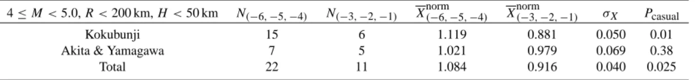
The preliminary results before earthquakes with magni-tude 4.0 ≤ M < 5.0, R < 200 km, H < 50 km are presented in Table 3. The probability that increasing takes place before weak earthquakes is equal to (1 − P ) = 0.97 (Table 3). The available data points are not large enough to make statisti-cally proved conclusion but one could assume that the semi transparency decreasing depends on magnitude and R.
Table 3. The modifications of the averaged normalized coefficient of semi transparency for different stations before earthquakes. The columns, marked as (N(−6, −5, −4)), and (N(−3, −2, −1)) mean the number of earthquakes, for which the semi transparency coefficients in
(−6, −5, −4) nights was greater than in the (−3, −2, −1) nights. In the next two columns marked as (Xnorm(−6, −5, −4)) and (Xnorm(−3, −2, −1)), the normalized coefficients of semi transparency averaged per group of earthquakes are represented. The values were obtained by the superposed epoch method. The next column contains the mean deviations (σX), that were obtained by a random procedure. Last column represents the probability (Pcasual) of the fact that the decreasing of the semi transparency coefficient is casual. The line “total” represents this probability
for all stations together
4 ≤ M < 5.0, R < 200 km, H < 50 km N(−6, −5, −4) N(−3, −2, −1) X(−norm6, −5, −4) Xnorm(−3, −2, −1) σX Pcasual
Kokubunji 15 6 1.119 0.881 0.050 0.01
Akita & Yamagawa 7 5 1.021 0.979 0.069 0.38
Total 22 11 1.084 0.916 0.040 0.025
4 Discussion and conclusions
Now the new results of the present work will be discussed in connection to possible interpretation on the basis of physical mechanisms of lithosphere-ionosphere coupling, that were proposed in literature.
Using vertical sounding stations, it was shown that the semi transparency coefficients of the Es-layers decreased 1– 3 days before and increased 1-3 days after earthquakes with magnitudes M > 5, depths H < 100 km and R < 300 km. We also obtain preliminary results showing that the semi transparency coefficient decreased before earthquakes with magnitudes M > 4 depths H < 50 km and R < 200 km. Only not dense layers were taken into account (frequency
fbEs <2.5 MHz) when we calculate the coefficients of semi transparency.
According to Takefu (1989) and Gorbunova and Shved (1984), the semi transparency coefficient characterizes the existence of small scale inhomogeneities of electron concen-tration in the sporadic layers, or in other words, the level of small scale wave turbulence of the ionospheric plasma. The decreasing of the semi transparency coefficient allows to sup-pose that, 1–3 days before earthquakes, heating takes place in the ionosphere that decreases the level of turbulence due to the increasing of diffusion.
What can be the origin of this heating? Two possible mechanisms of disturbances transmission from the region of earthquake preparation in the crust to ionospheric E-region have been already discussed by Liperovsky et al. (2000), Gokhberg and Shalimov (1996), and Sorokin et al. (1998). The first one is the so called “acoustic” mechanism when it was supposed that, in the region of earthquake preparation, low frequency acoustic noise (f = 0.01÷1 Hz) is generated. Amplitudes of acoustic waves increase when they propagate up to altitudes larger than 100 km and, in sporadic layers, generation of local electrical fields and currents induce heat-ing due to collisions between ions and neutrals (Liperovsky et al., 1997; Haldoupis et al., 1997).
Another mechanism refers to the so called “electrical” one. In this case it is supposed that a few days before earthquakes, local atmospheric electric fields of lithosphere origin arise,
change electric field at altitudes up to 100 km, and gener-ate corresponding local electric currents, caused heating in E-region (Gokhberg et al., 1995; Sorokin et al., 1998; Kim and Hegai, 1985). One could suppose that, under specific conditions, ionospheric effects were caused by one of these mechanisms, and in other conditions they were caused by other mechanism. In both cases, local generation of electric fields and local current systems lead to the heating and to the decrease in the semi transparency coefficient due to sufficient decreasing of foEs (while fbEsdoes not change or changes a little).
Let us compare the results of the present work with the results of Silina et al. (2001). In this paper, a small de-creasing of the semi transparency coefficient was also re-vealed for 20 strong (M ≥ 5.5) and deep H > 33 km earthquakes at distances R < 500 km. However for strong (M ≥ 5.5) earthquakes occurring close to the Earth’s surface (H = 3 ÷ 5 km), on the contrary a significant increasing of the semi transparency coefficient was revealed. This points out at another mechanism of generation of disturbances in the ionosphere. It must be emphasized that in Silina et al. (2001) there were no limitations on fbEs, i.e. coefficients for both dense and not dense layers were used in the analysis. Prob-ably for strong earthquakes close to the Earth’s surface the more intensive generation of inhomogeneities in E-region was caused by drift gradient instability, which has a thresh-old, as it is well known. Only very strong earthquakes close to the surface can generate sufficient spikes of electric fields, and then could trigger this instability.
Acknowledgement. This work was partly supported by RFBR No.
02-05-64493, by the International Space Science Institute (ISSI) at Bern, Switzerland within the project “Earthquakes influence of the ionosphere as evident from satellite plasma-density electric field data” and by the Commission of the EU (grant No. INTAS-01-0456).
References
Gokhberg, M. B., Morgounov, V. A., and Pokhotelov, O. A.: Earth-quake Prediction: Seismoelectromagnetic Phenomena, Reading-Philadelphia, Gordon and Breach Science Publishers, 287, 1995.
284 E. V. Liperovskaya et al.: Variability of sporadic E-layer semi transparency
Gokhberg, M. B., Nekrasov, A. K., and Shalimov, S. L.: On the influence of an unstable emanation of gases in seismically active regions of the ionosphere, Izv, Physics of the Solid Earth, 8, 52– 55, 1996.
Gorbunova, T. A. and Shved, G. M.: The analysis of Es
-semi-transparency as an indicator of turbulence with dynamically ho-mogeneous conditions, Geomagnetism and Aeronomy, 24, N1, 30–34, 1984.
Haldoupis, C., Farley, D. T., and Schlegel, K.: Type-1 echoes from the mid-latitude E-region ionosphere, Ann. Geophysicae, 15, 908–917, 1997.
Kim, V. P. and Hegai, V. V.: Effect of the electric field on the night-time E-region of the middle latitude ionosphere, Geomagnetism and Aeronomy, 25, 5, 855–856, 1985.
Liperovsky, V. A., Pokhotelov, O. A., and Shalimov, S. L., Ionosphere-ionosphere connections before earthquakes, Nauka, Moscow, (in Russian), 304, 1992.
Liperovsky, V. A., Meister, C.-V., Schlegel, K., and Haldoupis, Ch.: Currents and turbulence in and near mid-latitude sporadic E-layers caused by strong acoustic impulses, Ann. Geophysicae, 15, 767–773, 1997.
Liperovsky, V. A., Senchenkov, S. A., Liperovskaya, E. V., Meister, C.-V., Rubtsov, L. N., and Alimov, O. A.: Studying disturbances in temporal variations of the frequency fbEs of the nighttime
mid-latitude Es-layer on the basis of minute measurements,
Ge-omagnetism and Aeronomy, 39, 1, 124–127, 1999.
Liperovsky, V. A., Pokhotelov, O. A., Liperovskaya, E. V., Parrot, M., Meister, C.-V., and Alimov, A.: Modification of sporadic
E-layers caused by seismic activity, Surveys in Geophysics, 21, 449–486, 2000.
Mathews, J. D.: Sporadic E: current views and recent progress, J. Atmospheric and Terrestrial Physics, 60, 4, 413–435, 1998. Ondoh, T. and Hayakawa, M.: Seismo discharge model of
anomalous sporadic E ionization before great earthquakes, in: Seismo Electromagnetics. Lithosphere-Atmosphere-Ionosphere Coupling, (Eds) Hayakawa, M. and Molchanov, O. A., TERRA-PUB, Tokyo, 385–390, 2000.
Parrot, M. and Mogilevsky, M.: VLF emissions associated with earthquakes and observed in the ionosphere and the magneto-sphere, Phys. Earth and Planet. Inter., 57, 86–99, 1998. Silina, A. S., Liperovskaya, E. V., Liperovsky, V. A., and Meister,
C.-V.: Ionospheric phenomena before strong earthquakes, Natu-ral Hazards and Earth System Sciences, 1, 1–6, 2000.
Sorokin, V. M., Chmirev, V. M., Pokhotelov, O. A., and Liperovsky, V. A.: Review of the models of lithospheric-ionospheric links during earthquake preparation process, Proceed. of the Confer-ence: Short-term prognosis a disastrous earthquakes using radio physical ground-based and space methods, (Eds) Strakhov, V. N. and Liperovsky, V. A., Moscow, 64–87, 1998.
Takefu, M.: Effects of scattering on the partial transparency of spo-radic E-layers, 2. Including the Earth’s magnetic field, J. Geo-magn. and Geoelectr., 41, 8, 699–726, 1989.
Whitehead, J. D.: Recent work on mid-latitude and equatorial sporadic-E, J. Atmospheric and Terrestrial Physics, 51, 5, 401– 424, 1989.