The spatial variability of snow water equivalent

(1)

HAL Id: hal-00298841

https://hal.archives-ouvertes.fr/hal-00298841

Submitted on 8 Jun 2007

HAL is a multi-disciplinary open access

archive for the deposit and dissemination of sci-entific research documents, whether they are pub-lished or not. The documents may come from teaching and research institutions in France or abroad, or from public or private research centers.

L’archive ouverte pluridisciplinaire HAL, est destinée au dépôt et à la diffusion de documents scientifiques de niveau recherche, publiés ou non, émanant des établissements d’enseignement et de recherche français ou étrangers, des laboratoires publics ou privés.

The spatial variability of snow water equivalent

T. Skaugen

To cite this version:

T. Skaugen. The spatial variability of snow water equivalent. Hydrology and Earth System Sciences Discussions, European Geosciences Union, 2007, 4 (3), pp.1465-1489. �hal-00298841�

(2)

HESSD

4, 1465–1489, 2007 Spat-var-SWE T. Skaugen Title Page Abstract Introduction Conclusions References Tables Figures ◭ ◮ ◭ ◮ Back Close

Full Screen / Esc

Printer-friendly Version Interactive Discussion

EGU

Hydrol. Earth Syst. Sci. Discuss., 4, 1465–1489, 2007 www.hydrol-earth-syst-sci-discuss.net/4/1465/2007/ © Author(s) 2007. This work is licensed

under a Creative Commons License.

Hydrology and Earth System Sciences Discussions

Papers published in Hydrology and Earth System Sciences Discussions are under open-access review for the journal Hydrology and Earth System Sciences

The spatial variability of snow water

equivalent

T. Skaugen

Norwegian Water Resources and Energy Directorate, P.O. Box 5091, Maj, 0301, Oslo, Norway Department of Geosciences, University of Oslo, P.O. Box 1047, Blindern, Oslo, Norway Received: 16 May 2007 – Accepted: 23 May 2007 – Published: 8 June 2007

Correspondence to: T. Skaugen (ths@nve.no)

(3)

HESSD

Full Screen / Esc

EGU Abstract

The spatial distribution of snow water equivalent (SWE) is modelled as a two parameter gamma distribution. The parameters of the distribution are dynamical in that they are functions of the number of accumulation and ablation events and the temporal correla-tion of accumulacorrela-tion and ablacorrela-tion events. The estimated spatial variability is compared 5

to snow course observations from the alpine catchments Norefjell and Aursunden in Southern Norway. A fixed snow course at Norefjell was measured 26 times during the snow season, which showed that the spatial coefficient of variation change during the snow season with a decreasing trend from the start of the accumulation period and a sharp increase in the ablation period. The gamma distribution with dynamical param-10

eters reproduced the observed spatial statistical features of SWE well both at Norefjell and Aursunden. Also the shape of simulated spatial distribution of SWE agreed well with the observed at Norefjell. The temporal correlation tends to be positive for both accumulation and ablation events. However, at the start of ablation, a better fit be-tween modelled and observed spatial standard deviation of SWE is obtained by using 15

negative correlation between SWE and melt.

1 Introduction

A major cause of severe flooding in Norway is the combination of intense snowmelt and heavy precipitation. In order to forecast these events, we need reliable forecasts of precipitation and temperature and a good estimate of the snow reservoir and its 20

coverage in the catchment at the time of the forecast. The dynamics of runoff due to snowmelt, and thus the water balance in the melting season, is very dependent on the evolution of snow free areas, which again is closely linked to the spatial distribution of snow water equivalent (SWE) (Pomeroy et al., 2004; Luce et al., 1998; Buttle and McDonnel, 1987). The shape of the distribution is important in order to describe the 25

development of snow free areas in spring. A skewed distribution with high frequencies 1466

(4)

HESSD

Full Screen / Esc

EGU

of small values of SWE would produce more snow free areas in response to uniformly distributed melt than would a more normal distribution of SWE where the highest fre-quencies are found for higher values of SWE. Increased production of snow free areas for skewed distributions will occur in cases where the spatial distribution of daily melt is inversely correlated to the distribution of SWE as reported by Faria et al. (2000). 5

Positively skewed distributions like the exponential (Gao and Sorooshian, 1994) and gamma (Onof et al., 1998; Mackay et al., 2001) have often been favoured for describ-ing the spatial distribution of daily precipitation. As the accumulated SWE is the sum of such positively skewed and correlated variables, one would expect the distribution of SWE to be subject to the central limit theorem (Feller, 1971, p. 258) and being less 10

skewed than the distribution of the individual snowfall events. The normal distribution has often been found to be a good model for describing SWE at its seasonal maximum (Marchand and Killingtveit, 1999, 2002; Alfnes et al., 2004), which indicates that the spatial distribution of SWE evolves from a rather skewed distribution at the beginning of the snow season towards a less skewed, (even normal) distribution at its seasonal 15

maximum. The Swedish HBV model (Bergstrøm, 1992; Sælthun, 1996) is used opera-tionally for flood forecasting at the Norwegian Water Resources and Energy Directorate (NVE) and has been supplemented with a snow routine developed for use in Norway which accounts for the development of the snow reservoir and the snow coverage at different altitude levels (Killingtveit and Sælthun, 1995). This routine is developed un-20

der the assumptions that precipitation as snow is log-normally distributed in space with a fixed coefficient of variation. Donald et al. (1995) presented a snow accumulation model where, once the snow coverage was 100%, the spatial variability of SWE re-mained constant. These static ways of representing the spatial distribution of SWE are thus in conflict with the central limit theorem, reported observations (Alfnes et al., 2004; 25

Pomeroy et al., 2004) and observations presented in this paper.

Skaugen et al. (2004) put forward a formulation for the spatial distribution of snow, using the fact that when individual snowfall events are gamma distributed, the distribu-tion of accumulated snowfall events is also gamma distributed with parameters derived

(5)

HESSD

Full Screen / Esc

EGU

from the parameterisation of individual snowfall events and the number of accumula-tions. This model is constrained by assumptions of independence in time, but takes into account that the statistical features of the spatial distribution of snow water equivalent (SWE) change during the season, as demonstrated observations. The dynamical as-pect of the shape of the spatial distribution of SWE is a feature that has to be included 5

in the modelling of SWE in order to simulate realistic snow distributions

Observed differences for spatial distributions of SWE at the peak of accumulations has been addressed to landscape and meteorological features such as vegetation type, topography and wind (Erickson et al., 2005; Bruland et al., 2004; Alfnes et al., 2004; Marchand and Killingtveit, 2004; Erxleben et al., 2002; Shook and Gray, 1997). Ac-10

cording to Liston (2004), three mechanisms effective on different spatial scales influ-ence the snowdepth. Snow-canopy interactions in forested regions are important at one to hundreds of meters, snow redistribution by wind on tens to hundreds of metres and orographic influences of precipitation being active on one to a few kilometres. The latter spatial scale is the relevant scale for describing the spatial distribution of SWE in 15

lumped hydrological models such as the operational HBV model. It is the objective of this study to demonstrate that the spatial distribution of SWE can be adequately mod-elled as the summation of correlated (in time) daily precipitation (snowfall) fields. The sources of variability at smaller scales, like snow-canopy interactions and wind drift are, in this study, not taken into account.

20

We want to develop dynamical expressions for the spatial variability of SWE both for the accumulation and ablation season. We further want to use this information to assign analytical expressions for the spatial distribution of SWE. The proposed method-ology will be validated against time series of the spatial distribution of SWE measured at locations in the mountains in Southern-Norway.

25

The next section presents the derivation of expressions for the spatial moments of SWE, where temporal correlation is taken into account. The moments are then used for estimating the parameters of the spatial distribution of SWE. The following sec-tion presents a snow monitoring campaign specially designed for studying the spatial

(6)

HESSD

Full Screen / Esc

EGU

distribution of SWE throughout the snow season. In the fourth section the modelled moments and distributions are tested against observed data and discussed, whereas conclusions are found in the final section.

2 Modelling the accumulation and ablation of snow as sums of correlated

gamma distributed variables

5

When modelling the spatial distribution of SWE, we have to take into account the history of accumulation and ablation events up to the time of interest. In Skaugen et al. (2004) this was carried out by modelling the spatial distribution of SWE as sums of identical independently distributed variables of the two parameter gamma distribution. Here, the spatial distribution of SWE is also modelled within the framework of the two parameter 10

gamma distribution, but, through a simple procedure, the effect of temporal correlation is introduced.

Let us assume that every snow fall event can be described as a collection of gamma distributed unit snowfalls y. The unit snowfall y is distributed in space according

to a two-parameter gamma distribution, y=G(ν0, α₀), with probability density function 15 (PDF): fα₀,ν₀(y) = 1 Γ(ν0) αν0 0 y ν0−1_e−α0y _α 0, ν0, y > 0 (1)

where α₀ and ν₀ are parameters. The mean equals E (y)=ν0/α₀ and the variance equals Var(_y)=ν0/α2₀. The choice of distribution is motivated partly from studies report-ing the gamma distribution as a suitable choice of spatial distribution for precipitation 20

(Onof et al., 1998; Mackay et al., 2001) and SWE (Kutchment and Gelfan, 1996) and partly because of the practical mathematical features of the gamma distribution and the flexibility needed for representing the observed changes in the shape of the spatial distribution during the snow season. We want to describe the moments of the

(7)

HESSD

Full Screen / Esc

EGU

lated snow reservoir_{z(t), accumulated at time t, z(t)=}

n(t)_P

i =1

yi, wheren is the number of unitsy accumulated up to the time t. The mean of z(t)is

E (z(t)) = n X i =1 E (yi) = n ν₀ α₀, (2)

whereas for the variance ofz(t) we have to take into account the temporal correlation

ofy and we have to consider the covariance matrix of z(t) (see Haan, 1977, p. 56):

5 Var(_{z(t)) =} n(t) X i =1 Var(yi) + 2 X i <j Cov(yi, yj) (3)

In the following, we assume that the covariance between the units can be de-scribed as a constant fraction c of the variance, Var(y), of the individual y’s,

Cov(yi, yj)=cVar(y)=c

ν₀

α2

0

. The variance ofz(t) becomes:

Var(_{z(t)) = n}ν0 α2₀ + n(n − 1)c ν₀ α₀2 = n ν₀ α2₀(1 + (n − 1)c) (4) 10

We note thatc=Cov(yi,yj)

Var(y) is the correlation coefficient, given that yi andyj are identically distributed and represents the average temporal correlation for all then units.

We want the spatial distribution of accumulated snowz(t) at all times to be simple

mathematically tractable distribution function, with which we easily can simulate and perform other exploratory analyses. We thus state thatz(t) is distributed as a gamma

15

distribution with parametersnν_n and α_n. This implies that the n elements of the sum

are independent, and identically gamma distributed variables with parametersνn and

αn (see Feller, 1971, p. 47). Let us denote these independent variables as Yi. The mean and variance ofz(t) modelled as a sum of independent variables, Y are:

E (z(t)) = n_ανn

n

(5) 20

(8)

HESSD

Full Screen / Esc

Printer-friendly Version Interactive Discussion EGU and Var(z(t)) = nνn α2_n (6)

From the mean and variance ofz(t) modelled as a sum of dependent variables, y, we

can determine expressions forν_nandα_nby the mean and variance ofz(t) modelled as

a sum of independent variables,Y . From the equating Eqs. (2) and (5), nν0

α0=n νn αn and 5 Eqs. (4) and (6),nν0 α₀2(1+(n−1)c)=n νn

α_n2 we can solve forνnandαnand get:

αn= α₀ 1 + (n − 1)c (7) and ν_n= ν0 1 + (n − 1)c (8)

We note that the ratios νn

αn and

ν₀

α0 are equal, which mean that the mean of the process 10

is unaffected by the correlation.

2.1 Adding correlated variables to a sum of independent variables

Let us say at timet′ _{an additional snowfall of}_{u units of y, have fallen on z(t) giving us}

the snow reservoirz(t′_), z(t′_{) = Y}

1+ Y2+ .. + Yn+ y1+ y2+ .. + yu (9)

15

The mean can be estimated straightforwardly as the sum of the individual means:

E (z(t′_{)) =} n X i =1 E (Yi) + u X i =1 E (yi) = n ν_n α_n + u ν₀ α₀ (10)

For the variance of z(t′_{) we must again consider the covariance matrix of Var(}_z(t′₎₎

and V ar(z(t′_{)) is the sum of all the elements of the covariance matrix. In Fig. 1 we}

(9)

HESSD

Full Screen / Esc

EGU

see an example of_{n=3 and u=2. Given that the Y ’s are uncorrelated, the covariance} elements describing the covariance between theY ’s are zero and we get the following

expression for the variancez(t′_):

Var(z(t′₎₎₌ n X j =1 Var(Yj)+2 n X j=1 u X i =1 Cov(Yj, yi)+ u X i =1 Var(yi)+2 u−1 X i =1 u X k=i+1 Cov(yi, yk) (11)

We assume also here that Cov(_{Y, y) can be approximated by Cov(Y, y)=cVar(y)=c}ν0

α2

0 , 5

and Eq. (11) can be written as: Var(z(t′_{)) = n}νn α_n2 + u ν0 α2₀ + 2nuc ν0 α2₀ + u(u − 1)c ν0 α2₀ (12)

From Eqs. (10) and (12), we can develop expressions for the parameters of the distri-butions ofz(t′_{) modelled as a sum of}_{n + u independent gamma distributed events with}

momentsE (z(t′

))=nνn+u

α_n+u and Var(z(t

′ ))=nνn+u α2 n+u : 10 α_n+u= (_{n + u)}νn αn nνn α2 n + ν0 α2 0 (_{u + 2nuc + u(u − 1)c)} (13) and ν_n+u= (_{n + u)(}νn αn) 2 nνn α2 n + ν₀ α2 0 (_{u + 2nuc + u(u − 1)c)} (14) 2.2 Melting events

We can, in a similar way as above, develop the moments for the accumulated SWE 15

after a melting event. Let us say at timet′_{a melting event takes place and}_{u units of y,}

are melted fromz(t) giving us the snow reservoir z(t′_), z(t′_{) = Y}

1+ Y2+ .. + Yn− y1− y2− .. − yu (15)

(10)

HESSD

Full Screen / Esc

EGU

We make here the assumption that the spatial distribution of a unit melt is identical to that of a unit snowfall. It is difficult to have strong assumptions on the spatial distribu-tion of snow melt, other than that the ultimate melting event is necessarily identically distributed as the ultimate SWE. Essery and Pomeroy (2004) assumed a log-normal distribution of snowmelt from log-normally distributed SWE, a distribution of melt which 5

is similar in shape to the gamma distribution. The mean can, as above, be estimated straightforwardly as the sum of the individual means:

E (z(t′_{)) =} n X i =1 E (Yi) − u X i =1 E (yi) =n ν_n α_n − u ν₀ α₀ (16)

Figure 2 shows the covariance matrix of Var(z(t′_{))and we have the following expression}

for the variance ofz(t′_):

10 Var(z(t′_{)) =} n X j=1 Var(Y_j) − 2 n X j=1 u X i =1 Cov(Y_j, y_i)+ u X i =1 Var(y_i) + 2 u−1 X i=1 u X k=i+1 Cov(y_i, y_k) (17)

We get negative and positive covariance contributions from the melting event. The neg-ative contributions come from when the melting event is correlated to the snow reser-voir prior to the melting. A melting unit correlated with a melting unit gives a positive contribution. Also here we make the assumption that Cov(Y, y)can be approximated by

15

Cov(_{Y, y)=cVar(y)=c}ν0

α₀2, and Eq. (17) can be written as: Var(z(t′_{)) = n} ν α2 + u ν₀ α2₀ − 2nuc ν₀ α2₀ + u(u − 1)c ν₀ α2₀ (18)

From Eqs. (16) and (18), we can develop expressions for the parameters of the distri-butions ofz(t′_{) modelled as}_{n−u independent gamma distributed events:}

α_n−u= (n − u)νn α_n nνn α2n + ν₀ α2₀(u − 2nuc + u(u − 1)c) (19) 20 1473

(11)

HESSD

Full Screen / Esc

Printer-friendly Version Interactive Discussion EGU and ν_n−u= (_{n − u)(}νn αn) 2 nνn α2_n + ν0 α₀2(u − 2nuc + u(u − 1)c) (20)

3 Snow course data from Norefjell – Southern Norway

During the EU project Envisnow, montoring of the spatial distribution of SWE during the snow season was performed at Norefjell (60◦₁₅′_{N, 9}◦₃₀′_{E) located in southern Norway}

5

110 km north-east of Oslo (see Fig. 3). The motivation for the monitoring campaign was to study the possible change in features of the spatial distribution of SWE trough the snow season. The snow monitoring campaign was carried out doing snow surveys every second week in the accumulation season and every week during the melting season. The route was fixed (by GPS) for the 2 km long snow course and snow depth 10

was measured every 10 m. Snow density was measured twice during the snow course at locations of the mean snow depth. The snow course route is located at 1100 m a.s.l. and is above the tree line. 17 one-day campaigns between November 2002 and June 2003, and 9 campaigns between October 2003 and February 2004 were carried out. The latter part of the monitoring period also includes the start of the accumulation 15

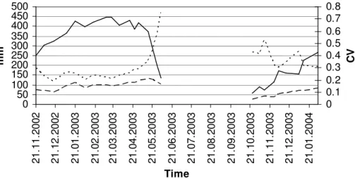
period, whereas the former started when there were already 200 mm of SWE present. Figure 4 shows the time series of the mean, standard deviation and coefficient of variation (CV) of SWE for the snow course data. We can note that the CV (see Octo-ber 2003) is relatively high at the start of the accumulation season, decreases during the accumulation season, and rises sharply during the melting season. As the mean 20

SWE and the standard deviation both decrease during the melting season, the increas-ing CV implies that the rate of change (decrease) of the mean is much higher than for the standard deviation. This feature of the spatial standard deviation of SWE was also noted by Pomeroy et al. (2004), who found that the otherwise strong association

(12)

HESSD

Full Screen / Esc

EGU

tween mean SWE and standard deviation was not evident during melt. During melt, the mean SWE declined whereas the standard deviation increased or remained constant.

4 Results and discussion

The dynamical parametersα and ν of the two parameter gamma distribution was

cal-culated for each point of observation of SWE, taking into account accumulation and 5

ablation events by using the Eqs. (13) and (14), or (19) and (20), respectively. The ini-tial parametersα0andν0were estimated from the daily mean (m=5.86 mm) and

stan-dard deviation (_{s=7.57 mm) of precipitation data (zero values was excluded) trough the} relationsα₀=m/s2 andν₀=m2/s2. The precipitation station is located 18 km south of the snow course site and at 367 m a.s.l. The correlation coefficient c was tuned in 10

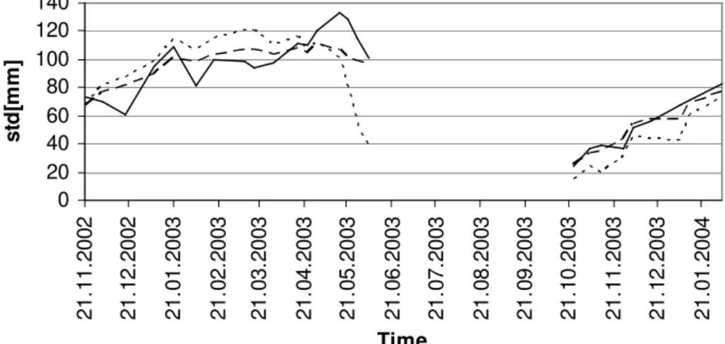
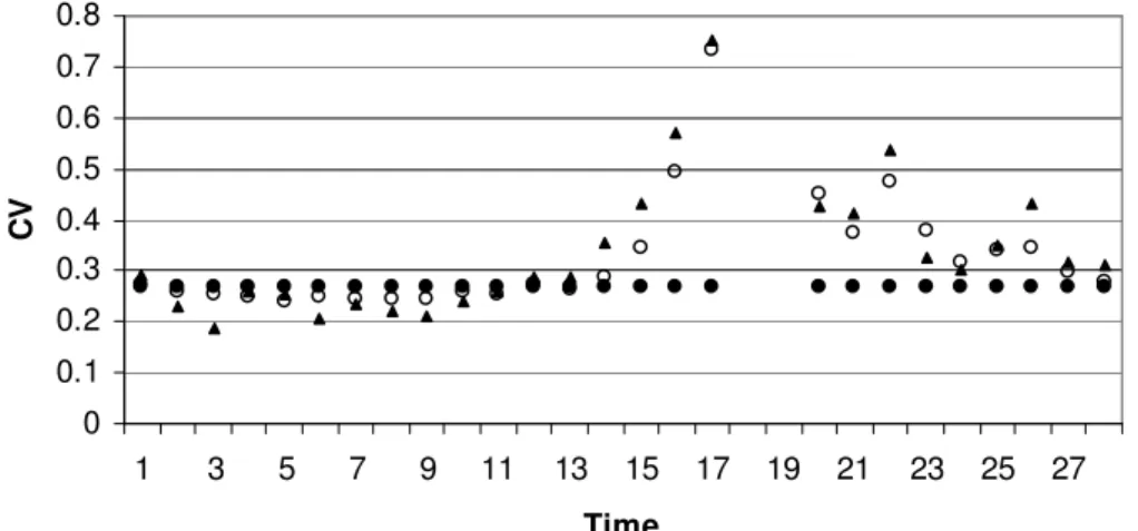
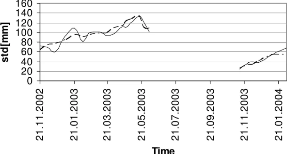
order to get an optimal fit as measured by the Nash and Sutcliffe coefficient of effi-ciency R2 (Nash and Sutcliffe, 1970). The estimated time series of standard deviation and CV of SWE is also compared to that estimated by the traditional snow routine of the HBV models which uses a lognormal distribution with a fixed CV (optimized by the R2 criterion). Figure 5 shows observed and estimated (by the proposed model and 15

by HBV) values of the spatial standard deviation of SWE and Fig. 6 shows observed and estimated CV. The R2 value for the estimate of the spatial standard deviation was R2=0.86 for the new model, and R2=0.32 for the snow routine of the HBV model. The new model is thus a considerable improvement to the lognormal distribution with a fixed CV. The observed values do indeed show that the spatial distribution of SWE changes 20

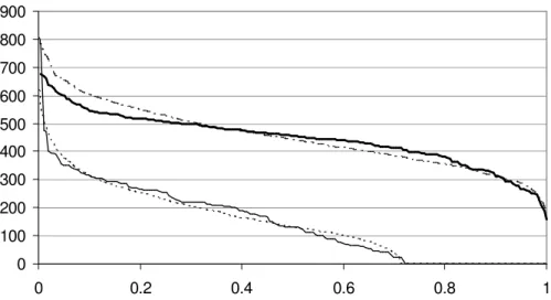
through the season, and the proposed model capture these changes well. Figure 7 shows the agreement between the gamma CDFs (1000 values are simulated) based on the estimated values ofα and ν and the empirical CDFs from the observations for

the dates 18 March 2003 and 28 May 2003, confirming that a representative model for the spatial distribution of SWE is developed.

25

The values forα0andν0were estimated from the mean and the standard deviation

of days with precipitation from the time series of a single precipitation station. Asα₀

(13)

HESSD

Full Screen / Esc

EGU

and ν₀ is assumed to represent the parameters of the spatial distribution of a unit of snowfall, estimating the values from a single time series implies an ergodic precipi-tation process where the spatial and the temporal distribution is equal. Whereas no rigorous study of ergodicity for this area was undertaken, it is interesting to note that the estimated values we obtained forα₀andν₀gave good results. The values ofα₀and 5

ν₀were varied while keeping a constant mean (_{E (y)=}ν0

α₀=const) and no improvements in the estimation of the spatial standard deviation of SWE were observed.

The optimal values for_{c in the Norefjell data was c=0.019. Using different values} of c for accumulation and ablation events were tried and, for this location,

improve-ments of R2 were found. When usingc=0.01 on ablation events, we obtained R2=0.9.

10

Studies of temporal correlation of precipitation, both for a fixed coordinate system and from a coordinate system that moves with the storm, show a rapidly declining correla-tion funccorrela-tion which approaches zero after approximately two hours (Zawadski, 1973). As the parameter c represents a temporal average over the total number of events,

it is thus not strange that the values obtained in this study are small. The effect of 15

correlation, however, is significant, in that we would otherwise have a steadily increas-ing spatial variance as both summation and subtraction increases the variance (Haan, 1977). It is interesting to note that also the correlation between ablation events and SWE prior to melting turns out to be positive. Similar findings are reported by Pomeroy et al. (2004) who found positive correlation on the catchment scale (>10 km2). For the 20

particular study of Pomeroy et al. (2004), negative correlations between pre-melt SWE and melt where found for scales smaller than the catchment scale. Positive correlation is explained by the presence of landscape classes (shrub tundra) receiving more snow due to redistribution processes and the possibility of increased melt rate for areas with exposed shrub due to reduced albedo and enhanced aerodynamic roughness. We 25

investigated the effects of varying the sign of the correlation coefficient c in Eq. (17) for ablation and for different phases of the ablation process. A negative correlation between melt and pre-melt SWE resulted in a steadily increasing standard deviation during the melting period and was thus not consistent with the observations. Negative

(14)

HESSD

Full Screen / Esc

EGU

correlation at the beginning of the melting period and positive towards the end im-proved the fit between modelled and observed standard deviation of SWE (R2=0.92) (see Fig. 8) and we note that the increase in standard deviation seen at the start of the melting season (see Fig. 8 when the mean SWE starts to decrease) is now well estimated due to negative correlation. A possible reason for an initial negative correla-5

tion can be the smaller demand of energy needed by shallow snow packs to reach an isothermal state and the maximum amount of retainable melt water in the snow pack. Melting will thus take place earlier for these shallow snow packs. The positive correla-tion is harder to explain if one does not take into account dominating landscape classes that favour both accumulation and increased melt rate. Such landscape classes are not 10

present at the Norefjell snow course, where there are some 30–40 m of low-growing willow thicket (<60 cm) and otherwise no vegetation besides grass. Maybe the positive

correlation becomes appropriate only towards the end of the ablation season, when the entire snow pack is mature and producing melt. At this stage, SWE starts to be a lim-iting factor and more melt water is generated from larger snow packs simply because 15

more SWE is available for melting.

In order to investigate whether the method could be applied also to other locations than Norefjell we tested if the spatial variability of SWE could be reproduce at an alpine catchments at Aursunden in the northern part of Southern Norway (see Fig. 1). Snow course measurements was carried out at Aursunden (930 m a.s.l.) three times during 20

April and May in 2002 (see Alfnes et al., 2004). Again, the route was fixed by GPS for the 1 km long snow course and snow depth was measured every 10 meters. The pa-rametersα0andν0were estimated in the same manner as above from the daily mean, m=3.31 mm, and daily standard deviation, s=4.08 mm, (zero events excluded) of

pre-cipitation measured at a prepre-cipitation station (685 m a.s.l.) located 10 km southeast 25

of the snow course. The correlation coefficient was tuned to the values of observed spatial standard deviation. Also here the best fit was obtained with using different val-ues ofc for ablation (c=0.12) and accumulation (c=0.14) events. Figure 9 shows the

good agreement between observed and modelled spatial standard deviation and CV. 1477

(15)

HESSD

Full Screen / Esc

EGU

The correlation coefficient and the temporal standard deviation of precipitation take on quite different values at Norefjell and Aursunden. Although the observations points are too few to make strong inferences it does seem reasonable that we find low temporal correlation with relatively high temporal variability of precipitation. The same effect of high spatial variability and short spatial correlation lengths is observed in the spatial 5

domain for precipitation (Skaugen, 1997).

5 Conclusions

A model for the spatial distribution of SWE has been put forward. At all times the spatial distribution of SWE can be expressed as a two parameter gamma distribution where the parameters are functions of the mean and variability of observed precipitation, the 10

number of accumulation and ablation events and of temporal correlation.

The observed time series of SWE confirms that the spatial distribution of SWE do change trough the snow season with initially high CV, which decreases during the accumulation season and increases in the melting season. These features, as well as the shape of spatial distributions of SWE, are well reproduced by the proposed model. 15

The new model clearly represents the spatial distribution of SWE more realistically than the log-normal distribution with a fixed CV which is traditionally used in the HBV model in the Nordic countries. The model provides good estimates of the spatial vari-ability of SWE at two alpine locations in Southern Norway.

Analysis of the correlations between pre melt SWE and melt suggests that correlation 20

is negative in the early stages of the ablation process and positive at later stages. Positive correlation between SWE and melt at the end of the ablation proved, within the model framework, to be necessary in order to model the decrease in spatial variability observed in the snow course data.

Acknowledgements. The efforts of my colleagues E. Alfnes, L. Andersen, H. C. Udnæs, 25

L. E. Petterson and S. Beldring for collecting the validation data are gratefully acknowledged.

(16)

HESSD

Full Screen / Esc

EGU References

Alfnes, E., Andreassen, L. M., Engeset, R. V., Skaugen, T., and Udnæs, H.-C.: Temporal variability in snow distribution, Ann. Glaciol., 38, 101–105, 2004.

Bergstr ¨om, S.: The HBV model – its structure and applications, SMHI Hydrology, RH no.4, Norrk ¨oping, 35 pp., 1992.

5

Bruland, O., Liston, G. E., Vonk, J., Sand, K., and Killingtveit, ˚A.: Modelling the snow distribution at two high artic sites at Svalbard, Norway, and at an alpine site in central Norway, Nord. Hydrol., 35(3), 191–208, 2004.

Buttle, J. M. and McDonnel, J. J.: Modelling the areal depletion of snowcover in a forested catchment, J. Hydrol., 90, 43–60, 1987.

10

Donald, J. R., Soulis, E. D., Kouwen, N., and Pietroniro, A.: A land cover-based snow cover rep-resentation for distributed hydrologic models, Water Resour. Res., 31(4), 995–1009, 1995. Erickson, T. A., Williams, M. W., and Winstral, A.: Persistence of topographic controls on the

spatial distribution of snow in rugged mountain terrain, Colorado, United States, Water Re-sour. Res., 41, W04014, doi:10.1029/2003WR002973, 2005.

15

Essery, R. and Pomeroy, J.: Implications of spatial distributions of snow mass and melt rate for snow-cover depletion: theoretical considerations, Ann. Glaciol., 38, 261–265, 2004.

Erxleben, J., Elder, K., and Davis, R.: Comparison of spatial interpolation methods for estimat-ing snow distribution in the Colorado Rocky Mountains, Hydrol. Processes, 16, 3627–3649, 2002.

20

Faria, D. A., Pomeroy, J., and Essery, R.: Effect of covariance between ablation and snow water equivalent on depletion of snow-covered in a forest, Hydrol. Earth Syst. Sci., 14, 2683–2695, 2000,http://www.hydrol-earth-syst-sci.net/14/2683/2000/.

Feller, W.: An introduction to probability theory and its applications, John Wiley, New York, pp. 669, 1971.

25

Gao, X. and Sorooshian, S.: A stochastic precipitation disaggregation scheme for GCM appli-cations, J. Climate, 7(2), 238–247, 1994.

Haan, C. T.: Statistical methods in hydrology, The Iowa State University Press, Ames, Iowa, 378 pp., 1977.

Killingtveit, ˚A. and Sælthun, N.-R.: Hydrology, vol. 7 in Hydropower development, NIT,

Trond-30

heim, Norway, 1995.

Kutchment, L. S. and Gelfan, A. N.: The determination of the snowmelt rate and the meltwater

(17)

HESSD

Full Screen / Esc

EGU outflow from a snowpack for modelling river runoff generation, J. Hydrol., 179, 23–36, 1996.

Liston, G. E.: Representing subgrid snow cover heterogeneities in regional and global models, J. Climate, 17, 1381–1397, 2004.

Luce, C. H., Tarboton, D. G., and Cooley, K. R.: The influence of the spatial distribution of snow on basin-averaged snowmelt, Hydrol. Processes, 12, 1671–1683, 1998.

5

Mackay, N. G., Chandler, R. E., Onof, C., and Wheater, H. S.: Disaggregation of spatial rainfall fields for hydrological modelling, Hydrol. Earth Syst. Sci., 5, 165–173, 2001,

http://www.hydrol-earth-syst-sci.net/5/165/2001/.

Marchand, W.-D. and Killingtveit, ˚A.: Statistical probability distribution of snow on sub-grid cell level, Nordic Hydrological Programme, NHP Report No. 47, pp 461–471, 2002.

10

Marchand, W.-D. and Killingtveit, ˚A.: Statistical properties of snow cover in mountainous catch-ments in Norway, Northern Research Basins, Twelfth International symposium and Work-shop, Reykjavik, Iceland, pp. 227–239, 1999.

Marchand, W.-D. and Killingtveit, ˚A.: Statistical properties of spatial snow cover in mountainous catchments in Norway, Nord. Hydrol., 35(2), 101–117, 2004.

15

Nash, J. E. and Sutcliffe, J. V.: River flow forecasting through conceptual models: Part I – A discussion of principles, J. Hydrol., 10, 282–290, 1970.

Onof, C., Mackay, N. G., Oh, L., and Weather, H. S.: An improved rainfall disaggregation technique for GCMs, J. Geophys. Res., 103(D16), 19 577–19 586, 1998.

Pomeroy, J., Essery, R., and Toth, B.: Implications of spatial distributions of snow mass and

20

melt rate for snow-cover depletion: observations in a subarctic mountain catchment, Ann. Glaciol., 38, 195–201, 2004.

Shook, K. and Gray, D. M.: Synthesizing shallow seasonal snow covers, Water Resour. Res., 33(3), 419–426, 1997.

Skaugen, T.: Classification of rainfall into small and large scale events by statistical pattern

25

recognition, J. Hydrol., 200, 40–57, 1997.

Skaugen, T., Alfnes, E., Langsholt, E., and Udnæs, H.-C.: Time variant snow distribution for use in hydrological models. Ann. Glaciol., 38, 180–186, 2004.

Sælthun, N. R.: The “Nordic” HBV model. Description and documentation of the model version developed for the project Climate Change and Energy Production, NVE Publication no.

7-30

1996, Oslo, 26 pp., 1996.

Zawadzki, I. I.: Statistical properties of precipitation patterns, J. Appl. Meteorol., 12(3), 459– 472, 1973.

(18)

HESSD

Full Screen / Esc

Printer-friendly Version Interactive Discussion EGU ) , (Y₁Y₁

Cov

0

Cov(Y₁,y₁) Cov(Y₁,y₂)

0

Cov(Y2,Y2)

0

Cov(Y2,y1) Cov(Y2,y2)

0

Cov(Y₃,Y₃) Cov(Y₃,y₁) Cov(Y₃,y₂)

) , (y₁ Y₁

Cov Cov(y₁,Y₂) Cov(y₁,Y₃) Cov(y₁,y₁) Cov(y₁,y₂)

) , (y₂ Y₁

Cov Cov(y₂,Y₂) Cov(y₂,Y₃) Cov(y₂,y₁) Cov(y₂,y₂)

Fig. 1. Correlation matrix of the sum of uncorrelated and correlated variables. TheY s are

uncorrelated and theys are correlated.

(19)

HESSD

Full Screen / Esc

Printer-friendly Version Interactive Discussion EGU ) , (Y₁Y₁

Cov 0 0 ₋Cov(Y₁,y₁) ₋Cov(Y₁,y₂)

0 Cov(Y₂,Y₂) 0 −Cov(Y₂,y₁) −Cov(Y2,y2)

0 0 Cov(Y₃,Y₃) −Cov(Y₃,y₁) −Cov (Y3,y2)

) , (y₁Y₁ Cov

− −Cov(y1,Y2) −Cov(y1,Y3) Cov(y1,y1) Cov(y1,y2)

) , (y2 Y1 Cov

− −Cov(y2,Y2) −Cov(y2,Y3) Cov(y2,y1) Cov(y2,y2)

Fig. 2. Correlation matrix of the sum and difference of uncorrelated and correlated variables. TheY s are uncorrelated and the ys are correlated.

(20)

HESSD

Full Screen / Esc

Printer-friendly Version Interactive Discussion EGU 60˚ 64˚ 4 8 12

Oslo

.

Norefjell

Printer-friendly Version Interactive Discussion EGU 0 50 100 150 200 250 w15 w18 w21 Time m m 0 0.1 0.2 0.3 0.4 0.5 0.6 0.7 0.8

Fig. 9. Observed and estimated values of standard deviation and CV at Aursunden for the weeks 15, 18, 21 in 2002. Observed values of standard deviation and CV are represented by solid line and black triangles. Estimated values of standard deviation and CV are represented by long dashed line and open circles.