HAL Id: hal-00867226
https://hal.archives-ouvertes.fr/hal-00867226
Submitted on 13 Feb 2021
HAL is a multi-disciplinary open access archive for the deposit and dissemination of sci-entific research documents, whether they are pub-lished or not. The documents may come from teaching and research institutions in France or abroad, or from public or private research centers.
L’archive ouverte pluridisciplinaire HAL, est destinée au dépôt et à la diffusion de documents scientifiques de niveau recherche, publiés ou non, émanant des établissements d’enseignement et de recherche français ou étrangers, des laboratoires publics ou privés.
Improved calibration of SOIR/Venus Express spectra
Ann Carine Vandaele, Arnaud Mahieux, Séverine Robert, Sophie
Berkenbosch, Roland Clairquin, Rachel Drummond, Vincent Letocart, Eddy
Neefs, Bojan Ristic, Valérie Wilquet, et al.
To cite this version:
Ann Carine Vandaele, Arnaud Mahieux, Séverine Robert, Sophie Berkenbosch, Roland Clairquin, et al.. Improved calibration of SOIR/Venus Express spectra. Optics Express, Optical Society of America - OSA Publishing, 2013, 21 (18), pp.21148-21161. �10.1364/OE.21.021148�. �hal-00867226�
Improved calibration of SOIR/Venus Express
spectra
Ann Carine Vandaele,1,* Arnaud Mahieux,1 Séverine Robert,1 Sophie Berkenbosch,1
Roland Clairquin,1 Rachel Drummond,1 Vincent Letocart,1 Eddy Neefs,1 Bojan Ristic,1
Valérie Wilquet,1 Frédéric Colomer,2 Denis Belyaev,3 and Jean-Loup Bertaux4 1Planetary Aeronomy, Belgian Institute for Space Aeronomy, 3 av. Circulaire, 1180 Brussels, Belgium 2Ecole Polytechnique, Université Libre de Bruxelles, CP165/52, av. F.D. Roosevelt 50, 1050 Brussels, Belgium
3Space Research Institute, 84/32 Profsoyuznaya Str., 117997, Moscow, Russia
4Laboratoire Atmosphères, Milieux, Observations Spatiales, 11 Bd d'Alembert, 78280 Guyancourt, France *[email protected]
Abstract: The SOIR instrument on board the ESA Venus Express mission
has been operational since the insertion of the satellite around Venus in April 2006. Since then, it has delivered high quality IR solar occultation spectra of the atmosphere of Venus. The different steps from raw spectra to archived data are described and explained in detail here. These consist of corrections for the dark current and for the non-linearity of the detector; removing bad pixels, as well as deriving noise. The spectral calibration procedure is described, along with all ancillary data necessary for the understanding and interpretation of the SOIR data. These include the full characterization of the AOTF filter, one of the major elements of the instrument. All these data can be found in the ESA PSA archive.
©2013 Optical Society of America
OCIS codes: (120.6085) Space instrumentation; (120.6200) Spectrometers and spectroscopic instrumentation; (300.6340) Spectroscopy, infrared; (010.0280) Remote sensing and sensors.
References and links
1. D. Nevejans, E. Neefs, E. Van Ransbeeck, S. Berkenbosch, R. Clairquin, L. De Vos, W. Moelans, S. Glorieux, A. Baeke, O. Korablev, I. Vinogradov, Y. Kalinnikov, B. Bach, J. P. Dubois, and E. Villard, “Compact high-resolution space-borne echelle grating spectrometer with AOTF based on order sorting for the infrared domain from 2.2 to 4.3 μm,” Appl. Opt. 45, 5191–5206 (2006).
2. A. Fedorova, O. Korablev, A. C. Vandaele, J. L. Bertaux, D. Belyaev, A. Mahieux, E. Neefs, V. Wilquet, R. Drummond, F. Montmessin, and E. Villard, “HDO and H2O vertical distributions and isotopic ratio in the Venus
mesosphere by Solar Occultation at Infrared spectrometer onboard Venus Express,” J. Geophys. Res. 113, E00B22 (2008), doi:10.1029/2008JE003146.
3. A. Mahieux, A. C. Vandaele, S. Robert, V. Wilquet, R. Drummond, F. Montmessin, and J. L. Bertaux, “Densities and temperatures in the Venus mesosphere and lower thermosphere retrieved from SOIR on board Venus Express: Carbon dioxide measurements at the Venus terminator,” J. Geophys. Res. 117(E7), E07001 (2012), doi:10.1029/2012JE004058.
4. A. Mahieux, A. C. Vandaele, R. Drummond, S. Robert, V. Wilquet, A. Fedorova, and J. L. Bertaux, “Densities and temperatures in the Venus mesosphere and lower thermosphere retrieved from SOIR onboard Venus Express: Retrieval technique,” J. Geophys. Res. 115(E12), E12014 (2010), doi:10.1029/2010JE003589. 5. A. C. Vandaele, M. De Mazière, R. Drummond, A. Mahieux, E. Neefs, V. Wilquet, O. Korablev, A. Fedorova,
D. Belyaev, F. Montmessin, and J. L. Bertaux, “Composition of the Venus mesosphere measured by SOIR on board Venus Express,” J. Geophys. Res. 113, (2008), doi:10.1029/2008JE003140.
6. J. L. Bertaux, D. Nevejans, O. Korablev, E. Villard, E. Quémerais, E. Neefs, F. Montmessin, F. Leblanc, J. P. Dubois, E. Dimarellis, A. Hauchecorne, F. Lefevre, P. Rannou, J. Y. Chaufray, M. Cabane, G. Cernogora, G. Souchon, F. Semelina, A. Reberac, E. Van Ransbeek, S. Berkenbosch, R. Clairquin, C. Muller, F. Forget, F. Hourdin, O. Talagrand, A. Rodin, A. Fedorova, A. Stepanov, A. Vinogradov, A. Kiselev, Y. Kalinnikov, G. Durry, B. Sandel, A. Stern, and J. C. Gérard, “SPICAV on Venus Express: Three spectrometers to study the global structure and composition of the Venus atmosphere,” Planet. Space Sci. 55(12), 1673–1700 (2007). 7. D. V. Titov, H. Svedhem, D. McCoy, J. P. Lebreton, S. Barabash, J. L. Bertaux, P. Drossart, V. Formisano, B.
Haeusler, O. I. Korablev, W. Markiewicz, D. Neveance, M. Petzold, G. Piccioni, T. L. Zhang, F. W. Taylor, E. Lellouch, D. Koschny, O. Witasse, M. Warhaut, A. Accomazzo, J. Rodrigues-Cannabal, J. Fabrega, T.
Schirmann, A. Clochet, and M. Coradini, “Venus Express: Scientific Goals, Instrumentation and Scenario of the Mission,” Cosm. Res. 44(4), 334–348 (2006).
8. A. Mahieux, S. Berkenbosch, R. Clairquin, D. Fussen, N. Mateshvili, E. Neefs, D. Nevejans, B. Ristic, A. C. Vandaele, V. Wilquet, D. Belyaev, A. Fedorova, O. Korablev, E. Villard, F. Montmessin, and J. L. Bertaux, “In-flight performance and calibration of SPICAV SOIR onboard Venus Express,” Appl. Opt. 47(13), 2252–2265 (2008).
9. A. Mahieux, V. Wilquet, R. Drummond, D. Belyaev, A. Federova, and A. C. Vandaele, “A New Method for Determining the transfer function of an Acousto Optical Tunable Filter,” Opt. Express 17(3), 2005–2014 (2009). 10. C. H. Acton, Jr., “Ancillary data services of NASA's navigational and ancillary information facility,” Planet.
Space Sci. 44(1), 65–70 (1996).
11. S. Engman and P. Lindblom, “Blaze characteristics of echelle gratings,” Appl. Opt. 21(23), 4356–4362 (1982). 12. A. Mahieux, “Inversion of the infrared spectra recorded by the SOIR instrument on board Venus Express,”
(Thesis, Univ. Libre de Bruxelles, Belgium, 2011).
13. T.-S. Pyo, “Blaze Function and the Groove Shadowing Effect” (2003), retrieved
http://www.naoj.org/staff/pyo/IRCS_and_Reduction/node12.html.
14. L. S. Rothman, I. E. Gordon, A. Barbe, D. C. Benner, P. F. Bernath, M. Birk, V. Boudon, L. R. Brown, A. Campargue, J. P. Champion, K. V. Chance, L. H. Coudert, V. Dana, V. M. Devi, S. Fally, J.-M. Flaud, R. Gamache, A. Goldman, D. Jacquemart, I. Kleiner, N. Lacome, W. Lafferty, J.-Y. Mandin, S. Massie, S. Mikhailenko, C. Miller, N. Moazzen-Ahmadi, O. Naumenko, A. Nikitin, J. Orphal, V. Perevalov, A. Perrin, A. Predoi-Cross, C. P. Rinsland, M. Rotger, M. Simeckova, M. A. H. Smith, K. Sung, S. Tashkun, J. Tennyson, R. A. Toth, A. C. Vandaele, and J. Vander Auwera, “The HITRAN 2008 molecular spectroscopic database,” J. Quant. Spectrosc. Radiat. Transf. 110(9-10), 533–572 (2009).
1. Introduction
The SOIR (Solar Occultation in the InfraRed) instrument on board Venus Express (VEX) was designed to measure solar occultation spectra of the Venus atmosphere in the infrared (IR) region (2.2 – 4.3 µm) [1]. This method derives unique information on the vertical composition and structure of the mesosphere and lower thermosphere [2–5]. SOIR is an extension mounted on top of the SPICAV instrument [6], and together with SPICAV forms one of seven instruments on board Venus Express, a planetary mission of the European Space Agency (ESA) that was launched in November 2005 and inserted into orbit around Venus in April 2006 [7].
This paper describes in detail the different steps of the preparation of the SOIR calibrated data, from the raw spectra received from the VEX spacecraft to the final archived calibrated spectra. Some processes have already been described earlier (see for example [5, 8]); they will be summarized here in order to present a complete overview of the data treatment. In particular most of the in-flight procedures used to obtain information on the detector and AOTF (Acousto Optical Tunable Filter) characteristics have been analysed and discussed in great detail in [8, 9] and only the results and conclusions will be of interest here. Improvements made since then will be described and commented. New developments will be explained in full detail. The format and content of the archived data (PSA Levels 2 and 3) on the ESA (European Space Agency) servers will be clarified. The SOIR archive is at version v4.0 at the time of submission of this text.
2. Instrument description
The instrument has already been extensively described elsewhere [1, 6, 8] and will only be briefly outlined here. SOIR is an echelle grating spectrometer operating in the IR. The wavenumber range covered by the instrument extends from 2250 to 4370 cm−1 (2.2 – 4.3 µm)
and is divided into 94 wavenumber intervals which correspond to the diffraction orders of the echelle grating, ranging from 101 to 194. An Acousto Optical Tunable Filter (AOTF) is used for the selection of the recorded wavenumber interval, by tuning its excitation radio-frequency. The definition and limits of these diffraction orders are presented in Table 1. The free spectral range (FSR) of the echelle grating is about 22 cm−1. The bandwidth of the AOTF
was originally designed to be 20 cm−1, as measured on ground before launch [1]. The real
measured full width at half maximum (FWHM) of the SOIR AOTF is, however, ~24 cm−1
information from adjacent orders leaks onto the detector. This effect is named superposition of orders hereafter. Moreover, the AOTF filter is central to the instrument and an accurate determination of its acousto-optic characteristics is essential: these include the so-called tuning function, i.e. the relation between the frequency applied to the device and the central wavenumber transmitted through the crystal, and its transfer function. The latter has been shown to be highly variable, depending on the spectral range probed [8, 9].
The detector is made up of 320 pixels along the spectral axis and 256 rows. The instrument entrance slit is projected on 32 rows. Due to telemetry limitations, only the equivalent of 8 rows per second can be transmitted to Earth. In most of the observations 4 different values of the AOTF frequency are chosen, to record spectra in 4 different spectral intervals per second, hence increasing the number of species potentially detected simultaneously. In that case, only 2 spectra per AOTF frequency can be downlinked, corresponding to 2 ‘bins’ of rows on the detector. In the beginning, all 32 rows of the projected slit were used (‘binning 16’ option in Table 2), giving rise to 2 bins of 16 rows each. However, it soon appeared that the outermost rows of the slit were not fully illuminated, and the decision was taken to use only the 24 central rows after orbit 332 (March 19, 2007) (‘binning 12’ option in Table 2), leading to the definition of 2 bins of 12 rows each. Optional different binning options can be defined and have been used. For completeness they are also given in Table 2.
The spectral sampling interval varies from 0.029 to 0.032 cm−1 in diffraction order 101 to
0.052 to 0.06 cm−1 in order 194, increasing with the pixel number and the diffraction order.
In the following, we will describe each step of the data pipeline from raw (PSA Level 2) to calibrated (PSA Level 3) data. We will also describe some ancillary information useful for the analysis and interpretation of the SOIR spectra.
3. Corrections at the detector level
A series of corrections have to be applied to the raw data. They are fully described in [8] and will be summarized here. A few minutes before an occultation starts, the detector is cooled down to a temperature of 88 K. Thermal background and detector dark current are measured and subtracted on-board: each downlinked spectrum is the result of the subtraction of two measurements performed one after the other, with the AOTF on and off respectively. When turned off, the AOTF does not let any light pass, which allows the measurement of the combined thermal and dark currents. The detector response to incident light is not linear over the complete dynamic range. For low signal levels, a non-linearity correction has to be applied. This correction is not trivial and takes into account the on-board subtraction of the thermal and dark current. No new improvements were introduced in the data treatment pipeline since [8]. The PSA Level 2 DATA files are the result of the corrections described up to now.
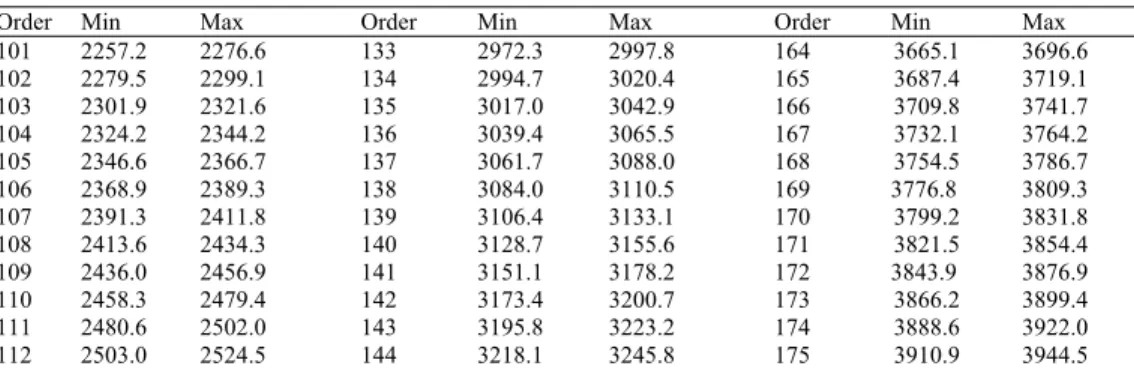
Table 1. Wavenumber boundaries (cm−1) of the diffraction orders; the first column is the
diffraction order number; the second and third columns are the average wavenumber of the first and last detector pixels.
Order Min Max Order Min Max Order Min Max 101 2257.2 2276.6 133 2972.3 2997.8 164 3665.1 3696.6 102 2279.5 2299.1 134 2994.7 3020.4 165 3687.4 3719.1 103 2301.9 2321.6 135 3017.0 3042.9 166 3709.8 3741.7 104 2324.2 2344.2 136 3039.4 3065.5 167 3732.1 3764.2 105 2346.6 2366.7 137 3061.7 3088.0 168 3754.5 3786.7 106 2368.9 2389.3 138 3084.0 3110.5 169 3776.8 3809.3 107 2391.3 2411.8 139 3106.4 3133.1 170 3799.2 3831.8 108 2413.6 2434.3 140 3128.7 3155.6 171 3821.5 3854.4 109 2436.0 2456.9 141 3151.1 3178.2 172 3843.9 3876.9 110 2458.3 2479.4 142 3173.4 3200.7 173 3866.2 3899.4 111 2480.6 2502.0 143 3195.8 3223.2 174 3888.6 3922.0 112 2503.0 2524.5 144 3218.1 3245.8 175 3910.9 3944.5
113 2525.3 2547.0 145 3240.5 3268.3 176 3933.3 3967.1 114 2547.7 2569.6 146 3262.8 3290.9 177 3955.6 3989.6 115 2570.0 2592.1 147 3285.2 3313.4 178 3978.0 4012.1 116 2592.4 2614.7 148 3307.5 3335.9 179 4000.3 4034.7 117 2614.7 2637.2 149 3329.9 3358.5 180 4022.7 4057.2 118 2637.1 2659.7 150 3352.2 3381.0 181 4045.0 4079.8 119 2659.4 2682.3 151 3374.6 3403.6 182 4067.4 4102.3 120 2681.8 2704.8 152 3396.9 3426.1 183 4089.7 4124.8 121 2704.1 2727.4 153 3419.3 3448.6 184 4112.1 4147.4 122 2726.5 2749.9 154 3441.6 3471.2 185 4134.4 4169.9 123 2748.8 2772.4 155 3464.0 3493.7 186 4156.8 4192.5 124 2771.2 2795.0 156 3486.3 3516.3 187 4179.1 4215.0 125 2793.5 2817.5 157 3508.7 3538.8 188 4201.5 4237.5 126 2815.9 2840.1 158 3531.0 3561.3 189 4223.8 4260.1 127 2838.2 2862.6 159 3553.4 3583.9 190 4246.2 4282.6 128 2860.6 2885.1 160 3575.7 3606.4 191 4268.5 4305.2 129 2882.9 2907.7 161 3598.1 3629.0 192 4290.8 4327.7 130 2905.3 2930.2 162 3620.4 3651.5 193 4313.2 4350.2 131 2927.6 2952.8 163 3642.8 3674.0 194 4335.5 4372.8 132 2950.0 2975.3
Table 2. Different binning options and size of the binned rows. Binning Option Number of binned
groups Number of rows in each bin Number of AOTF frequencies 16 2 16 4 12 2 12 4 4 8 4 1 3 8 3 1
4. Determination of the measurement altitude
The altitude of an observation corresponds to the tangent altitude, i.e. the distance from the planetary surface to the line of sight connecting the centre of the instrument entrance optics to the Sun, considering a 10’ depointing wrt the centre of the Sun. This depointing is introduced to ensure that the diffracted Sun remains within the slit for a longer period during the occultation. The tangent altitude is calculated for each bin by considering the centre of the corresponding slit portion. It is calculated from the spacecraft instantaneous position and orientation data, which are delivered as SPICE kernels [10]. The determination of the light path through the atmosphere, i.e. the path followed by the radiation reaching the instrument, requires that the planet’s curvature and atmospheric refraction be taken into account. The refraction model is based on the measurements performed during the Magellan mission [5].
Information about the measurement geometry, such as the tangent altitude, the measurement latitude, longitude, local solar time, angle of observation, distance of VEX to Venus, etc. are given at PSA Level 3 in the DATA folder together with the spectra.
5. Grating efficiency
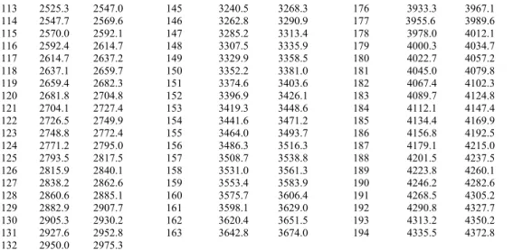
The Blaze function (BF) represents the efficiency of the grating in terms of refracted angle [11]. The efficiency is maximal when the refracted angle is equal to the incident angle. When the deviation between the angles increases, it is not the case anymore. The BF represents this effect and is calculated from the equations that can be found in [12, 13]:
(
)
(
)
(
)
(
)
2 2 2 1 cos cossin c sin sin
cos
cos 1 cos cos
sin c sin sin
cos cos sin sin cos B B B B B B B B if F if n σ γ α α β θ α β λ α β σ γ α α β θ α β α λ α λ α β σ γ α α θ ⋅ ⋅ ⋅ ⋅ + − ≥ = ⋅ ⋅ ⋅ ⋅ ⋅ + − < ⋅ = + ⋅ = + (1)
with λ the wavelength, σ the echelle groove spacing (250 μm), γ the angle between the incident ray and the plane perpendicular to the grooves which contains also the grating normal (2.60098°), α and β the incident and refracted angles to the grating plane, αB is the
angle between the incident ray and the facet normal in the plane perpendicular to the grooves (−0.019707°), θB is the Blaze angle (63.2°) and n is the diffraction order.
The function has lower values on the detector edge pixels compared to the detector central pixels (a maximum reduction of 10.5% is observed in order 101), and this effect increases when going to higher orders (up to a reduction of 26%), since dispersion increases for higher diffraction orders. The Blaze function has been computed for each pixel in all orders using Eq. (1) and is shown in Fig. 1. It is given in the archive at PSA Levels 2 and 3 in the files BLAZE.TAB under the CALIB directory.
Fig. 1. Blaze function intensity (gray scale), computed using Eq. (1), as a function of the diffraction order and the pixel number.
6. Determination of the transmittances and associated noise
Transmittances are calibrated spectra obtained by dividing each raw spectrum recorded during a solar occultation by a raw reference spectrum [5]. The latter is calculated from observations performed while looking at the Sun outside the atmosphere: it does not contain any information on the atmosphere itself. These exo-atmospheric raw spectra are measured either before the occultation in an ingress case, or after in an egress case. By dividing each occultation raw spectrum by this raw reference spectrum, all instrumental effects, such as ageing, are intrinsically removed. The raw reference spectra are, in fact, calculated by selecting a series of spectra recorded at tangent altitudes higher than 220 km (called zmax in
collected at altitudes lower than zmax are called atmospheric raw spectra. However the raw
reference spectra cannot simply be averaged because of small drifts in the exo-atmosphere raw signal value. A linear regression is performed on each of the 320 pixels as a function of time. For each atmospheric raw spectrum taken at a given time, an extrapolated reference spectrum is calculated taking into account the linear decrease (or increase) of the solar intensity (see [8] for more detail). A minimum of 40 spectra is always considered for the linear regressions. The 220 km altitude boundary zmax can be relaxed to lower altitudes if too
few raw spectra are measured at higher altitudes.
Transmittances are calculated for spectra from all measured bins and orders at tangent altitudes lower than zmax. In general the lowest altitudes reached are close to 60 km, which
correspond to zero transmittance spectra.
The noise levels are determined individually for each spectrum being part of one occultation, measured in each order and bin. A typical evolution of the signal on one pixel of the detector is given in Panel 1 of Fig. 2. This example corresponds to an egress: at the beginning no light reaches the detector as VEX is in the Umbra (U, in black, zoomed in Panel 3 of Fig. 2), then the occultation occurs when VEX in is the Penumbra (P, in red), and finally the instrument looks directly at the Sun and measures exo-atmospheric raw spectra (S, in blue, zoomed in Panel 2 of Fig. 2). The three zones used to derive the noise are in different colours in Fig. 2. The raw spectra can be considered as the sum of the measurement ( P ) and noise (δP), which contains all noise sources (photon noise, electronic noise, etc.). In the
following, the noise is assumed to be made of two components: a first term representing the electronic noise (constant for all spectra of one occultation), and a signal dependent term representative of the photon noise (only on S and P spectra, zero for U spectra). The noise δT
on the transmittance spectrum T on a particular pixel is calculated from the Umbra raw
spectrum U and the extrapolated raw reference spectrum S S= +0 α· t, as:
0 2 2 2 2 2 ( ) ( ) ( ) ( ) . ( ) ( ) ( ( ) ( ) ) T t S t S t S t S S t S P t P t P U U U P T t S T T T t P S P S P t S δ α δ δ δ δ δ δ δ δ = = + = + + = + = + + ⋅ ∂ ∂ = ∂ ⋅ +∂ ⋅ = (2)
where the noise levels in each zone (Sun, Penumbra and Umbra) are calculated as the standard deviation of the signal with time. In this relation, the noise from the Umbra spectra is the electronic noise. The noise during the Penumbra is obtained as
(
)
P U T S U
Fig. 2. Panel 1: Typical evolution through time of the signal (in ADU) on one pixel of the detector during a solar occultation. This example corresponds to an egress: at the beginning no light reaches the detector when VEX is in the Umbra (black line), then the occultation occurs when VEX in is the Penumbra (red line), and finally the instrument looks directly at the Sun and measures exo-atmospheric raw spectra (blue line). The exo-atmosphere and Umbra zones used to derive the noise are indicated by the boxes. Panels 2 and 3: Evolution of the variation of the noise signal around the mean value of the two zones (in ADU) exo-atmosphere in Panel 2 and Umbra in Panel 3. Standard deviation is shown by the lines in green.
The variations of the signals S(t) and U(t) around their respective mean values S and U
inside the exo-atmosphere and penumbra boxes shown in Panel 1 are also plotted for clarity in the expanded Panels 2 and 3 of Fig. 2. It can be seen that the mean value of the U signal is not zero, but is slightly shifted towards the negative values (in this particular example). This is probably due to an incorrect correction for non-linearity of the detector, since the SOIR detector response is non-linear at low signal levels [8]. The impact of this poor quality correction is 0.05 ADU for spectra having a low signal, as seen in Panel 3 of Fig. 3. It will only affect low intensity spectra, i.e. at the lowest altitudes, where the atmospheric lines are saturated.
Using Eq. (2) a noise pattern is built for each pixel of all spectra of the occultation. A typical example of such a noise pattern is presented in Fig. 3. It shows that the noise levels at the edges of the detector are larger, which is explained by the overall sensitivity of the instrument, mainly influenced by the Blaze function of the echelle grating.
We have found that the noise spectra associated with different observations vary considerably. Firstly, the noise level depends indirectly on the geometry of the observation through the time available to measure exo-atmospheric spectra before or after the occultation. This time is limited for solar occultations occurring at latitudes close to 60°N, due to spacecraft solar illumination restrictions. Secondly, it also depends on the measured diffraction order: the sensitivity of the detector is not the same at all wavenumbers [12] and the detector integration time has been optimized taking into account detector pixel saturation. The default integration time is 20 ms to avoid detector saturation, and it is set to 40 ms for orders 101 to 115 and 189 to 194 where the sensitivity is lower. And thirdly, it also depends on the value of the AOTF frequency imposed for the measurement, which changes the position of the maximum of the AOTF transfer function (see Section 9).
The noise levels are given in the archive at PSA Level 3 in the DATA directory together with the transmittance spectra.
Fig. 3. Transmittance (Panel 1) and associated noise (Panel 2) pattern for order 149 and bin 1 of orbit 341.1 for the altitude of 101 km as a function of the pixel number.
7. Spectral calibration
The pixel-to-wavenumber relation was previously obtained in [8] by considering about 100 well-defined solar lines in observations carried out outside the atmosphere. This spectral calibration resulted from the fitting of a polynomial between the wavenumber positions of these selected solar lines and the pixel position of the corresponding lines observed in different orders across the full wavenumber range. A polynomial of degree 3 was chosen for this calibration leading to an average error on the position of 30 other solar lines of about 0.05 cm−1. This spectral calibration is reported up to the version 3 of the SOIR PSA archive.
The general relations to calculate the wavenumber (ν) knowing a diffraction order (α), the pixel number (p) and the fourth order polynomial relation F(p) and its inverse function
F−1(ν/α) are
( )
1 F p p F ν α ν α − = ⋅ = (3)However, the spectral calibration varies slightly from spectrum to spectrum and from orbit to orbit, because of a Doppler shift induced by the change of speed of the VEX spacecraft projected on the line of sight and because of small changes in temperature inside the instrument during the measurement, which might induce misalignment of some optical elements. These temperature changes are partially measured by the thermal sensors inside the SOIR instrument, but are difficult to correlate with the observed variations of the spectral calibration.
To overcome this problem, we implemented a second calculation step in the spectral calibration on each spectrum, based on the presence of absorption lines with well -known positions in spectral databases such as HITRAN [14]. Pressure-induced line shifts were neglected since the resolution and the spectral sampling of SOIR are larger than the pressure shifts induced by collisions. The polynomial degree is five at maximum, though third degree polynomials are used in most of the cases. For some SOIR diffraction orders where few
absorption lines are present, the degree is set to lower values, depending on the number of spectral lines available for the calibration.
A new tool has thus been developed to automatically calibrate all spectra. This method relies on the pre-selection of well-defined absorption lines in each spectral interval. The selection is made manually on a series of selected spectra, chosen for their good signal to noise ratio and absorption well above the noise. The list of lines selected for calibration in one particular order is constructed by considering several criteria: well-defined and isolated lines, intense enough to be present on almost the complete set of spectra belonging to one occultation, lines coming from the central order or from the first adjacent ones, lines not perturbed by the noise (which is larger at the detector extremities, see Section 6). This list is then used in an automated way to calibrate all other spectra of all orbits recorded with the same settings (same order and same bin, see Table 2). The calibration results from the comparison of the observed positions of the selected lines and the positions found in spectroscopic databases. A spectral error is calculated for each spectrum by comparing the position of selected atmospheric lines in HITRAN and in the calibrated SOIR spectra. It varies from 0.005 to 0.02 cm−1.
Fig. 4. Example of spectrum recorded with the following settings: Orbit 116.1, Order 190, Binning option 12, Bin 1. Top: Observed (blue) spectrum with simulated spectrum (red) using the original pixel-wavenumber calibration using only solar lines. The red and blue crosses indicate the lines that are used to calculate the new calibration, and are linked in the Fig. with dashed black lines. Bottom: Same, but the simulated spectrum is using the new calibration based on the selection of the CO lines indicated in the Top Panel.
This calibration procedure will be illustrated by the following example: the order 190 is considered, which corresponds to the 4246.15 - 4282.62 cm−1 spectral interval. In this range,
CO is the main absorber, although absorption due to HF and HDO is also present. One band of CO is observed in the spectrum: the (2-0) band of the main isotopologue 12C16O (CO26,
using the HITRAN notation). Figure 4 illustrates the procedure on one such spectrum. In the top Panel, the observed spectrum is compared to the simulated one obtained by using the previous pixel-wavenumber relation whereas in the bottom Panel the calibration is based on the position of the CO selected lines, indicated with stars in the top Panel. This line information is reported in Table 3. Some of the lines used for the detailed calibration come from the orders adjacent to 190, order 191 in this particular case, because of orders superposition of adjacent ones on the detector. The quality of the spectral calibration is further illustrated in Fig. 5 where the root mean square (rms) values of the difference between
the positions of the selected lines in the calibrated SOIR spectra and HITRAN are plotted for each spectrum of one chosen occultation. In this case the rms value varies between 0.006 and 0.017 cm−1.
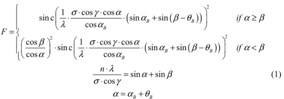
Table 3. List of CO lines used for the calibration of order 190. All lines belong to the main isotopologue and the (2-0) band. The position and the spectroscopic description of
the line are given. Some lines come from outside this order because of orders superposition.
Line SOIR measured position (cm−1) Coming from order
P 1 4256.22 190 P 2 4252.35 190 R 0 4263.83 190 R 1 4267.56 190 R 2 4271.16 190 R 3 4274.76 190 R 4 4278.24 190 R 4 4278.23 191 R 5 4281.66 191 R 6 4285.01 191
Fig. 5. Evolution of the rms values between the positions of the lines selected for calibration in the SOIR spectra and in HITRAN for the occultation observation during orbit 116.1 (Order 190 – Bin 1).
The same procedure is then applied automatically to the other spectra of the complete occultation. Indeed as the signal degrades (at higher altitudes, the absorption lines are just above or within the noise and at lower altitudes, the signal weakens due to light absorption by aerosols in the Venus atmosphere), fewer lines can be used for calibration and it deteriorates. The automatic procedure detects when the calibration is starting to deteriorate (either the number of usable lines is too low, or the regression between observed and HITRAN positions is too poor). Calibration for such spectra is then the same as the one determined for the closest spectrum for which the calibration was deemed acceptable.
The direct calibration F(p) is reported in the archive at PSA level 3 in the DATA directory together with the spectra. The inverse relation is not given since it can easily be calculated from the direct one.
8. Determination of the spectral resolution
The determination of the resolution of the SOIR instrument has been completely reassessed since the first results published in [8]. In that paper, resolution, defined as the FWHM of a
sinc2 function, was obtained by considering a limited number of solar lines. A new method
has been developed relying on atmospheric absorption lines rather than solar lines. The same lines as those selected for the calibration in each individual order (see Section 7) are also used for the determination of the resolution. Gaussian profiles representing the Instrument Line Function (ILS) of the instrument are now used instead of a sinc2 function. This choice was
based on the observation that using a sinc2 function introduced side lobes that were not
present in the SOIR spectra. A Gaussian profile is fitted to each of these selected lines and the FWHM width is extracted. Indeed, the width of a line is imposed by the instrument spectral resolution. As an example, the FWMH value at infinite resolution of the R7 line of the (2-0) band of CO at 4288.29 cm−1, corresponding to a temperature of 200 K and a pressure of 10
mbar is 0.00935 cm−1, almost 20 times narrower than the SOIR resolution in that order (0.2
cm−1).
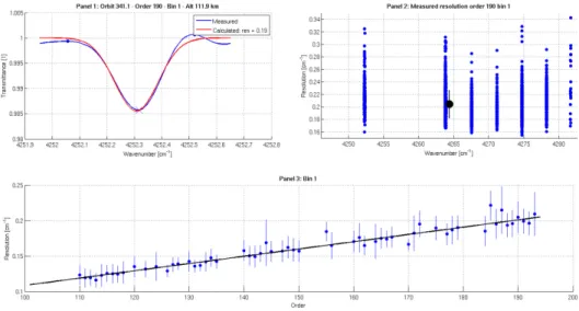
Typical results of this fitting procedure are presented in Fig. 6. An observed line and its corresponding Gaussian profile are shown in Panel 1. Panel 2 shows the individual FHWM obtained using this method for order 190 (bin 1), considering a large series of orbits and different altitudes. The high variability of the results originates from the noise, and the fact that a line is only defined on a few pixels. For each order (and bin), a mean value is obtained along with a standard deviation. The resolution over the complete SOIR spectral range is then modelled by a polynomial of degree 1 passing through all the individual values weighted by the standard deviations. This polynomial is the following (Binning 12 option):
1 3 3 1 1 3 3 2 1.0266 10 5.8760 10 1.0596 10 4.7473 10 bin bin Res cm x x Res cm x x α α − − − − − − = + = + (4)
where α is the order number and Res is the resolution. Panel 3 summarizes the results of this analysis. The individual points are the resolution values obtained in each order; the error bars represent their standard deviation. The modelled resolution is shown as the black line.
Fig. 6. Panel 1: Examples of fitting the Gaussian ILS on one individual well-defined CO line in order 190 (bin 1). Panel 2: Individual FHWM widths fitted on atmospheric absorption lines for order 190 and bin 1 from all the available orbits. The mean value and standard deviation are also shown as the black point. Panel 3: Resolution on the complete spectral range of the SOIR instrument, where the individual points are the values of the resolution in the different order and the error bars represent the standard deviation in each order. The best polynomial fit (degree 1) is shown in black.
The resolution value for each order can be found in the SOIR archive at Levels 2 and 3 in the RESOL_BINNINGXX.TAB files under the CALIB directory, where XX corresponds to the binning case (see Table 2).
9. Characterization of the AOTF
The AOTF filter is the central element of the SOIR instrument in the sense that it selects which spectral interval will be recorded: being wanted (from the selected order) or undesired (from adjacent orders). The determination of its characteristics is therefore essential. Two quantities are needed to fully describe the response of the AOTF: its tuning function and its transfer function. The tuning function gives the relation between the AOTF radio frequency applied to the crystal and the central wavenumber passing through the filter. The second function indicates how the different components of an incident light signal are transferred through the crystal. Several studies have already been performed on both functions [8, 9, 12]. Their results are summarized here below.
9.1. Transfer function
The theoretical representation of the AOTF transfer function is a sinc2 function:
( )
2 0 . sin 0.886. AOTF I c fwhm ν ν ν = − (5)where I is the intensity at the centre, ν is the wavenumber, ν0 is the central wavenumber and fwhm is the full width half maximum of the function. The use of such a simple expression has
been shown to be insufficient in the case of the SOIR instrument, for which the AOTF function is highly asymmetric. A method was proposed to simulate the transfer function by a sum of five sinc2, allowing for asymmetry [9]:
( )
2 2 0 2 . sin 0.886. i i i i AOTF I c fwhm ν ν ν =− − =
(6)where Ii are the intensity coefficients, ν0i the wavenumber position of the maximum of the
sinc2 functions, and i
fwhm the full width half maximum of each sinc2 function.
Moreover it was shown that the AOTF transfer function varied a lot within the spectral range covered by SOIR. Therefore, the parameters appearing in the five sinc2 functions were
derived taking into account a first order wavenumber dependency. This had to be done for each binning option defined in Table 2.
In practice, due to the high variability of the transfer function, this was still not enough to reproduce the AOTF function satisfactorily for each setting. We decided to determine the function separately for each setting directly from the observed spectra and, where possible, over the equivalent spectral width of at least five adjacent orders and use these individual functions instead. These functions correspond to the first step in the analysis presented in [9] (see Fig. 7 in [9] as an example of such results).
The AOTF transfer function values for each order can be found in the SOIR archive at Levels 2 and 3 in the AOTF_TF_BINNINGXX.TAB files under the CALIB directory, where XX corresponds to the binning case (see Table 2).
9.2. Tuning function
The tuning function describes the relation between the frequency applied to the AOTF crystal and the wavenumber corresponding to the maximum of the signal transferred through the crystal. The method used to obtain this relation has been explained in full detail in [12]. No
major improvements have occurred since. For each setting (binning option/bin) two relations of the type:
(
)
(
)
2 1 2 . . . . TF f a b f c f TF f ν ν α β ν γ ν − → + + → + + = = (7)have been derived. The tuning function polynomial coefficients can be found in the SOIR archive at Levels 2 and 3 in the AOTF_F_WN.TAB files under the CALIB directory.
10. Description of the archived data
The SOIR PSA archive can be found on the ESA servers at the address http://www.rssd.esa.int/index.php?project=PSA&page=vex. This paper describes the Version 4.0 of the SOIR archive, which corresponds to Release 3 and Revision 0. The format has changed significantly compared to previous versions.
The observations are separated in data sets at PSA Levels 2 and 3 as a function of the mission extension during which they were recorded: the nominal mission covers observations up to orbit 530, the first extension up to orbit 1136, the second extension up to orbit 1584, the third extension up to orbit 2080 and the fourth one for the latest orbits.
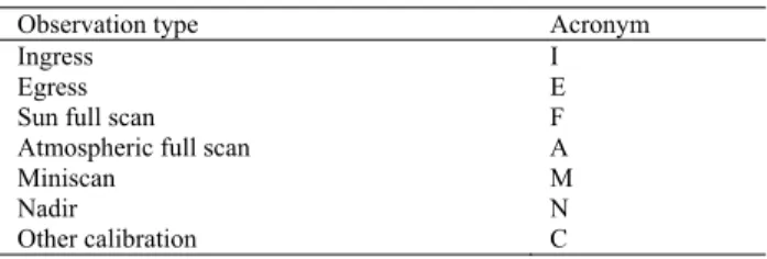
The name of an observation is based on the date it was recorded and its type. Because the orbital period of VEX is 24 hours, different measurements can be done during one day, for example an ingress followed by an egress. The format is YYYYMMDD_TCC where YYYY is the year of the orbit, MM is the month, DD is the day, T is the type of measurement and CC is the measurement number during that orbit, starting from 1. The types of observations are summarized in Table 4. Besides egresses and ingresses, which correspond to solar occultation observations carried out when exiting or entering penumbra, there are also Sun and atmospheric full scans (all orders are scanned sequentially), mini-scans (the AOTF frequency is scanned over a short interval) and nadir (looking at the surface of the planet). Only ingresses and egresses are given in the archive at PSA Level 3.
Table 4. Types of SOIR observations Observation type Acronym
Ingress I Egress E Sun full scan F
Atmospheric full scan A
Miniscan M Nadir N Other calibration C
We will briefly describe the files making up the Level 3 PSA archive, with special emphasis on the calibration (CALIB directory) and spectra files (DATA directory). Indeed the complete archive contains a lot of files describing the formats, the content, retracing the history of the archive. They can be found under the DOCUMENT and CATALOG folders. The archive BROWSE directory contains spectra Figs. in JPG format: the sum of all pixels as a function of time at PSA Level 2, and all the transmittance spectra at PSA Level 3. We will only explain how the different calibrations and the instrument characterization are implemented in the archive. All the ASCII data are given in TAB files. They are accompanied by LBL files, which describe the content of the data files.
All calibration files can be found under the CALIB directory at PSA Levels 2 and 3. Several files can be found concerning:
(1) The resolution file (RESOL_BINNINGXX.TAB, with XX the binning option) contains the values of the resolution (FWHM of a Gaussian ILS) for each diffraction order and bin;
(2) The AOTF tuning function file (AOTF_F_WN.TAB) contains the values of the parameters converting AOTF frequency into diffraction order central wavenumber, and vice-versa;
(3) Files containing the AOTF transfer function (AOTF_TF_BINNINGXX.TAB, with XX the binning option): one file per binning option. For example, the file AOTF_TF_BINNING12.TAB contains the 94 transfer functions for all orders from 101 to 194 for bins 1 and 2. The function is given on a fixed wavenumber scale defined by 3 parameters (starting wavenumber, step and number of points);
(4) The blaze function for each order (BLAZE.TAB file).
The files containing the SOIR spectra are given in the DATA directory, one observation in one individual directory having the name described above (YYYMMDD_TCC). The spectra are in the files YYYYMMDD_TCC_OOO.TAB, where OOO is the order selected. One line of such a file contains the information on one spectrum of one particular bin (for example, for the binning option ’12’, there are 2 lines, one for each bin). For each bin, the corrected transmittance, the noise and the polynomial coefficients to calculate the calibrated wavenumber scale are given. The polynomial to calculate the wavenumber scale corresponds to the analysis described in this study (see Section 0). A series of parameters describing the observation are also given, including the date and time, the position of the satellite and viewing geometry. All parameters needed for the interpretation of the spectra are included. Some housekeeping parameters are also provided to follow the status of the instrument during the occultation.
11. Conclusions
We have presented several improvements in the calibration and characterization of the SOIR instrument introduced in the data pipeline since [8]. They concern mainly the spectral calibration which has been improved by not only considering solar lines but also atmospheric absorption lines in each individual order of the instrument. The characterization of the ILS has also improved by considering a large number of atmospheric lines compared to the limited number of solar lines that were previously used for this purpose. The detailed investigation of the noise on each individual pixel has led to the determination of noise spectra defined for each spectrum, as it was shown that this noise pattern was highly dependent on the observation settings. We have also described the data archive for the SOIR instrument, describing what information should be found in which file. We believe that this paper, along with the archived data, allow the potential user to take full advantage of the richness of the SOIR spectra. We encourage users to make use of the archived spectra and data.
Acknowledgments
The research program was supported by the Belgian Federal Science Policy Office and the European Space Agency (ESA – PRODEX program – contracts C 90323, 90113, and C4000107727). The research was performed as part of the “Interuniversity Attraction Poles” programme financed by the Belgian government (Planet TOPERS).