HAL Id: insu-01164292
https://hal-insu.archives-ouvertes.fr/insu-01164292
Submitted on 4 Mar 2021HAL is a multi-disciplinary open access archive for the deposit and dissemination of sci-entific research documents, whether they are pub-lished or not. The documents may come from teaching and research institutions in France or abroad, or from public or private research centers.
L’archive ouverte pluridisciplinaire HAL, est destinée au dépôt et à la diffusion de documents scientifiques de niveau recherche, publiés ou non, émanant des établissements d’enseignement et de recherche français ou étrangers, des laboratoires publics ou privés.
Coordinated Hubble Space Telescope and Venus Express
Observations of Venus’ upper cloud deck
Kandis Lea Jessup, Emmanuel Marcq, Franklin Mills, Arnaud Mahieux,
Sanjay Limaye, Colin Wilson, Mark Allen, Jean-Loup Bertaux, Wojciech
Markiewicz, Tony Roman, et al.
To cite this version:
Kandis Lea Jessup, Emmanuel Marcq, Franklin Mills, Arnaud Mahieux, Sanjay Limaye, et al.. Coor-dinated Hubble Space Telescope and Venus Express Observations of Venus’ upper cloud deck. Icarus, Elsevier, 2015, 258, pp.309-336. �10.1016/j.icarus.2015.05.027�. �insu-01164292�
Coordinated Hubble Space Telescope and Venus Express Observations of Venus’ upper cloud deck
Authors: Kandis Lea Jessup1,3, Emmanuel Marcq2, Franklin Mills3,10, Arnaud Mahieux4 , Sanjay Limaye5 , Colin Wilson6 , Mark Allen7, Jean -Loup Bertaux2, Wojciech
Markiewicz8, Tony Roman9 , Ann-Carine Vandaele4, Valerie Wilquet4 , Yuk Yung8
Southwest Research Institute, 1050 Walnut Street, Boulder CO 80302, USA1Université de Versailles Saint-Quentin – Laboratoire LATMOS, 11 boulevard
d'Alembert, 78280 Guyancourt. France2
Research School of Physics and Engineering and Fenner School of Environment and Society, the Australian National University, Canberra, ACT 02003
Belgian Institute for Space Aeronomy, Avenue Circulaire, 3, B-1180 Brussels, Belgium4
University of Wisconsin, Atmospheric Oceanic &Space Science Department, 1225 W Dayton St Madison WI, 53706 USA5
Oxford University, Oxford, UK6
Caltech, 1200 E California Blvd Pasadena, CA, 91125, USA8
Max Planck Institute for Solar System Research, Justus-von-Liebig-Weg 3, 37077 Göttingen, Germany7
Space Telescope Science Institute, 3700 San Martin Drive Baltimore MD 21218, USA9
Space Science Institute, 4750 Walnut St #205, Boulder CO 80301, USA10
Pages: 54 (1.5 spaced, including 5 pages of references) Figures: 19
Abstract: Hubble Space Telescope Imaging Spectrograph (HST/STIS) UV observations of Venus’ upper cloud tops were obtained between 20N and 40S latitude on December 28, 2010; January 22, 2011 and January 27, 2011 in coordination with the Venus Express (VEx) mission. The high spectral (0.27 nm) and spatial (40-60 km/pixel) resolution HST/STIS data provide the first direct and simultaneous record of the
latitude and local time distribution of Venus’ 70-80 km SO and SO2 (SOX) gas density on Venus’ morning
quadrant. These data were obtained simultaneously with a) VEx/SOIR occultation and/or ground-based James Clerk Maxwell Telescope sub-mm observations that record respectively, Venus’ near-terminator
SO2 and dayside SOx vertical profiles between ~75-100 km; and b) 0.36 µm VEx/VMC images of Venus’
cloud-tops. Updating the (Marcq, E., Belyaev, B., Montemssin, F., Fedoroav, A., Bertuax, J-L., Vandaele,
A. C., Neefs, E. [2011], Icarus, 211: p. 58–69) radiative transfer model SO2 gas column densities of ~ 2-10
µm-atm and ~ 0.4-1.8 µm-atm are retrieved from the December 2010 and January 2011 HST observations,
respectively on Venus’ dayside (i.e., at Solar Zenith Angles (SZA) < 60°); SO gas column densities of
0.1-0.11µm-atm, 0.03-0.31 µm-atm and 0.01-0.13 µm-atm are also retrieved from the respective December 28,
2010, January 22, 2011 and January 27, 2011 HST observations. A decline in the observed low-latitude
0.24 and 0.36 µm cloud top brightness also paralleled the declining SOx gas densities. On December 28,
2010 SO2 VMR values ~ 280-290 ppb are retrieved between 74-81 km from the HST and SOIR data
obtained near Venus’ morning terminator (at SZAs equal to 70° and 90°, respectively); these values are 10x
higher than the HST-retrieved January 2011 near terminator values. Thus, the cloud top SO2 gas abundance
declined at all local times between the three HST observing dates. On all dates the average dayside SO2/SO
ratio inferred from HST between 70-80 km is higher than that inferred from the sub-mm the JCMT data
above 84 km confirming that SOx photolysis is more efficient at higher altitudes. The direct correlation of
the SOx gases provides the first clear evidence that SOx photolysis is not the only source for Venus’ 70-80
km sulfur reservoir. The cloud top SO2 gas density is dependent in part on the vertical transport of the gas
from the lower atmosphere; and the 0.24 µm cloud top brightness levels are linked to the density of the
sub-micron haze. Thus, the new results may also suggest a correlation between Venus’ cloud-top sub-sub-micron haze density and the vertical transport rate. These new results must be considered in models designed to
simulate and explore the relationship between Venus’ sulfur chemistry cycle, H2SO4 cloud formation rate
and climate evolution. Additionally, we present the first photochemical model that uniquely tracks the
transition of the SO2 atmosphere from steady to non-steady state with increasing SZA, as function of
altitude within Venus’ mesosphere, showing the photochemical and dynamical basis for the factor of ~2
enhancements in the SOx gas densities also observed by HST near the terminator above that observed at
smaller SZA. These results must also be considered when modeling the long-term evolution of Venus’ atmospheric chemistry and dynamics.
Keywords: Venus; Venus, atmosphere; Atmospheres, composition; Atmospheres, chemistry
1. Introduction and Overview
Venus’ atmosphere is known to be composed predominantly of carbon dioxide (total volume mixing ratio of 0.965) and nitrogen gas, where the latter is a distant second to the former. Although sulfur oxide gases and aerosols are only trace components of Venus’ atmosphere, chemical reactions in Venus’ atmosphere that involve these species such as SO2, SO, OCS, and H2SO4, are important because they are closely linked to the global-scale H2SO4 cloud and haze layers located at altitudes between 30-100 km (Fig. 1). Additionally, though volcanic activity has yet to be directly observed on Venus, detailed thermochemical modeling of Venus’ near surface chemical make-up indicates that volcanic outgassing is the most probable source atmospheric sulfur in Venus’ lower atmosphere (i.e. below 60 km) (Johnson and Fegley 2002).
Notably, Venus’ 60-100 km altitude region was extensively observed during the time period extending from the late 1970s to early 1990s and during the Venus Express (VEx) mission (2006-2014). Likewise, extensive modeling of the dynamics and chemistry of Venus’ atmosphere (e.g., Krasnopolsky and Pollack 1994, Krasnopolsky 2007) has been on-going. Yet, the mechanism(s) that control the exchange of SO2 between the lower atmosphere and the mesosphere are not fully understood. Some recent modeling efforts have considered whether the vertical transport of the gas to the mesosphere occurs in conjunction with Hadley cell circulation (Yung et al 2009, Marcq et al. 2013); while previous observers have suggested that direct volcanic ejection (Esposito et al 1988) may be a key mechanism for the exchange of the gas from the troposphere (z < 60 km) to the mesosphere (~ 60-90 km, see Clancy et al. 2003, Betraux et al. 2007). The biggest challenge to understanding how the exchange occurs is the fact that portions of the lower atmospheric region are statically stable. Suppression of this stability due to changes in the vertical temperature profile may help promote the vertical transport of sulfur, and other processes such as small scale eddies, and or adsorption/desorption on cloud particles (just to name a few) may also contribute to the vertical transport of sulfur in Venus’ atmosphere. Because the exact mechanism for the vertical transport of sulfur is unknown sulfur oxide observations are highly prized since they provide the data needed to properly assess the ongoing chemical evolution of Venus’
atmosphere, atmospheric dynamics, and could even provide insight into the nature and frequency of volcanism on Venus.
Consequently, a vast suite of SO2 and SO observations were obtained in conjunction with the VEx mission (e.g., Sandor et al 2010, Belyaev et al 2012, Marcq et al 2011) in order to probe the 60-100 km altitude region of Venus’ atmosphere using both Earth-based telescopes and VEx instrumentation. These observations have revealed unexpected spatial patterns and spatial/temporal variability that have not been satisfactorily explained by models (Zhang et al 2012, Krasnopolsky 2012). For example, high (≥ 400 ppb) SO2 abundances were observed within the mesosphere in 2007 (Belyaev et al 2012, Marcq et al 2011), and an on-going decline in the SO2 abundance was consistently observed throughout the remainder of the VEx mission (Marcq et al. 2013, Marcq pers. communication) [Fig. 2]. Venus’ long-term (i.e., from ~1980 to 2014) mesospheric SO2 abundance record suggests this behavior may be cyclical in nature (Marcq et al 2013); if so, the observed behavior cannot be explained as a function of local time variations but may be an indication of active volcanism. Of equal intrigue is the equator-to-pole SO2 abundance gradient, which seems to be typically increasing towards the equator, but can also show the opposite trend (Marcq et al. 2013). The mechanism that causes the observed latitudinal gradient to change slope is not fully understood, but seems to be connected with low levels of SO2 gas abundance, and may be connected to changes in the convective mixing intensity (c.f. Marcq et al. 2013).
In December 2010 and January 2011 170-310 nm, high spectral (0.3 nm) and spatial (40-60 km/pixel) resolution observations of Venus’ low latitude dayside atmosphere were obtained using Hubble’s Space Telescope Imaging Spectrograph (the HST/STIS). These observations probe the SO2 and SO gas absorption signature in Venus’ ~ 65-80 km region and were obtained in coordination with (a) low latitude Venus Express Monitoring Camera (VMC) cloud top imaging; (b) solar occultation SO2 spectroscopy obtained using the VEx Solar Occultation in the Infrared (VEx/SOIR), (Belyaev et al. 2012); (c) and ground-based sub-mm measurements of Venus’s average dayside SO and SO2 gas densities between 70-100 km obtained using the James Clerk Maxwell Telescope (JCMT) (Sandor et al. 2010). The acquired HST/STIS data also serve as a complement to the high-spatial, low-spectral (1.5 nm) resolution nadir viewing spectra obtained using
the VEx Spectroscopy for Investigation of Characteristics of the Atmosphere of Venus (VEx/SPICAV) (Macrq et al. 2013) throughout the lifetime of the Venus Express mission. The primary objective of the coordinated observing effort was to obtain detailed information on the horizontal distribution of the SO2 and SO gas density in the 65-80 km region, while a) simultaneously obtaining information on the vertical distribution of the gases between 65-100 km; and b) collecting information on the cloud top brightness levels in the regions that are spatially co-located with the SO2 and SO gas density measurements. These types of data are needed to develop observationally informed models that are able to simulate and explore the photochemical, dynamical and radiative processes responsible for Venus’ atmospheric evolution.
2. Observation Description
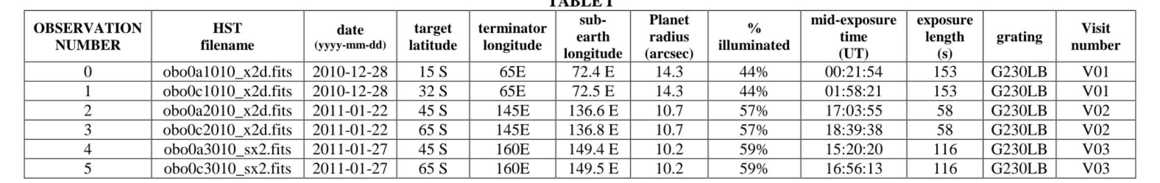
The first (and thus far only) HST/STIS observations of Venus’ upper cloud deck were obtained on 3 dates in December 2010 and January 2011 using the G230LB (170-317 nm) grating, with the 52″x0.1″ slit and the CCD detector (0.51" pixels), to obtain high spectral (0.27 nm) and spatial (40-60 km/pixel, assuming 2 pixel binning) resolution measurements of Venus’ SO2 and SO gas absorption signatures [Fig. 3]. The specific dates of observation were December 28, 2010; January 22, 2011; and, January 27, 2011. On each date (or “visit” to Venus) Venus was observed with the 52" HST/STIS slit centered on the morning terminator longitude, so that Venus’ morning quadrant was observed from the terminator to the sunlit limb. For our chosen dates the observable sunlit quadrant corresponded to ~12-18" of daylight, covering ~ 90-121o E. longitude. And, on each date Venus was observed with the HST/STIS slit in its nominal 45o orientation. In this orientation, a different time of day and latitude was recorded in each pixel. In order to build up a picture of the SO2 and SO gas absorption signatures as a function of time of day at multiple latitudes, two exposures were taken on each visit, and in each exposure the center of the 52" slit intersects the morning terminator longitude at a single unique latitude [Fig. 4, Table I].
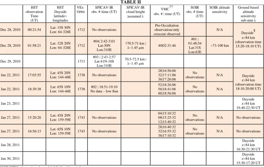
On each date, the data were obtained simultaneously and/or contemporaneously with ground-based sub-mm spectral observations of Venus and UV-Visible imaging of Venus’ atmosphere obtained by the VEx/VMC and VEx/VIRTIS (Visible and Infrared
Thermal Imaging Spectrometer) or near infrared spectral observations obtained with the VEx/SOIR instrument (see Table II). Additionally, our observing program was designed to align with the planned coordinated VEx and JAXA launched Venus Climate Orbiter (VCO, also known as Akatsuki) imaging of Venus’ cloud tops—thus imaging from both an equatorial and pole-centered view would have been simultaneously obtained with the spectral observations. As alluded to above, the primary objective of the coordinated observing effort was to obtain detailed information on the horizontal distribution of Venus’ cloud top SO and SO2 gas abundance distribution (in terms of latitude, longitude and time of day), while simultaneously obtaining information on the vertical distribution of the gases between 65-100 km, as well as collecting information on the cloud contrast and/or brightness in the regions that were spatially co-located with the SO2 and SO gas density measurements. Although VCO was not able to successfully insert into Venus Orbit in December 2010, the coordinated VEx and earth based observing effort was executed.
Thus, on December 28, 2010, VEx/SOIR 4 µm solar occultation spectra of Venus’ mesosphere were obtained along the Earth-facing morning terminator at 2 UT at an impact (or target) latitude of 30.68S [Fig. 5]. In coordination with the VEx/SOIR observations, HST/STIS observations of Venus that recorded Venus’ dayside 170-310 nm UV signature from noon to the Earth-facing morning terminator were obtained within the 0-2 UT time period. In the first exposure [OBS 0] the target latitude along the Earth facing terminator was defined to be 15S latitude. In the second exposure [OBS 1], taken simultaneously with the VEx/SOIR occultation observations, the target latitude at the terminator was set at 32±2 S latitude in order to match the target latitude of the VEx/SOIR solar occultation observations. In conjunction with the SOIR observations, observations of Venus’ airglow were obtained by Venus Express using the VIRTIS-M instrument, which covers the near-UV and visible wavelengths from 0.25-1.0 µm. However, these observations focused on the nightside near the anti-solar point. While these observations can provide data needed to better understand the day vs. night oxygen abundances on Venus, an in-depth discussion of the implications of the nightside VIRTIS data relative to the morning quadrant HST observations is beyond the scope of this paper.
On January 22 and 27, 2011 VCO would have been at an optimal position to obtain UV images of the Venus cloud tops on the dayside hemisphere observable from Earth-based telescopes in the time period extending from 13:00-19:00 UT. At the same time, the orbital phases of VCO and VEx would have been coincident. Therefore, VEx scheduled and acquired successive UV images of Venus’ cloud tops using the VEx/VMC camera that could be used to calibrate and validate the planned VCO imaging sequence. As a complement to those observations, HST/STIS observations were obtained on each of these dates in the 15-18 UT time period. As discussed above, two HST/STIS exposures (OBS 2 & OBS 3 on January 22 and OBS 4 & OBS 5 on January 27) were obtained per day of observation. For each of these dates, the slit was centered at the morning terminator at 45S in the first exposure and at 65S in the second exposure [Fig. 4]. Given the 45° orientation of the slit, this resulted in the dayside coverage along the slit extending from high latitudes at the terminator to low latitudes at the sunlit limb [Fig. 4]. Because of the overlap in the time signature of the VMC imaging and the HST spectral observations, the SO2 gas density signature recorded in the HST spectra can be directly mapped to the cloud patterns captured in the field of view of the available VEx VMC images between 17-19 UT on January 22 and between 15-17 UT on January 27 [Fig. 5]. Additionally, because the HST/STIS observations were obtained in the exact same observing geometry on each of these dates, variability in the gas behaviour at each latitude and time of day was recorded at the cadence of Venus’ 5 “day” cloud top rotation period. I.e., Titov et al. 2012 reports the cloud top zonal wind-speed to be 0.09 km/s at latitudes ±45° from the equator; similarly, measurements provided by Khatuntsev et al. (2013) that bracket the time period of the coordinated observations show that the cloud top zonal wind speed was primarily ~ 0.085-0.095 km/s, for an average zonal cloud top wind speed of 0.09 km/s. Given Venus’ 6051 km radius it takes 4.89 Earth days to traverse Venus’ circumference. The January 27 observations of Venus’ cloud tops were obtained 4.92 Earth days subsequent to the January 22 observations, thus matching near exactly the expected equatorial cloud rotation period.
Based on the acquired HST/STIS observations we provide in Section 5 a detailed description of the SO2 and SO gas density variation as function of latitude and time of day for each of these dates. A description of the data calibration steps and the gas density
retrieval methods is provided in Sections 3 and 4, respectively. And a detailed comparison of the HST results to the observations obtained contemporaneously by VEx as well as other ground-based observers is provided in Section 6
3. Data Reduction
3.1Flux Calibration: The HST/STIS observations were initially reduced using the Space Telescope Science Data Analysis System (STDAS) CALSTIS, i.e., the STIS calibration and reduction pipeline which handles flat-fielding, geometric rectification, bias and dark subtraction. However, the pipeline reduced spectra still retained some level of residual flux from the sky. Because the observations were obtained with the 52” long slit, the sky background could be straightforwardly estimated from the flux levels recorded in regions of the slit sufficiently far from the edge of Venus’ 22±2" disk diameter. This value was then subtracted from the observed flux at all wavelengths.
Although HST/STIS has a solar blind Multi-Anode Microchannel Array (MAMA) detector, the UV flux from Venus would have exceeded the brightness levels of that detector. Consequently, in order to obtain high signal-to-noise (S/N) observations of Venus within the limited time period allotted for Venus observations, the exposures had to be obtained using the CCD detector and the G230LB grating, which is known to produce strong grating scattered light below 230 nm at wavelengths where the CCD detector has a high sensitivity. Fortunately, the grating scattered light levels can also be estimated directly from the observed spectra. The G230LB grating disperses light throughout the 170-320 nm region, but the solar flux becomes very weak below 200 nm – dropping by 3 orders of magnitude between 300 and 170 nm – and the expected signal from Venus below 190 nm is basically zero because of the strong CO2 absorption below 200 nm. I.e., at 190 nm only about 1% of incident solar flux is scattered back to the Earth from the cloud tops and that flux levels is about a factor of 2 below the 190 nm detection limit of the instrument when using G230LB grating in concert with the CCD detection; it is also a factor of 10 below the detection limit needed at 170 nm. Consequently, any flux detected at wavelengths < 190 nm will be due to grating scattered light. Therefore, we used the flux levels detected at 185±5 nm to estimate the level of grating scattered light in
the observed spectra and subtract off this residual flux from the observations at all wavelengths.
In each of these cases, to make the necessary corrections we first converted the calibrated flux defined per pixel in units of erg/s/Å/cm2/arcsec2 to count rates based on the HST provided detector sensitivity levels per wavelength. Once the sky background and the grating scattered light levels were estimated in count units and subtracted off from the raw flux defined in count units, the observed flux was then returned to the calibrated flux units.
The CCD detector is also very sensitive to cosmic rays. Though the exposure times used for our observations are relatively short (~0.5-2.5 min) the 2-D (1024 spatial-pixel x 1024 spectral-spatial-pixel) spectral maps recorded by HST/STIS are riddled with cosmic rays. I.e., out of the 785 spectral pixels included in each spectrum above 200 nm, there were ~ 5±5 spectral pixels that were impacted by cosmic rays per spatial pixel. Since Venus had not been observed by HST/STIS before, we opted to complete the cosmic ray correction of the data subsequent to the pipeline reduction of the data. Utilizing the corrected flux defined in count units, we removed the cosmic-rays from the spectral maps by comparing the count rate detected per spatial and spectral pixel with the median count rate detected within a 10 spatial pixel range, and replaced any high (more than 30x greater) count rates with the lower median value.
3.2 Wavelength Calibration: Analysis of the gas absorption signatures included in the Venus flux spectra was completed based on the ratio of the fully calibrated and corrected flux to a well calibrated solar spectrum. Consequently, although the initial pipeline reduction includes an approximate wavelength calibration, careful assessment of the absolute wavelength assignment per pixel post-pipeline reduction was needed to ensure alignment with the chosen solar spectrum. Because the variability of the highly structured solar spectrum at UV wavelengths can be significant, it was imperative that we utilize contemporaneously obtained solar spectra in the reduction of the HST acquired Venus spectra (McClintock et al. 2005, Egorova et al. 2008). We utilized the solar flux measured by SOLSTICE at (0.033 nm sampling, 0.1 nm FWHM) on each of the 6 dates of observation (Marty Snow, personal communication). To accurately align the solar spectrum and the observed Venus flux we re-sampled the SOLSTICE spectra to match
the STIS data. In particular, the HST/STIS 0.1” slit and the G230LB grating (1.35 Å/pixel dispersion) with the CCD detector (which has 0.051”x0.051” pixels) produces data with a spectral resolution of 0.27 nm full width half maximum (FWHM) [Fig. 3]. Therefore, we convolved the SOLSTICE spectra with a Gaussian comparable to the complex 0.27 nm line-spread function (LSF) profile expected from the convolution of the STIS point-spread function (Woodgate 1998) with the 0.1” slit. We made small corrections to the wavelength of each STIS spectrum by aligning the Fraunhofer absorption lines with those in the solar spectrum. We found that adjustments of 0.09 nm or less (which is less than one-third of the FWHM) were required to achieve alignment with the solar spectrum. This step is a key safeguard against the introduction of artifacts into the reflectance spectra which is defined as a function of the ratio of the observed spectrum and the solar spectrum (see below for the complete definition of the reflectance spectrum).
3.3 Assignment of Spatial Coordinates per pixel: In order to assign the exact latitude, longitude, and time of day value to each spatial pixel we first generated a 2-D disk with a plate scale equivalent to the HST/STIS pixel size that is representative of the projection of Venus’ Earth-facing disk on the sky. Based on this disk the latitude and longitude values at each point of the disk can be defined based on Venus’ angular diameter on the date of observation and the known Venus North pole position angle. Likewise, we can project a 2-D representation of the slit across that disk based on the known Venus North pole position angle, the known HST/STIS spatial pixel size, the slit orientation relative to the North pole position angle and the target latitude and longitude of the center of the HST/STIS slit. Based on the intersection of that slit projection with the observable regions of Venus’ Earth facing disk, the exact latitude, longitude, and time of day intercepted at each pixel along the length of the slit is defined. The accuracy of the latitude, longitude, and time of day assignments are thus dependent on accurate intersection of the center of the HST/STIS slit with the target latitude and longitude. To accommodate for any offsets between the targeted latitude and longitude and the observed latitude and longitude, we first identified the initial on-disk pixel value evidenced by the spatial profile produced by the observed flux and then adjusted the pixel assigned to the target longitude to the correspond to the value expected from the known
geometry of the slit and the known radial extent of Venus’ disk per date of observation. Because neither HST nor VEX obtained full disk images of Venus, the spatial profiles recorded in the HST/STIS slit could not be directly compared with a model profile derived from the disk image. Fortunately, the expected uncertainty in the HST/STIS targeting is ~0.01 arcsec (0.2 spatial pixel or ~ 5 km).
3.4 Spatial Binning: Once the latitude and longitude values had been assigned per pixel, we co-added the long-slit spectra along the length of the slit in order to improve the S/N in each spatial bin. Initially, we co-added the data into spatial bins that were 2 spatial pixels long at each wavelength in order to retain a 0.1" spatial resolution per spectral pixel, which is equivalent to ~ 40-60 km/pixel depending on the date of observation. However, we found that variation in the reflectance levels recorded along the length of the slit from the terminator to the sunlit limb is relatively slow, such that the change in the observed reflectance levels over a 6 spatial pixel interval is negligible. Although binning the data every 6 spatial pixels reduces our spatial resolution to 0.3" /pixel (or ~ 120-180 km/pixel), it also improves the S/N of the data by ~2 fold over that obtained when only 2 pixels are co-added, thus the 6 pixel spatial binning was adopted. Given that the slit encountered 14-18" of daylight per observation and that the pixels are 0.051" long, the 6 pixel binning segregates the spectral signature of Venus’ cloud top reflectivity recorded by HST as a function of latitude and time of day into 53±5 separate spatial bins per observation, depending on the date of observation.
Definition of the latitude, longitude, and time of day associated with the spatially re-binned spectra was straightforwardly determined by the boxcar average of the terms included in each of the co-added spatial bins.
3.5 Limb to Terminator Reflectance Spectra and Observational Trends: The reflectance (RF) for each of the spatial bins is derived using the standard reflectivity relationship (c.f. Molvaerdikhani et al. 2012); i.e., it is defined as the ratio of the observed intensity (FV) multiplied by π and divided by the solar flux at the earth (Fs) that
is scaled to Venus’ heliocentric distance, thus:
RF= [ π × FV × 𝑅𝑠2 ]÷[ Fs ] ,
where FV is the fully calibrated and corrected flux recorded by HST/STIS, and Rs is the
heliocentric distance to Venus.
The highest S/N levels are achieved at wavelengths longward of 210 nm, therefore we show the reflectance spectra in the 210-310 nm region. As Figure 3
indicates, absorption from both the strong (180-240 nm, B-X transitions) and weak (280-310 nm, A-X transitions) SO2 gas absorption band systems are evident in the data. However, we only see reliable evidence of the strong SO (190-240 nm, B-X transitions) gas absorption band; there is no clear evidence of absorption between 250-260 nm where absorptions due to the weak SO band transitions would be evidenced.
As discussed above the pixel-to-pixel spatial variance of the observed reflectance levels is slow, even when co-added at 6 spatial pixel intervals. Consequently, we find that we can adequately trace the variability of the atmosphere as a function of latitude and time of day by inverting the reflectance spectra derived at φ values (i.e., the angular distance from the subsolar longitude) ranging from -15° to -70° (i.e. for local times of 11 a.m to 7:15 a.m), at increments of 5o longitude (or equivalently, on time intervals of 20 min on a 24 hour clock). For OBS0 & OBS1 the subsolar longitude (local noon) is on the backside of the Earth facing disk; for OBS2 & OBS3 the subsolar longitude is at the limb and is not truly discernable due to foreshortening, and although OBS4 & OBS5 record the dayside reflectivity on the disk from noon to the terminator, for consistent comparison among observations (and to avoid foreshortened regions) we focus on the time period extending from 11 a.m. to 7:15 a.m.
Additionally, although in the all HST observations the slit was centered on the terminator in the southern hemisphere, so that data was recorded continuously from the terminator all the way to the sunlit limb (see Figs. 4 & 5), in every case the signal recorded by HST at the terminator (φ = -90°) is insufficient to obtain gas density measurements right at terminator. Notably, at the terminator the low-latitude solar zenith angle (SZA) is equal to 90°. Thus, we segregate our results into dayside (SZA < 60°) and near-terminator (SZA ≥ 60°) observations, and utilize the results derived from the high φ (high SZA) regions to understand trends near the terminator. Since HST reliably detects the cloud top flux for φ values ~ -75±5°, due to the 45° angle of the HST/STIS slit, on
each date the latitude that intersects the STIS slit at φ = - 75 dg is always northward of the latitude of intersection at the terminator, i.e. at φ = -90 (see Fig. 5, far-right panel). Consequently, all of the HST near-terminator observations were made within 40S latitude of Venus’ equator, with the majority of the observations made within 30S latitude. While on the sunlit limb, the latitudes intersected closest to the edge of the disk (which is also closest to local noon, where φ =0°) extend from 10N to 20N latitude (see Fig. 5, far-left panel). Thus, nearly all the observations were made within ±30° latitude of Venus’ equator.
4. Gas Density Retrieval Methods
The HST observations are analyzed utilizing the radiative transfer code developed by Marcq et al. (2011) for the analysis of the VEx/SPICAV nadir observations of Venus’ atmosphere in the 200-300 nm range. A detailed description of the original code can be found in Marcq et al. (2011). The model uses the pseudo-spherical SPS-DISORT solver and assumes aerosol particles are spherical so extinction coefficients are calculated following Mie Theory. The (75 wt%H2SO4) aerosol population is assumed to be bimodal. The radius of the smaller mode 1, found in the upper haze layer, is 0.24 µm and the radius of the larger mode 2, found in the upper cloud layer, is 1.1 µm.
We use the RT code to simulate Venus’ reflectivity by defining 6 key elements: i) the atmospheric conditions defined in terms of pressure and temperature profiles; ii) the Rayleigh cross-sections of the dominant gas species, N2 and CO2; iii) the gas absorption cross-section (and temperature dependence) of the constituents that have strong absorptions within the 170-320 nm range, namely CO2, SO, and SO2; iv) the vertical profile of the bimodal aerosols; v) the bimodal aerosol size distribution, which is defined as a log-normal distribution; and vi) the aerosol scattering functions.
We complete the analysis of the HST/STIS observations based on the RT code originally developed by Marcq et al. (2011) for continuity in comparing the HST/STIS and SPICAV observations; however, the original model is modified in two key ways, as outlined below:
• Improvements in the absorption cross-section data: We utilize the high-spectral (3-5 mÅ) resolution SO2 laboratory measurements that were taken 13
at multiple temperatures (160 K, 198 K, and 295 K), by the same instrument and with near identical spectral sampling and resolution (Rufus et al. 2009, Blackie et al. 2011, Stark et al. 1999, Rufus et al. 2003) to derive the SO2 gas cross-section temperature dependence. Use of these high resolution lab measurements that fully describe the Doppler broadening of the bands minimizes the error introduced in deriving the absorption properties of the gases at the lower resolution of the observations. For the SO absorption signature, we utilize the cross-section data from Nishitani et al., (1985) and Philips et al. (1981), which are the best available.
• Improvements in the aerosol opacity model: The mode 2 extinction coefficient altitude variation is no longer represented as a step function; the new vertical profile is assumed to be a constant between 50 and 56 km and to decrease exponentially in the altitude range extending from 56 km to the user-specified upper cloud boundary (UCB) altitude (see Fig. 6). This new profile effectively thickens the upper cloud region more realistically as a function of altitude, especially at depths below 60 km. The improved model can decrease SO2 column densities retrieved from SPICAV nadir observations by up to 50% when compared to the results published in Marcq et al. (2011).
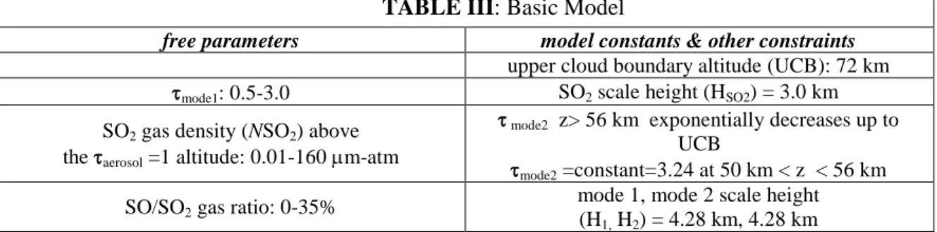
The basic model parameters are summarized in Table III. The SO2 gas density, mode 1 aerosol opacity above the upper cloud boundary (UCB) and the SO/SO2 gas density ratio are free parameters in our model that can be adjusted to match the overall continuum shape of the HST/STIS spectra and the observed gas absorption signatures due to SO2 and SO, which are the dominant absorbers at 200-300 nm. It is important to note that the current RT model assumes that the UCB should be equivalent to the cloud height inferred from 1.4-1.6 µm CO2 absorption signature (Ignatiev et al. 2009); it also assumes that mode 2 particles are only present at altitudes below the UCB. Thus, the UCB defines the upper boundary of the mode 2 particles. Additionally, the current version of the model assumes the scale heights of the mode 1 and mode 2 particles are the same. Notably, this may not be the best representation of the mode 2 particle behavior, as
analysis of the SPICAV-IR occultation observations taken throughout the 8 year period of the Venus Express mission (Wilquet et al. 2009, Wilquet et al. 2012) indicates the larger mode 2 particles may in fact be found at altitudes greater than the previously inferred ~ 70 km cloud top altitude (Esposito et al. 1983) Nevertheless, our current RT model provides the most basic representation of mode 2 particle behavior that is roughly consistent with previous observations and the current analyses of the available SPICAV and VIRTIS nadir observations and is suitable for a first order analysis of the impact of the particles on simulated spectral signatures. In particular, previous observations have shown that in the ±40° latitude region the cloud height relative to CO2 vertical distribution is fairly stable (Ignatiev et al. 2009). Therefore, since all the HST observations are obtained within ±40° latitude, we adopt a single value, 72 km, for the UCB height when fitting all of the HST/STIS spectra. This value is consistent with the average cloud height inferred from SPICAV-IR (1.4-1.6 µm) observations obtained between December 2010, and January 2011 (i.e, VEx orbits 1700 and 1750), see Table II. Lastly, in order to accommodate any residual broadband scattering/absorption in the observations that is not straightforwardly replicated by our base model, we include a brightness scaling factor in our model. This term is equivalent to the factor by which the modeled radiance must be multiplied to match the observed albedo level at 245 nm (where all gas absorption, including that by SO, SO2 and even O3, should be negligible). Notably, because it is the scattering behavior that determines the spectral shape at 245 nm, the inclusion of the brightness factor term by definition implies that our fit of the mode 1 particle opacity is only an estimation and should not be considered to be absolute.
Preliminary analysis of the entire 200-300 nm spectra confirms that the longer wavelength data senses a lower altitude region than that sensed at wavelengths shortward of 260 nm (see Fig. 1). Thus, this paper focuses on replicating the spectral signature observed between 210-260 nm because i) this captures the region where the SO absorption cross-section has been measured in the laboratory, thus is the key region for determining the SO/SO2 gas ratios; and ii) at these short wavelengths the observed albedo is not expected to be significantly impacted by the spectral shape of the unknown UV absorber. I.e., its absorption may impact the observation, but its absorption shape is not expected to change slope rapidly with wavelength in the 210-260 nm region.
Consequently, absorption due to the unknown UV absorber is not included in our simulations.
Based on the parameters described above and the other model characteristics summarized in Table III we complete a least squares fitting of the data in a two part process, first determining the likely mode 1 opacity (τ) above the cloud tops, in conjunction with the likely SO2 gas column density (based on the integration of the SO2 gas density from the top of the atmosphere (TOA) to the altitude level where optical depth unity is achieved in the total aerosol opacity); then refining our constraint of the SO/SO2 ratio and corresponding SO gas density per latitude and time of day, by completing a second least-squares fit of the data allowing the SO/SO2 gas density ratio to be a free parameter in the atmospheric model, ranging from 0-35%. The least-squares fit is estimated relative to the expected error in each of the observed spectra, where the data error is defined based on Poisson statistics and includes the errors introduced by the sky background and the grating scattered light, as discussed in Section 3.
TABLE III: Basic Model
free parameters model constants & other constraints
upper cloud boundary altitude (UCB): 72 km τmode1: 0.5-3.0 SO2 scale height (HSO2) = 3.0 km
SO2 gas density (NSO2) above
the τaerosol =1 altitude: 0.01-160 µm-atm
τ mode2 z> 56 km exponentially decreases up to
UCB
τmode2 =constant=3.24 at 50 km < z < 56 km
SO/SO2 gas ratio: 0-35%
mode 1, mode 2 scale height
(H1, H2) = 4.28 km, 4.28 km
We present in detail the SO2 and SO gas column densities and volume mixing ratios (i.e., relative to the total volume of gas, assuming a CO2 gas abundance of 0.965) inferred from each spatial bin as a function of latitude and time of day in Section 5.
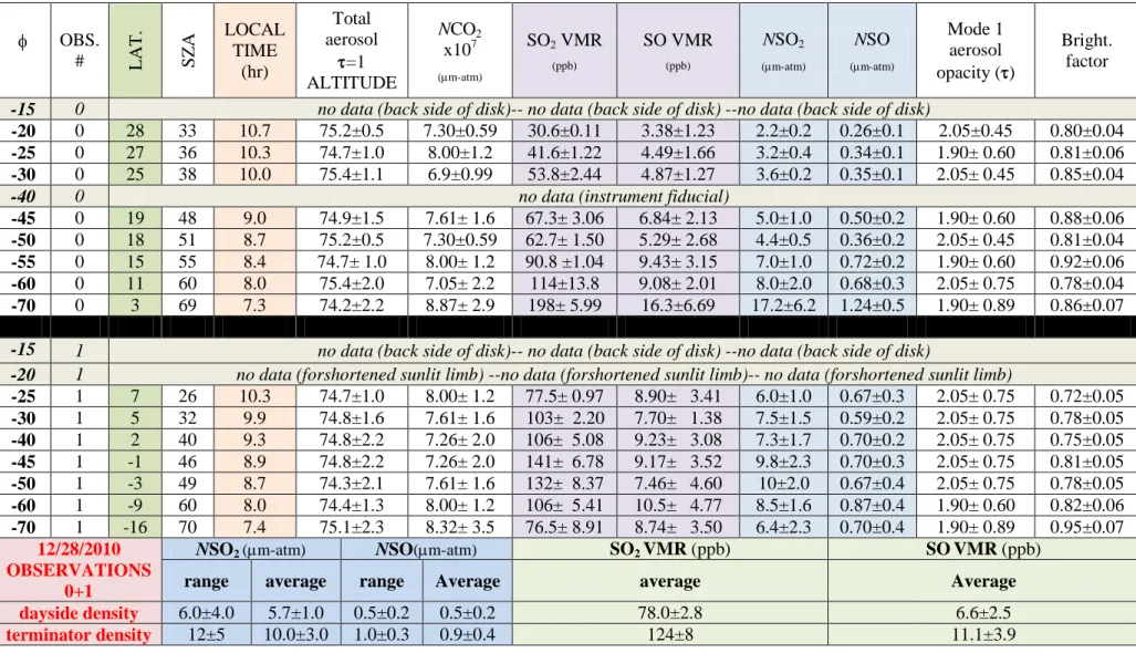
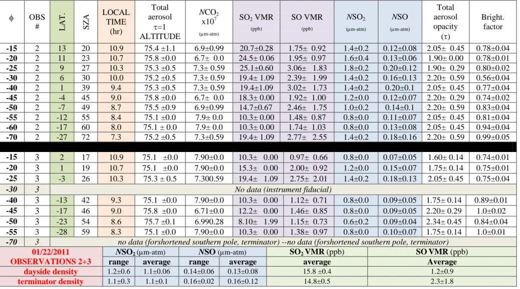
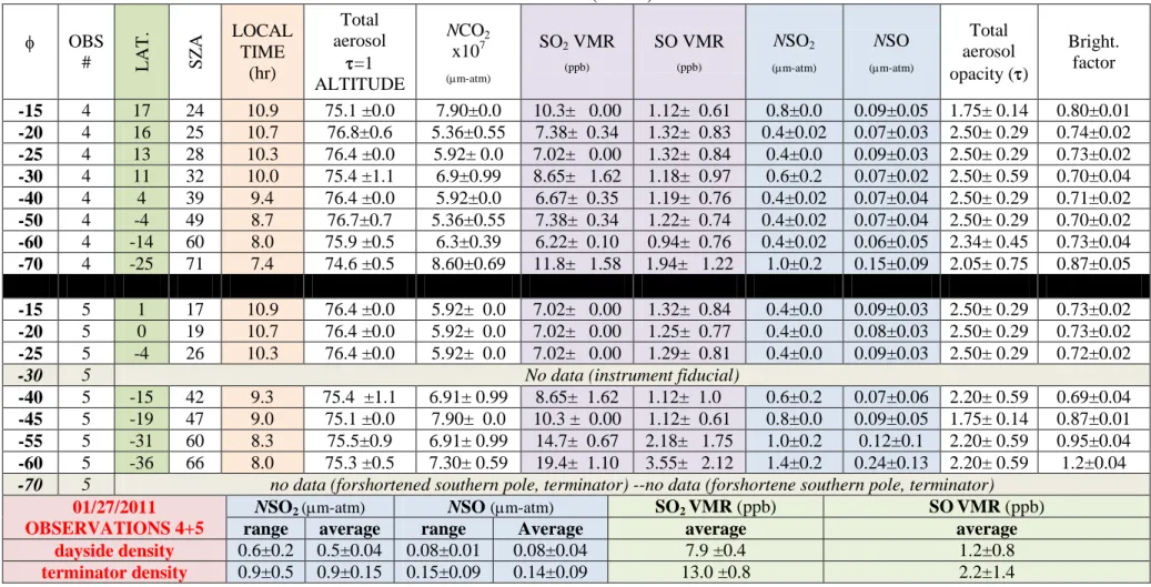
5. Gas Density Results: Inferred Spatial and Temporal Variability of SO and SO2 The SO2 and SO gas column densities and mode 1 aerosol optical depths above the UCB inferred from the least-squares fitting of the data assuming UCB=72 km are summarized in Table IV. For all of the observations the observed spectral signatures are best fit by the model spectra for which the mode 1 optical depth encountered above the UCB at 245 nm is in the range of ~1.0-2.8. Of course, the total optical depth value at 245
nm varies with altitude and is a function of all the aerosol components. Since the entire dataset is best fit when the mode 1 optical depth encountered above the UCB at 245 nm is ≥ 1, the implication is that the total 245 nm optical depth unity altitude always occurs at an altitude greater than the UCB. In particular, with the UCB height set at 72 km, for the fit range of mode 1 aerosol opacities, optical depth unity is always obtained within the 74.8±2.5 km altitude range depending on the latitude and local time of the observation. For all observations at high solar zenith angle (i.e. SZA ≥ 60°) aerosol optical depth unity occurs at an altitude of 75±2 km. Additionally, based on the aerosol profiles assumed in our model (see Section 4), above the UCB the total aerosol opacity is dependent solely on the opacity of the mode 1 particles and CO2 Rayleigh scattering.
Based on the results presented in Table IV we describe trends in the observed SO2 and SO gas distributions as well as the brightness factor as function of latitude and time of day. We discuss these trends based on both the best-fit column densities and the inferred SO2 and SO volume mixing ratios (VMR) where the VMRs are derived using the VIRA (International Venus Reference Atmosphere) CO2 column density (Seiff et al 1985, von Zahn and Moroz 1985) above the inferred total aerosol τ=1 altitude, and assuming 0.965 CO2 abundance. We also compare the HST observations to SPICAV-UV nadir observations obtained throughout the lifetime of the Venus Express mission.
In general, for the 2010 observations the dayside (SZA < 60°) SO2 column densities were in the range of 2-10 µm-atm, while for the 2011 observations the dayside SO2 column densities were in the range of 0.4-1.8 µm-atm. The corresponding average SO2 dayside VMR on December 28, 2010, is ~5 and 10 times larger than that inferred from the January 22, 2011, and January 27, 2011 observations, respectively. The dayside SO column densities on December 28, 2010, were in the range of 0.1-0.11 µm-atm thus 3.5-6x larger than the 0.08-0.20 µm-atm and 0.07-0.09 µm-atm ranges observed in 2011 on January 22 and January 27, respectively. More detailed analyses are provided below. 5.1 Spatial trends in the inferred SO2 gas column density on each observation date:
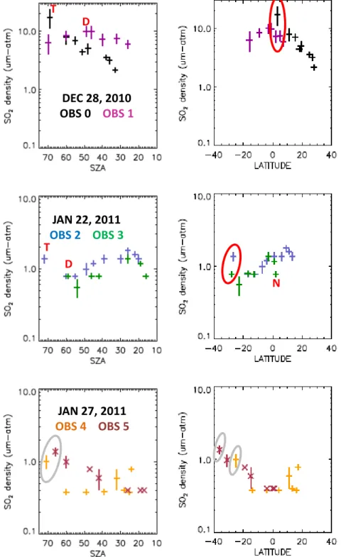
On December 28, 2010, SO2 gas column densities in the range of 2-17 µm-atm were inferred from observations obtained at SZA of 25-70°. The inferred SO2 gas column densities also suggest a strong latitudinal variation, with the largest SO2 gas column
densities found at the equator, at a SZA ~70° (Fig. 7). Notably, the gas densities detected at the equator near the terminator (i.e., at SZA ~70°) are ~ 2x higher than detected at the equator at a smaller SZA, implying that the SO2 gas density is also enhanced on the morning terminator. At the same time, the SO2 gas column density detected at the equator at SZA~70° is almost 3 times larger than that observed near 16S latitude at the same SZA, suggesting the level of enhancement near the terminator may also be latitudinally dependent.
Observations obtained on January 22, 2011 show trends similar to that observed on December 28, 2010 though the SO2 gas density range is an order of magnitude lower extending from 0.6-1.8 µm-atm (Fig. 7). As seen on December 28, 2010, the inferred SO2 gas densities show strong latitudinal variation, with the peak SO2 gas density observed near equator. Likewise, the SO2 gas density observed at 27S near the terminator (SZA~70°) is ~2x higher than observed at similar latitudes at SZA < 60°, suggesting that the SO2 gas density at the morning terminator is enhanced relative to the average dayside SO2 gas density. Additionally, on this date detections of the SO2 gas density near the equator just one hour prior to local noon (i.e., at φ ~ -15°) were made. The retrieved SO2 gas density was a ~ factor of 2 lower than the values obtained ±10° from the equator at SZAs ranging from 20° to 50°, i.e. between a local time of 8:40-10:40 a.m.
As discussed above, the observations obtained on January 27, 2011 were obtained with the same observing geometry as utilized on January 22, 2011. The range of SO2 gas column densities detected on January 27, 2011, is similar to that detected 5 days prior, 0.4-1.4 µm-atm; however, on this date the maximum gas density is observed near 40S latitude rather than at the equator [Fig. 7]. In spite of the change in the direction of the latitudinal variance between January 22 and January 27, the largest SO2 gas column densities again were observed near the terminator. In fact, for OBS4 there appears to be no other sensitivity to SZA above SZA =40° (which corresponds to detections made between 5N to 25S) except for the possibility of an enhancement near the morning terminator at SZA=70° between 25S and 36S latitude. However, comparison of the gas densities detected during OBS4 and OBS5 at comparable latitudes at both high and low SZAs does not show strong evidence of enhancement in the observed gas density detected at high SZA relative to that the gas density detected at SZA <60°. This suggests
that the increased gas density evident near the terminator in both OBS4 and OBS5 is driven entirely by the mechanism supporting the observed latitudinal gas density gradient.
5.2 Trends in the inferred SO gas column density per observation date:
The observed SO gas column densities display behavior similar to the observed SO2 gas column densities: the largest values are observed at the terminator on all three days [Fig. 9], near the equator on December 28 and January 22 [Fig. 8], and at southerly mid-latitudes on January 27. Additionally, the sample correlation coefficient between the SO2 and SO gas column densities (noted as Nso2 and Nso, respectively) across all three
observing dates is 0.97, ignoring uncertainties. Based on a linear regression weighted by the uncertainties on the SO gas column densities but ignoring the uncertainties on the SO2 gas column densities, Nso = (0.08±0.02) * Nso2 + (0.04±0.02). Within the uncertainties
on the retrievals, the inferred SO gas column densities are basically invariant between ±20°. On December 28, 2010 the inferred SO gas density range is slightly lower in the 25N-40N latitude range than in the ±20° equatorial band; while on Jan 27, the inferred SO gas density range is slightly higher in the 20S-40S latitude range than in the ±20° equatorial band. This would seem to imply that variability in the SO gas density is primarily latitudinally driven, and that the gradient in the latitude dependence shows opposing trends in the northern and southern hemispheres. However, it is more likely that the difference in the northern and southern latitude gradients is a function of temporal variation (as a reversal in the SO2 latitude gradient between these dates is also evident), rather than a standing opposing trend in the latitude gradient of the SO gas density between hemispheres (see discussion below). Repeated acquisition of spatially resolved observations that can uniquely measure both the SO2 and SO gas densities would help to clarify this point.
5.3 Comparisons among observation dates:
On all three dates the SO2 gas density detected in the equatorial region between ± 8o latitude was strongly overlapping, thus implying limited sensitivity in the equatorial
SO2 gas density to SZA, for SZA <60°; and on January 27, the latitudinal extent over which the observed equatorial gas density was strongly overlapping was broader corresponding to ± 15° latitude [Fig. 7]. The only exception to the inferred equatorial insensitivity to SZA, for SZA <60° is the factor of 2 difference between the SO2 gas density observed at ~2N, at SZA = 17° vs. that observed between ±10° at SZAs of 20-50° on January 22, 2011. Comparison of the data acquired at a single latitude at both SZA ≥ 65° and SZA < 60° indicates that on both December 28, 2010 and January 22, 2011 the SO2 gas column density near the terminator is a factor of 1.8 to 2.4 larger than that observed at a smaller SZA. On January 27, 2011 comparison of the gas density retrievals made at near equivalent latitude but varying SZA, indicates that the observed gas densities are equivalent within the uncertainty of the fits (see Table IV). This behavior is different from that observed on the other two dates. Thus, as pointed out above, though the gas density observed at 36S at SZA=66° is 1.4x greater than that observed at 31S at SZA=60°, this increase is likely to be either purely latitudinally driven or just a localized enhancement, but it is not consistent with changes driven by the increased SZA [Fig. 7].
As discussed above, the SO2 gas column density inferred from each observation is strongly latitudinally dependent; however, the latitudinal gradient changes sign. Because the January 22, 2011, and January 27, 2011, observations have the same observing geometry and are separated by one cloud top rotation period, the reversal of the latitudinal gradient from that observed on the other two dates is especially significant, suggesting that something other than (or in competition with) a stable pattern in time of day and latitude impacts the observed SO2 gas densities. Looking more closely at the inferred atmospheric properties, the SO2 gas column densities observed between ± 10o latitude on January 27, 2011, are 2-3 times smaller than were observed in that region on January 22, 2011, and the brightness factors fit to the spectra obtained at these latitudes on January 27 are in the range of 0.7-0.73, also smaller than the 0.74-0.83 values inferred from the January 22 spectra obtained within this same latitudinal range. On the other hand, while the near-terminator (SZA ≥ 60°) SO2 gas densities observed in January 2011 were 10-20x lower than the near-terminator values detected on December 28, 2010, the values detected on January 22 and January 27, 2011 were similar corresponding to 0.8-1.4 and 0.4-0.8-1.4 µm-atm, respectively.
The decrease in the equatorial SO2, SO gas density and dayside albedo brightness inferred from the comparison of the December 2010 and January 2011 HST observations may be indication of a number of physical scenarios. E.g., the darkening observed in the 2011 observations may be an indication of the transit of the well-known Y-feature in and out of the slit between late December 2010 and late January 2011, which in itself is an indicator of variance in the density of the unknown UV absorber at these latitudes, due to zonal winds(=advection). However, this is not likely. For one, if the decreased albedo were due to increased presence of the unknown UV absorber, the implication would be that the SO2 gas was decreasing as the unknown UV absorber was increasing which is opposite to previously observed trends (Esposito, 1980; Esposito and Travis, 1982). Additionally, although the VMC imaging is limited to the southern low latitude regions, and our ability to readily identify the contrast in the images is significantly compromised at the latitudes observed closest to the edge of the Venus’ observable disk (see Fig. 5), based on the available imaging there is no evidence of the presence of the Y-feature in the regions coincidently observed by HST and VMC. And lastly, while it is possible the Y-feature was present at low northern latitudes outside of the field of view of VMC, this would require that the narrowest region of the feature intersected the HST slit, since the feature is known to be symmetrical and is expected to extend ±20° of the equator in most cases (Rossow et al. 1980)
A far more plausible interpretation of the coincident decrease in the SO2 gas density and the albedo brightness in January 2011 is that density of the (UV bright) sub-micron haze particles in January 2011 was lower than that present at the cloud tops in December 2010 due to a decrease in upwelling of fresh aerosols or some other dynamically driven change in the chemical processing/formation of the aerosols. A decrease in the mass density of the sub-micron haze particles within the observed time period is consistent with the expected correlation (and co-location) of sulfur-bearing aerosols and the density of the SO2 gas. Additionally, a decrease in the key absorbers (such as micron sized aerosols and other gases) responsible for the infamous dark markings in Venus’ cloud tops should result in cloud top brightness at UV wavelengths that is fairly uniform. Interestingly, the cloud region coincidently observed by HST and VMC shows limited contrast, the general the lack of strong contrast features may be
partly due to the viewing angle. However, inspection of the afternoon quadrant of the projected December 27, 2010 VMC images shows distinct patterns in the cloud contrast at latitudes closest to the edge of the VMC field of view—so that we can confidently say that if there had been significant contrast in the low-latitude morning quadrant cloud top region due to the presence of dark absorption patches it would have been observable [Fig. 10]. The observation of uniformly bright clouds, free of dark absorption patches is consistent with an atmosphere in which vertical mixing and a cut-off of the supply of UV absorbers (including but not limited to SO2 gas) from below the cloud deck has been depressed due to the cooling of the atmosphere (see Titov et al. 2008).
Additionally, while the overall contrast of the 0.36 µm January 22 and January 27, 2011 VMC images was uniform, comparison of the calibrated flux intensity of the cloud tops directly beneath the HST/STIS slit field of view indicates that the 0.36 µm brightness of the clouds northward of 35S was 15% darker on January 27 than on January 22 [Fig. 11]. The gradient of the cloud brightness was also observed to change from increasing towards the equator at all latitudes, to becoming near constant northward of 20S latitude between the two dates. At the same time, the SO2 gas density decrease observed between those two dates was most prominently evident northward of 15S— leading to a change in the gradient of the SO2 latitudinal variation. Therefore, the latitude where the most significant change in the cloud brightness was observed coincides with the latitudes where the most significant change in the SO2 gas density was observed.
5.4 Comparisons to SPICAV-UV observations:
Due to thermal constraints, SPICAV-UV nadir observations could not be included in the original VEx-VCO coordination plan; therefore, no SPICAV-UV nadir observations were taken on the same date as the HST observations. However, SPICAV-UV nadir observations were obtained within 1-2 days of the December 2010, HST observations, and again in March 2011, ~ 1 month subsequent to late January 2011 HST observations. Comparison of the SO2 column densities and overall cloud top brightness levels inferred from the HST and SPICAV data obtained during these time periods indicates that the overall atmospheric variability inferred from the two observation platforms is the same. For example, the average December 2010 SO2 column density
retrieved by SPICAV was ~ 17±4 atm; for March 2011 the value was ~ 0.7±-0.4 µm-atm. In both cases the order of magnitude of the SPICAV-nadir SO2 gas density retrievals was comparable to 2-12 µm and 0.4-1.9 µm values observed by HST in late December 2010 and late January 2011, respectively. Notably the December 2010 SPICAV values were slightly greater than the December 2010 HST retrievals, but this is likely because those observations were obtained at low-latitudes on the afternoon rather than on the morning quadrant. Additionally, both the HST and the nadir SPICAV-UV datasets indicate a decrease in the ~ 0.24 µm brightness of Venus’ low-latitude dayside (i.e. for SZA < 60°) cloud tops between Dec 2010 and March 2011 [Fig. 12]. Additionally, the acquired low-latitude (< 40° latitude) dayside HST observations capture the high and low range of the latitude SO2 gas column densities observed by SPICAV-UV at low-latitudes throughout the entirety of 2011. In fact, the average dayside VMR values derived from the HST observations was in the range of 43± 37 ppb between December 2010 and February 2011, and is identical to the average VMR derived from all the SPICAV observations obtained during 2011 [Fig. 2].
Because of the lower spectral resolution of the SPICAV-UV nadir observations the SO gas column density was not directly retrieved from the available SPICAV-UV observations. Therefore, we do not make a one to one comparison of the HST and SPICAV SO gas density retrievals. Instead, we point out that while Marcq et al (2011) simply assumed the SO gas column density was consistently equivalent to 10% of the retrieved SO2 gas column density, the HST retrieved SO/SO2 ratio ranged ~ 7-18%. These results imply that the order of magnitude of the SPICAV derived SO column densities are reasonable. However, the results also emphasize that in the absence of adequate spectral resolution the latitudinal and local time variation of the SO/SO2 ratio, which may be indicative of changes in the vertical mixing of the atmosphere with time and latitude, cannot be tracked or measured.
Both the larger SPICAV-UV dataset and our small sampling of HST observations indicate that instabilities in the SO2 latitude gradient can be observed [Fig. 13]. The long-term average behavior recorded in the SPICAV-UV nadir observations indicates a decrease in the SO2 gas column density with increasing latitude is the “normal state” of the latitudinal variation, but the reversed SO2 latitude gradient trend is evident when the
lowest equatorial SO2 gas column density is detected (Marcq et al. 2013). Surprisingly, similar to the trends seen in the long-term SPICAV-UV data, our analysis indicates that on January 27, 2011 when the lowest equatorial SO2 gas column density was detected the latitudinal gradient is reversed from the “normal” gradient that increases with decreasing latitude to a gradient that increases as the latitude increases. I.e., on January 27, 2011 the SO2 gas column densities detected by HST within 10° of the equator were equal to 0.4±0.2 µm-atm, which is ~2.5-25x lower than the 1.0±0.2 and 10.0±2.0 µm-atm values observed by HST at equivalent latitudes on January 22, 2011 and December 28, 2010, respectively, at SZAs < 60°.
Interestingly, Marcq et al. (2013) suggests that the gradient of the SO2 latitudinal variation at low latitudes is dependent on the supply of SO2 from below the cloud deck at low latitude. In particular, the Marcq et al. (2013) model specifically proposes that when the vertical mixing rates in the atmosphere are suppressed and remain suppressed for a 4-5 day time period the latitudinal gradient will reverse so that SO2 increases away from the equator; however, the gas density at latitudes outside of the ascending node of the Hadley cell will remain fairly stable over the 4-5 day period, since the photolysis rates at these higher latitudes are also lower. Thus, the observance of low gas densities at the cloud tops in January 2011 by HST, and the corresponding change in sign of the latitudinal gradient in the HST observations from January 22, 2011, to January 27, 2011 at low latitudes, are consistent with the predictions of the Marcq et al. (2013) model.
Additionally, although there was a 2.5x decrease in the SO2 gas density retrieved from the equatorial January 22 and January 27, 2011 observations, the SO2 gas density retrievals obtained between 25-36S latitude in the near-terminator (SZA ≥ 60°) region are equivalent. At a minimum, this implies that whatever the process is that led to the change in the sign of the latitudinal SO2 gradient between the two dates, its impact is most strongly evidenced at low SZA where the impact of photochemical processing is also greatest. Notably, the basic tenet of the Marcq et al. model is that the gas density at high latitude remains stable because of limited photochemical processing in the higher latitude regions. Since this argument also holds for high SZA observations, the observed stability in the near-terminator SO2 gas density retrievals obtained on January 22 and January 27, 2011 is also consistent with the basic tenets of the Marcq et al. model.
If we assume that the observed 0.36 µm cloud top brightness maps to changes in the SO2 and H2SO4 aerosol abundance then the fact that the observed VMC cloud brightness is invariant poleward of 35S latitude on January, 22 and January 27, 2011 while clear differences in the brightness gradient are evident north of 20S latitude is also an indication that the latitudinal variability in the cloud top brightness is directly linked to changes in the upward pumping of both the SO2 gas and other collocated aerosols near the equator, with limited change in the downward flux and photochemical processing of the gas and aerosols at higher latitudes; as also predicted by the Marcq et al. (2013) model.
As discussed above, both the HST and SPICAV-UV nadir observations show that the spectral brightness near 0.24 µm became darker in the time period from late December 2010 to late January 2011; additionally, the 0.24 µm planet brightness was observed by SPICAV to darken over the lifetime of the VEx mission between 2007 and 2011 [Fig. 12]. The darkening observed by HST at 0.245±0.004 µm in spite of the lack of
observable dark patches at 0.36 µm highlights the fact that the 0.245±0.004 µm albedo levels track the haze brightness, and is indicative of the haze properties. In particular, the higher the density of the sub-micron particles the brighter the haze, and conversely the lower the density of the sub-micron particles the more transparent the haze, leading to overall darkening at the cloud tops. Thus, the darkening of the 0.245±0.004 µm abledo levels observed by HST suggests that the sub-micron particle density decreased (either due to a lower influx or due to the coalescence of the particles into larger particles) in the time period from late December 2010 to late January 2011. The fact that SPICAV also observed an overall decline in the 0.24 µm brightness of the planet may also suggest that there was an overall decrease in the sub-micron density over the lifetime of the VEx mission between 2007 and 2011.
6. Gas Density Behavior Inferred from Contemporaneous Gas Density Measurements
6.1 Insights from the coordinated VEx/SOIR +HST/STIS UV observations:
As outlined in Section 2, the HST/STIS observations were coordinated with planned VEx/SOIR observations obtained on December 28, 2010, on the morning
terminator at 31S latitude. The goal of the coordinated HST/STIS+VEx/SOIR observations was to obtain data on SO2 and SO, near the upper cloud top where photolysis is one of the primary drivers of the sulfur chemistry cycle. SOIR’s solar occultation observations can provide the SO2 abundance profile along the terminator at 65-100 km with vertical resolution ranges that vary from 0.2-0.7 km at high northern latitudes, to 2.0-7.0 km in the Southern hemisphere (Mahieux et al 2010). On December 28, 2010, the SOIR vertical resolution was ~ 7 km. On this date, SOIR was only able to positively detect SO2 gas (i.e. set more than an upper limit to its number density) at the terminator at altitudes of 77±3.5 km & 78±3.5 km (6.64-5.39 mbar) above the surface; the retrieved SO2 number density was ~5.3±0.2 x1010 cm-3 at each of these altitudes.
Notably, both the SO2 and CO2 absorption signatures are recorded in the SOIR observations, allowing for the retrieval of the vertical density profiles of both gases, as well as the precise definition of the SO2/CO2 mixing ratio at each altitude where the SO2 gas was positively detected, and the corresponding SO2 VMR (assuming CO2 abundance of 0.965). On December 28, 2010, SOIR retrieved the CO2 vertical number density profile at high precision in the 90-113 km altitude range, below this altitude the CO2 number density values are extrapolated based on the behavior observed in the 90-113 km region and a climatological CO2 profile for lower altitudes (Mahieux et al. 2014a). The extrapolated CO2 number density values are equal to 2.1x1017cm-3 and 1.8x1017 cm-3 at 77±3.5 km and 78±3.5 km, respectively; thus, implying that the corresponding SO2 abundance (VMR) was equal to 290 and 240 ppb in the two respective altitude bins. Notably, the average CO2 number density inferred from SOIR between 74 and 81 km was ~ 1.9x1017 cm-3, while the value derived from VIRA1 is equal to ~2.6x1017 cm-3. In fact, we find that the CO2 number densities derived from the SOIR observations on December 28, 2010, are consistently ~1.37±0.03x smaller than the values cataloged in VIRA at each altitude in the 74-81 km range.
In order to remove any confusion regarding the consistency of the HST and SOIR retrievals we first isolate the average SO2 number density expected in the 74-81 km range from the HST data analysis, and then utilize the same value for the average CO2 number density expected between 74-81 km as inferred from the SOIR observations to derive the SO2/CO2 mixing ratios. In particular, in our model, in order to define specific SO2
column density values at the altitude where optical depth unity is obtained in the aerosol profile the SO2 number density vertical profile is defined as a function of the SO2/CO2 mixing ratio, assuming that both the bulk CO2 atmosphere and SO2/CO2 mixing ratios are exponentially decreasing between 60-100 km. We utilize the SO2 number density profile inferred from the coincident HST observations obtained near the terminator (SZA =70°) at 16S latitude for the comparison to the SOIR observations, since this gas density retrieval was obtained within ~ 15° of the SOIR impact point at 31S latitude, and given the slow variation of the spectral signatures with latitude it is likely to be representative of the gas density located at 16±3S. In this case we find that the average number density observed at 16±3S latitude near the terminator would have been equal to 5.4 x10¹⁰ between 74-81 km; thus, coinciding with the values retrieved from the SOIR observations (Fig. 14) and implying that near identical SO2/CO2 mixing ratios will be retrieved, if identical CO2 profiles are utilized.
Although coincident HST and SOIR observations were obtained only on December 28, 2010, the SO2 number densities and SO2/CO2 ratios inferred from the remaining HST observations in the 74-81 km range can be compared to the coincident 2010 SOIR observations (see Fig. 14) as well as the average behavior observed throughout the lifetime of the mission (see Table V). The temporal variation in the HST-inferred near-terminator (SZA =70°) SO2 number density maps directly to the near-terminator SO2 column density variation discussed in Section 5; thus, the average 74-81 km SO2 number density values inferred from the HST observations are respectively a factor of 5 and 10 lower on January 22 and 27, 2011 than observed by SOIR and HST on December 28, 2010 (Fig. 14). The respective SO2/CO2 ratios for these dates are 280, 52 and 25 ppb if the CO2 number density value inferred from the SOIR observations obtained at 74-81 km on December 28, 2010 is utilized, implying SO2 VMRs of 290, 54 and 26 ppb on these dates (note: the mixing ratio values would be a factor of 1.4 smaller if the VIRA CO2 profiles are assumed). The inferred December 28, 2010 SO2 mixing ratio corresponds to the highest values derived from the low-latitude (i.e. ≤ 40° from the equator) 2006-2013 SOIR observations obtained between 75-80 km (Mahieux et al. 2014b), while the values inferred from the HST observations of Venus’ morning
terminator in late January 2011 are consistent with the lowest low-latitude SO2 VMR values retrieved by SOIR throughout the VEx mission (see Table V).
6.2 Insights from the coordinated HST/STIS UV + sub-mm JCMT observations:
As an additional complement to the coordinated HST and VEx observations, ground-based 346.65217 and 346.52848 GHz observations that are sensitive to the respective SO2 and SO gas abundances in the 70-100 km region of Venus’ atmosphere were obtained between December 28, 2010, and January 30, 2011, using the James Clerk Maxwell Telescope (JCMT) on the Mauna Kea summit in Hawaii (see Table II). On these dates Venus was observed at phase angles of 97-78° (phase 0.44-0.60). The JCMT observations integrate over a 14″ diameter beam. Thus, on each date the JCMT beam was placed at 2 positions offset from the center of Venus’ 28-20″ such that one beam isolated and observed only the dayside morning quadrant (local Venus time ~06:00-12:00), and the other beam isolated and observed only the nightside quadrant (local Venus time ~00:00-06:00). We focus only on the JCMT observations obtained on the morning quadrant, since the 0.2-0.3 µm HST data is only sensitive to the dayside solar reflected signature and on these dates only the dayside morning quadrant was observable from the Earth (see Fig. 4).
To properly interpret the significance of the coincident JCMT and HST retrievals it is important that the observing and analysis parameters of the JCMT data are well understood. For one, since the JCMT observations are beam-integrated they provide a measure of the average dayside morning quadrant gas absorption signature for each date of observation. Additionally, because of the orientation of the JCMT beam, the terminator is located along the edge of the arc of the observing beam; thus, the contribution that this foreshortened region makes to the observed SO2 and SO gas absorption signatures is negligible. Consequently, it is best to compare the JCMT results to the average dayside behavior inferred from the spatially resolved HST observations at SZA <60°. We also point out that the gas absorption signatures recorded in the JCMT observations uniquely characterize the average atmospheric pressure at which the gas detections were made. JCMT observations are converted from pressure to altitude coordinates using a temperature profile specified on a 2 km grid from 66 to 120 km,
representative of theaverage of the spatially averaged dayside temperature measured with the JCMT in the period 1999-2002 (see Clancy et al. 2003). Like SO2 abundance, those temperatures are fundamentally measured as a function of pressure, not altitude. The methods used to assign altitude to the pressure and temperature profiles are described in detail in Clancy et al. (2012), but in brief rely on the assumption of hydrostatic equilibrium and the self-calibration of the derived temperature and gas abundance profiles based upon RT modeling of lower atmospheric continuum emission to define a radiative boundary at 65 km.
We also emphasize that the spectral shape observed in the sub-mm is sensitive to both the magnitude and the shape of the assumed vertical VMR profile of SO and SO2 throughout the 70-100 km region. Thus, the sub-mm observations can be used to distinguish a low-order power-law (or slower) increase with increasing altitude in the SO2 and SO mixing ratios from an exponential (or faster) increase within that altitude range (figures 6-8 of Sandor et al. 2010). In general, all previously obtained sub-mm observations of Venus' atmosphere are well fit by a simple 2 layer model, where the abundance (VMR) above a defined cut-off altitude is significantly higher than below that altitude (Sandor et al. 2010, Encrenaz et al. 2014). If the VMR profile below the cut-off altitude decreases exponentially or faster with increasing altitude then the magnitude of the inferred VMR below the cut-off altitude cannot be distinguished from zero. Thus far, all JCMT obtained high S/N sub-mm observations of Venus’ atmosphere indicate that, taking into consideration the quoted altitude uncertainty per observation, the cut-off altitude between the two layers is located somewhere between 85±3 km. Analysis of these previously obtained high S/N observations of Venus’ atmosphere also indicates that the observed SO2 and SO absorption band shape observations are compatible with vertical profiles for the SO2 and SO mixing ratios that are constant or weakly linear above 85±3 km, but are inconsistent with an exponential increase in the abundances at those altitudes. Additionally, below 85±3 km the SO2 and SO VMR profiles must decrease exponentially (or faster) with increasing altitude. Although the S/N of the JCMT observations coincidentally obtained with HST was poor, the shape of the beam-integrated sub-mm gas absorption band detections obtained by JCMT coincidently with the HST/STIS observations is similar to previous JCMT observations. Consequently, the