WINDII, the Wind Imaging Interferometer on the Upper Atmosphere Research Satellite

HAL Id: hal-01628657

https://hal.archives-ouvertes.fr/hal-01628657

Submitted on 3 Feb 2021

HAL is a multi-disciplinary open access

archive for the deposit and dissemination of

sci-entific research documents, whether they are

pub-lished or not. The documents may come from

teaching and research institutions in France or

abroad, or from public or private research centers.

L’archive ouverte pluridisciplinaire HAL, est

destinée au dépôt et à la diffusion de documents

scientifiques de niveau recherche, publiés ou non,

émanant des établissements d’enseignement et de

recherche français ou étrangers, des laboratoires

publics ou privés.

WINDII, the Wind Imaging Interferometer on the

Upper Atmosphere Research Satellite

Gordon G. Shepherd, Gérard Thuillier, W. A. Gault, B. H. Solheim, C.

Hersom, J. M. Alunni, Jean-Francis Brun, S. Brune, P. Charlot, L. L. Cogger,

et al.

To cite this version:

Gordon G. Shepherd, Gérard Thuillier, W. A. Gault, B. H. Solheim, C. Hersom, et al.. WINDII,

the Wind Imaging Interferometer on the Upper Atmosphere Research Satellite. Journal of

Geo-physical Research: Atmospheres, American GeoGeo-physical Union, 1993, 98 (D6), pp.10725-10750.

�10.1029/93JD00227�. �hal-01628657�

JOURNAL OF GEOPHYSICAL RESEARCH, VOL. 98, NO. D6, PAGES 10,725-10,750, JUNE 20, 1993

WINDII,

the Wind Imaging Interferometer on the Upper Atmosphere

Research

Satellite

G. G. SHEPHERD, • G. THUILLIER, 2 W. A. GAULT, • B. H. SOLHEIM, • C. HERSOM, • J. M. ALUNNI, 3 J.-F. BRUN, 2 S. BRUNE, 4 P. CHARLOT, 5 L. L. COGGER, 6 D.-L. DESAULNIERS, 7 W. F. J. EVANS, 8

R. L. GATTINGER, 9 F. GIROD, 5 D. HARVIE, 4 R. H. HUM, •ø D. J. W. KENDALL, lø E. J. LLEWELLYN, •l R. P. LOWE, •2 J. OHRT, 4 F. PASTERNAK, 13 O. PEILLET, TM I. POWELL, 9 Y. ROCHON, •

W. E. WARD, 1 R. H. WIENS, • J. WIMPERIS •5

The WIND imaging interferometer (WINDID was launched on the Upper Atmosphere Research Satellite (UARS) on September 12, 1991. This joint project, sponsored by the Canadian Space Agency and the French Centre National d'Etudes Spatiales, in collaboration with NASA, has the responsi- bility of measuring the global wind pattern at the top of the altitude range covered by UARS. WINDII measures wind, temperature, and emission rate over the altitude range 80 to 300 km by using the visible region airglow emission from these altitudes as a target and employing optical Doppler interferometry to measure the small wavelength shifts of the narrow atomic and molecular airglow emission lines induced by the bulk velocity of the atmosphere carrying the emitting species. The instrument used is an all-glass field-widened achromatically and thermally compensated phase- stepping Michelson interferometer, along with a bare CCD detector that images the airglow limb through the interferometer. A sequence of phase-stepped images is processed to derive the wind velocity for two orthogonal view directions, yielding the vector horizontal wind. The process of data analysis, including the inversion of apparent quantities to vertical profiles, is described.

1. INTRODUCTION

1.1. Basic Instrument Concept

The WIND imaging interferometer (WINDII) takes advan- tage of airglow emission lines photochemically produced from species in the upper mesosphere (OH), the lower

thermosphere

(02, O(•S)), and the middle thermosphere

(O( • S), O( • D), and O + (2P)) for the measurement

of winds

and temperatures in the altitude range 80 to 300 km. In this section we describe how an imaging field-widened Michelson interferometer is employed for this purpose.

When the optical path difference (the travel time delay between the two paths multiplied by the vacuum velocity of light) in a Michelson interferometer is scanned from zero to some final value, the resulting output is the Fourier trans- form (FT) of the spectrum, which can be expressed as

follows:

lInstitute

for Space

and Terrestrial

Sciences,

York University,

Toronto, Ontario, Canada.

2Service D'A•ronomie du Centre National de la Recherche Scientifique, Verri•res-le-Buisson, France.

3Quantel, Les Ulis Orsay, France.

4AIT Corporation,

Ottawa.

5CNES Centre Spatial de Toulouse, Toulouse, France. 6University of Calgary, Calgary, Canada.

7CAL Corporation, Ottawa.

8Trent University, Peterborough, Ontario, Canada. 9National Research Council of Canada, Ottawa.

løSpace

Science

Division,

Canadian

Space

Agency,

Ottawa.

llUniversity of Saskatchewan, Saskatoon, Canada. 12University of Western Ontario, London, Canada. 13MATRA-ESPACE, Toulouse, France.

14BERTIN, Aix les Milles, France. •5 Interoptics, Ottawa.

Copyright 1993 by the American Geophysical Union. Paper number 93JD00227.

0148-0227/93/93 JD-00227505.00

S(A) =

B(rr)e i2• drr

where rr is wavenumber and /x is optical path difference (OPD). In Figure l a the Doppler-broadened (Gaussian) 557.735-nm atomic oxygen line, B(rr) (one of the emissions selected for WINDID, is shown for a temperature of 200 K. The computed FT, S(A), of this spectrum is shown in Figure lb; it is a cosinusoid having a frequency corresponding to the center frequency of the line, modulated by the FT of the Gaussian line shape, which is another Gaussian, as shown. (The frequency here has been adjusted so that one cycle in the figure represents 20,000 actual cycles.) To obtain such an "interferogram" by direct measurement would require col- lecting about 1 million data points, requiring a very complex instrument that would not be practical for our application. However, a very simple configuration is capable of produc- ing the information required. If the path difference is set to some reasonably large value and then is scanned over only

one period

of the cosinus0id

(for which

the optical

term is

one fringe), the Doppler velocity is manifested as a phase shift of this fringe. The modulation depth, which Michelson defined as fringe "visibility," namely, the ratio of amplitude to mean value, is directly related to the temperature. In this simple configuration the interferometer is a solid unit of cemented glasses, that includes a mirror cemented on piezo- electric drivers, so that it can be stepped in small steps over an OPD range of one wavelength.

If we let v be the wind velocity, k the interference order, c the velocity of light, then the phase shift is

rb - 2rrk- (2)

c

For k - 10 5 and v - 10 m s-i, rb = 1.2

ø. This resolution

is

achievable by an instrument having a size compatible with space flight requirements.

10,726 SHEPHERD ET AL,: THE WIND IMAGING INTERFEROMETER (a) Ol 557.7 nm Spectrum at 200 K 1.2 1

0.8

0.6

0'1t

3 5 10

15

20

Optical Path Difference - cm

0.8 (c) OI 557.7 nm Spectrum at 1000 K 1.2 0.2 (d) 1000 K Int•rferogram 2 1.5

• 1

-'

•/

. ø'

I

Fig. 1. (a) The spectral line shape of the atomic oxygen 557.7-nm emission at 200 K and (b) the corresponding Fourier output of a Michelson interferometer (MI) called an interferogram. (c) The 557.7-nm spectral line shape for 1000 K and (d) the corresponding interferogram. For the interferograms, one cycle in the figure represents 20,000 actual cycles.

by the instrument; and Ia is the atmospheric background

light which enters the interferometer through the interfer-

ence filter selecting the atmospheric line to be observed. Since only three parameters (visibility, phase, and mean intensity) can be extracted from an interferogram, Ia needs to be measured by another means, following which it is

subtracted from S(x) to form the background-corrected signal I(x):

Z(x) = S(x) - (5) The requirement of determining the absolute phase (2½rA/A) is avoided by using a relative phase 0 = 2½rA/A - 2½rrn, where rn is an unknown integer and 0 < 2•r. The penalty for

this is that the "zero-wind" phase must be determined later through instrument calibration.

After generating an interferogram by varying x from 0 to/5,

we may calculate

1;•=

I(xi)

dx

Jl=•' 0

f i'•= 2

'n'x

i

2

I(xi)

cos

J2=•' 0

A

fi•= 2•'xi

2

I(xi)

sin dx

J3

= -•- 0

A

When the summation is made over an integral number of fringes, we have

J1 = Io (9)

J2 = UVIo cos 0 (10)

For the determination of the temperature the fringe visi- bility V is related to the temperature T by

V = exp [-QoA2T]

(3)

V is the line visibility as given by (3) where Q0 = 1.82 x

106/(M A0•),

M is the atomic

mass

(gram)

of the species

emitting the line centered at A0, and A 0 is the line wavelength at rest.

In Figure 1 c we show the line shape for the same atomic oxygen 557.735-nm emission shown in la but for a temper- ature of 1000 K. The effect on the interferogram is shown in Figure 1 d, which illustrates through comparison with Figure lb that the temperature can be determined at a fixed path difference, by stepping the OPD over a single fringe.

The equation corresponding to the interferograms of Fig- ure 1 but defined in terms of an instrument that makes small OPD steps of size x from a reference optical path difference A 0 is, where we have changed our variable from •r = 1/A to

A,

S(x) = Io

A0

+

x

1

1 + uv cos 2•- + I• (4)

I0 is the line intensity; A is the Doppler-shifted line wave- length (/am); U is the visibility reduction factor introduced

J3 = UVIo sin • (11) from which I0, V, and 0 may be determined if U is known. The actual procedure used for WINDII atmospheric data

is described in section 3.1. Knowledge of V leads to the

temperature as already described, and 0 is the total phase which includes the intrinsic interferometer phase (0i = 2½rrn), the phase induced by the velocity of the spacecraft (0s), the phase induced by the Earth rotation (0r), and the phase induced by the wind to be measured (0,,); 0i, 0r, and 0s depend on the line of sight position in the instrument field of view and are known either from calibration data or calculated from the spacecraft attitude and velocity. Having 0 from above and knowing 0i, 0r, and 0s, one can then derive 0,, from the measured 0. The wind velocity along the particular line of sight used for the measurement is calcu- lated from

27r u

Ow=•D - (12)

A o c

where D is the interferometer effective optical path differ-

ence given by [Thuillier and Hers•, 1991].

SHEPHERD ET AL.: THE WIND IMAGING INTERFEROMETER 10,727

F ou1 FOU• Degrees

137.4 .145.6 153.8 178.3 186.? •94.9 •83.1 •11.4 •19.G • ... 835.8

Plate 1. WIND imaging interferometer (WINDII) phase image for 738.4 nm obtained from the Argon on-board calibration lamp. Note the color scale which extends from 105 ø to 235 ø . The image is symmetrical about the bottom center of the CCD image, which is the

location of the Michelson interferometer axis. Because of field

widening, the phase variation is only 130 ø, over an off-axis angular change of 10 ø inside the interferometer.

Its value is measured during the instrument characterization

and is available for use.

An example of a phase image for the 738.4-nm line from the on-board Argon spectral lamp (Table 4) is shown in Plate 1, as obtained from a sequence of four images, applying (6)-(11) on a pixel by pixel basis. The phase begins at 235 ø on the interferometer optical axis located at the center bottom of the CCD and falls to about 100 ø at the top, before rising to

160 ø at the corners. This small variation in phase is observed

because the Michelson interferometer is field-widened, oth-

erwise the phase change would be several hundred thousand

degrees.

Array detectors, such as CCDs, provide a capability for quantitative imaging using just a camera lens and a CCD. In principle, a camera can be made into a spectroscopic imager by placing a band-limiting element in front of the camera lens. However, all spectral band-limiting elements introduce a transmittance that is dependent on the off-axis angle.

Interference filters such as employed in WINDII have a

wavelength

of peak

transmittance

given

by •'i = Ap

i2/2n2,

where

Ap is the wavelength

of peak

transmittance

for normal

incidence, Ai is the wavelength of peak transmittance at

angle i, where i is the incident angle of the ray and n is the

effective refractive index of the interference filter. The

transmittance of the band-limiting element thus varies across

the image in a way that depends on the quantities introduced

above and the passband width. The Fabry-Perot etalon presents a more extreme case in which spectral rings are superimposed on the image. Such devices still qualify as imagers, such as the Rees et al. [1984] Doppler imaging interferometer and the Kendall et al. [1985] Oglow camera, but the spatial information is mixed with the spectral infor-

mation, the two being multiplied together. Of course one cannot record two-dimensional spatial information and spec-

tral information on a single two-dimensional detector; a

choice must be made.

With WlNDII the intent is to record full two-dimensional

spatial images characterized by a single OPD value; an

internal mirror movement is used to step the OPD value through four (or eight) positions and record an image at each

position. We have chosen to make the OPD steps sequential

in time in order to achieve full imaging in the sense that a wind value is obtained for every pixel for which sufficient airglow emission exists to make a measurement. In fact, the OPD does vary over the field of view, producing the type of phase variation in the image shown in Plate 1, but because the interferometer is field-widened, the variation is small enough to be readily calibrated. An interference filter is also

required in front of the Michelson to select particular emis-

sion lines. The instrument transmittance for a single emis- sion does vary over the field of view, but again it is a variation that can be readily calibrated. This characteristic can also be exploited: one of the WINDII filters is adjusted so that it transmits OH emission at the bottom of the image

(the lowest

altitude)

and O + emission

at the top. For the O2

emission, which has closely spaced rotational lines, different

lines are imaged at different places on the CCD.

The measured velocity we have described thus far is

simply the component along the line of sight. WINDII employs two view directions, at 45 ø and 138 ø from the

velocity vector on the anti-Sun side of the spacecraft. Images taken simultaneously in both directions are recorded side by side on a single CCD. Pairs taken roughly 7 min apart are combined to give orthogonal wind vectors from the same

volume of atmosphere, on the assumption that the wind does

not change in that time.

1.2. Heritage

In response to the Upper Atmosphere Research Satellite (UARS) mission opportunity announced in 1978 the wind and temperature by remote sensing (WINTERS) instrument proposed by France with G. Thuillier as principal investiga-

tor was one of those selected in 1979. It was based on the

concept of a field-widened Michelson interferometer [Bou- chareine and Connes, 1963] which uses refractive materials in the arms of the interferometer to provide much larger

fringes, at a given path difference, than for an ordinary

Michelson interferometer. Hilliard and Shepherd [ 1966a, b] conceived a simple configuration of this instrument, operat- ing at an essentially fixed path difference, for the measure- ment of atmospheric temperature. This instrument had great

sensitivity for temperature but could not be used for wind

measurements due to its inherent sensitivity to instrument

temperature change. A passive system designed to cancel this undesirable effect was proposed by Thuillier and Shep-

herd [1985] and adopted by the WINTERS instrument and

its ground-based version called MICADO. The approach is

an extension of the method described by Title and Ramsey [1980]. The WINTERS instrument based on the Thuillier and

Shepherd [1985] concept includes optical fibers, photomul- tiplier detectors, and mechanical scanning of the two fields of view as in the high-resolution Doppler imager (HRDI) design. The UARS mission was not approved for implemen- tation until 1984, and by that time there were insufficient resources available in France to build the entire instrument. It was therefore agreed to join forces with Canada, in order to share the cost but also to take advantage of what had already been developed in both countries. Canada had developed, for a Spacelab flight, an instrument called wide angle Michelson Doppler imaging interferometer (WAMDII)

10,728 SHEPHERD ET AL..' THE WIND IMAGING INTERFEROMETER

[Shepherd et al., 1985], which took advantage of recently developed CCD technology as well as new piezoelectrically driven positioners. In France, studies had been carried out for the WINTERS project and construction had begun on the MICADO instrument which was to be operated as a correl- ative measurement experiment during the UARS flight.

The combination of fundamental concepts available from

the WINTERS and WAMDII thus formed the basis of a new

instrument, called WlNDII. The remainder of this paper is concerned with a presentation of the WlNDII instrument.

1.3. Expected Contribution to Upper Atmosphere Research Satellite (UARS) Goals

The UARS mission is dedicated to the measurement of

energy input, abundances of minor species, temperature, and winds in the stratosphere and mesosphere in order to study their mutual relationships and to build and validate atmospheric models. The wind is a key to the understanding of atmospheric behavior because it transports energy and species from one location to another and represents the response of the atmosphere to the net forcing imposed on it. The importance of wind measurement was acknowledged early in the history of the study of the Earth's atmosphere, but actual data for the stratosphere, mesosphere, and lower thermosphere have been slow to appear, owing to the intrinsic difficulty of the measurement. For this reason, indirect means involving the assumption that the winds satisfy some sort of balance condition have typically been used for their determination. The wind field most simply calculated and most often presented is that based on geo- strophic balance and the observed temperature fields [An- drews et al., 1987, pp. 224-225] although other alternatives have been explored (see Randel [1987] or Marks [1989] for a discussion). This indirect method, however, only addresses the large-scale average winds and suffers significant difficul- ties at low latitudes, where the geostrophic balance breaks down, and at high latitudes in the thermosphere where electromagnetic forces start playing a significant role in driving the neutral circulation [Richmond, 1991]. In addition, the assumption that the circulation is constantly in balance has never been directly verified on a global basis and the nature of this balance is one of the topics we hope to address

with WlNDII. Another region of particular interest to WIN-

DII is the extratropical upper mesosphere/lower thermo- sphere where one of the dominant sources of energy is the dissipation of gravity waves and tides. The nature of the dynamics in this region has traditionally been examined using the transformed Eulerian mean equations, the temper- ature fields, and the radiative transfer codes (see, for exam- ple, Solomon et al. [1986] or Shine [1989]). With a suitably averaged data set of horizontal winds from WlNDII, it should be possible to examine these dynamics from a new perspective.

To date, most of the measurements of middle atmospheric winds have been obtained through the use of radiosondes, rockets, and radars. Optical instruments have provided a good deal of information about winds in the thermosphere through measurements from space [Killeen and Roble, 1988] and from the ground (see, for example, Burnside et al. [1981]; Hernandez et al. [1982]; Batten and Rees [1990]; Thuillier et al. [1990]; Wiens et al. [1988]). This technique takes advantage of naturally occurring airglow emissions

above 80 km which contain information about wind and

temperature. This information can be extracted by using interferometers such as those of Fabry-Perot or Michelson. The passive optical method is the most amenable to space- flight.

WlNDII is one of two UARS instruments dedicated to the

measurement of atmospheric dynamics, specifically of global winds. The other instrument, HRDI, has as its primary goal the measurement of winds in the upper troposphere, strato- sphere, and mesosphere using a triple-etalon Fabry-Perot spectrometer that observes the shifts of absorption lines in scattered sunlight. WlNDII is a Michelson interferometer that measures the wavelength shift of emission lines in the Earth's airglow, beginning at 80 km near the mesopause and extending up through the thermosphere, with the primary emphasis being in the range 80 to 110 km. The design of HRDI revolves around the requirement of a single narrow passband, to permit the measurement of an absorption line in the presence of the large scattered white light background. This requirement leads to a small field of view. While it can also measure emission lines in the airglow, the dominant requirement makes it less sensitive than it would otherwise be, and so it will be used for that purpose on a limited basis. The Michelson interferometer and the Fabry-Perot spec- trometer are complementary by their nature, as one works in spectral space and the other in OPD space. WlNDII has a very low tolerance to white light but has extremely high sensitivity; it is designed specifically for the study of weak airglow emissions. Thus the complement of HRDI and WlNDII are well suited for covering the range of altitudes of interest for dynamics measurements to support the UARS mission. The Fabry-Perot instrument is well accepted for the measurement of winds, as demonstrated with the FPI instru- ment on the Dynamics Explorer 2 spacecraft [Killeen et al., 1984; Hays et al., 1984]; long before that, it was used for the spaceborne global measurement of temperature [Thuillier et al., 1980; Blamont and Luton, 1972]. The wide angle Mich- elson is a less mature instrument, although the device had been under development for some time in Canada [Hilliard and Shepherd, 1966a, b; Shepherd et al., 1984, 1985, 1991; Ward, 1988] and in France where the MICADO instrument is now operational in the field [Thuillier and Hers•, 1991; Thuillier et al., 1990]. The UARS mission will provide the first spaceflight opportunity for this technique. The capabil- ity of HRDI and WlNDII to make measurements in an overlapping altitude range permits an important opportunity to compare the results and performance of these two rather different approaches.

In the UARS mission, WlNDII has the responsibility of extending the wind measurements, made at lower altitudes by HRDI, up to 110 km. For this purpose we use Doppler shifts of narrow emission lines emitted by the visual airglow. This restriction can be met by the choice of three prominent

emissions:

atomic

oxygen

O1S at 557.7 nm, at night a thin

layer near 97 km, the 02 atm band emission at 763 nm which

also emits at night in a thin layer near 94 km, and finally OH which emits in a thin layer centered at 85 km. During the daytime the first two emissions are intensified by additional processes, and they are measurable against the background of Rayleigh and baffle scattering. The UARS requirement is for a measurement every minute, so if two different emis- sions are used, a complete measurement for one emission

SHEPHERD ET AL.: THE WIND IMAGING INTERFEROMETER 10,729

The principal objective is to provide global measurements of wind for comparison with current global circulation models (GCMs) and, in so doing, identify those processes responsible for wind forcing at these altitudes. The meso- sphere is an important interface between the stratosphere, largely controlled by radiative processes, and the thermo- sphere which is controlled by a combination of photochem- ical and electromagnetic processes. It is thus influenced by forces from above and below. From above, the energy input

into the aurora and the associated electric fields and currents

drive the ions, which transfer momentum to the neutrals. This influence is well established in the F region where Doppler measurements have been made with the 630.0-nm atomic oxygen emission. What is not known is how low in the atmosphere the effect penetrates. Electrodynamic effects as well as auroral heating appears to launch gravity waves that move equatorward, producing heating effects that have been observed in the 630.0-rim emission at the equator. Some WINDII observing time will be allocated to investi-

gating

these effects,

using

the 630-nm

O(•D) emission

for

neutral

winds and the 732- and 733-nm

O+(2P) lines for ion

winds.

From below, gravity waves produced near the Earth's surface propagate up to the mesopause region, where they

"break" and interact with the mean flow. The influences

from above operate in a frame of reference attached to the Sun, with dynamical perturbations that can be correlated with magnetic disturbances. The intensity of gravity waves propagating from below is determined by the forcing mech- anism at the surface and the filtering due to the wind field in the intervening atmosphere. Variations, associated with these factors, in the observed amplitudes of these waves are expected to be observable and so should appear in the daily wind maps. The appearance of such daily patterns would constitute a major discovery and provide unambiguous evi- dence for coupling from the troposphere to the mesosphere.

On a smaller scale, the identification of the characteristics of individual gravity waves would be of great importance. Observations of the longitudinal, latitudinal, and seasonal variations would be very valuable. Observations of vertical gradients in horizontal wind variances would permit evalu- ation of momentum transfer and gravity wave breaking. Simultaneous measurement of the background winds will allow the breaking process to be investigated. Quite apart from the wind measurements, measurement of temperature and emission rate will be made; these also have gravity wave signatures. Here the capability of measuring rotational and Doppler temperatures will be of great interest. The long integrating paths at the limb will tend to smear out wave structures, but as yet we are unable to say to what extent the short wavelength wave will be observable.

Tides are another influence from below that need to be

investigated [Forbes, 1982a, b]. As with gravity waves, they increase in amplitude with height and are thought to break in the lower thermosphere. While it is not clear that WINDII samples frequently enough over a large enough spatial region to unambiguously resolve the spatial varia- tions of all the tidal modes, it will certainly contribute to investigations of their nature.

Volume emission rates permit the deduction of certain species concentrations, in particular atomic oxygen, al- though other species are of interest as well. This will allow studies of the transport of O, and direct correlations between

species concentrations, and their advection by the observed winds. From such a study, photochemical time scales may be derived and the coupling between the dynamics and the horizontal variations in species concentration investigated.

In addition to the primary mandate of UARS, individual

team members have interests that extend well into the

thermosphere, which is consistent with the UARS objectives that call for a study of coupling between regions. Optical measurements will necessarily detect aurora and give a measure of local energy input, supplemented by the particle environment monitor (PEM) measurements (particularly its X ray imager AXIS which views in the same direction as

WINDII). Optical measurement

of O + gives ion winds,

which in turn allow ion-neutral momentum transfer to be studied. Enhanced winds and convection near auroral forms

are expected, since there is now considerable evidence for upwelling and atomic oxygen depletion near auroral forms. Although a thermospheric phenomenon, such depletions are likely to be one of the sources of variations in atomic oxygen and hence provide a mechanism for coupling between the thermosphere and the mesosphere.

1.4. Characteristics of the WIND Dnaging Interferometer (WINDII) Target Emissions

WINDII fundamentally measures the modulation of two line of sight interferograms for various emission features; from this modulation the apparent Doppler velocity, Doppler temperature, and emission rate are determined. The two data sets may be combined to provide a limited tomographic capability. Combining the emission rates for different spec- tral lines within a single molecular band allows rotational temperatures to be obtained as well [Mende et al.. 1988]. By inverting these data, vertical profiles of these same quanti- ties are derived. However, because of the numerical proce- dures involved and the necessary assumptions for the anal- ysis, the results from these inversions require a knowledge of the emission characteristics. Further quantities, such as the vertical profile of atomic oxygen concentration, may be determined from the volume emission rate profiles [Evans et al., 1988]. From the concentration profile, the temperature profile, and the vertical wind gradient, it is possible to derive diffusivity coefficients. Table I lists both the directly mea- sured and the inferred quantities.

The upper mesosphere/lower thermosphere emissions (the oxygen green line, the oxygen atmospheric band, and the hydroxyl vibration/rotation bands) are essentially confined to narrow layers in the altitude region 85-97 km. Thus the requirement of good definition for the emission height pro- files demands that the pixel bins be selected so that they reflect this narrow height range. However, there are a number of observations [Swenson et al., 1989] which suggest that the emission layer heights are not as constant as is often assumed, so that the limited height range sampled from the

CCD must be selected to reflect these known variations. As

the mesospheric emissions are known to exhibit wave struc- ture, the full detailed analysis of the observations requires the stereoscopic capability afforded by the two WINDII

fields of view.

Quantities that are measured by WINDII are emission rate profiles, wind profiles, and temperature profiles. Although the apparent properties are measured directly, they must be inverted to obtain the actual quantities. In order to properly

10,730 SHEPHERD ET AL.' THE WIND IMAGING INTERFEROMETER

TABLE 1. WIND Imaging Interferometer (WINDII) Measured and Inferred Parameters

Quantity Measured Conventional Method of Measurement

557.7-nm volume emission rate 557.7-nm wind

557.7-nm temperature 630.0-nm volume emission rate 630.0-nm temperature 630.0-nm wind O + emission rate O + wind OH emission rate OH wind OH Doppler temperature OH rotational temperature

02 atmospheric (atm) volume emission rate 02 wind

02 rotational temperature Rayleigh scattering temperature Gravity wave characterization? Diffusivity?

Atomic oxygen concentration?

rocket

GB FP, GB WAMI, rocket,* radar

GB FP, GB WAMI rocket

incoherent scatter, GB FP, GB WAMI

GB WAMI, GB FP, rocket,* radar

GB scanning interferometer

incoherent scatter radar GB FTS

GB FP, GB WAMI, radar, rocket* Lidar, rotational temperature GB FTS, spectral imager

rocket

rocket,* radar, GB WAMI, HRDI

GB spectral imager, rocket lidar, HRDI

GB WAMI, radar, lidar rocket

rocket

GB, ground based; FP, Fabry-Perot; FTS, Fourier transform spectrometer' HRDI, high-resolution

Doppler imager; WAMI, some form of wide angle Michelson interferometer.

*Radar chaff or chemical trails.

?Denotes inferred quantity.

interpret the results it is essential

to have a knowledge

of the

emission processes. For example, it is important to recog-

nize that all of the emissions used here are forbidden: in the

mesosphere

and lower thermosphere

the emitting species

suffer sufficient collisions between excitation and radiation,

so that the emissions are characteristic of species in thermal

equilibrium

with the surrounding

gas (radiative lifetimes are

given in Table 2). In the middle thermosphere,

where colli-

sion times are longer, this is not necessarily true. The various airglow emissions associated with the recombination of atomic oxygen originate from different altitudes in the atmosphere [Llewellyn and McDade, 1984]. Thus measure-

ments of these different features can provide atomic oxygen concentrations at several different altitudes. Height profiles

are possible

through

measurements

of the OH Meinel bands,

the 02 atm (0-1) band,

and the O1S green

line. Character-

istics of the emissions are given in Table 2, which apply to both daytime and nighttime.

There are two regions of excitation for the airglow, with recombination of the atomic oxygen layer causing excitation of the nightglow in the 100-km region and ionic recombina-

tion processes exciting emissions in the 150- to 300-km

region. For example, at levels above 150 km the green line emission is excited by dissociative recombination:

0•- + e-->O(iS) + O.

Photoelectron fluxes from daytime ionization by solar EUV photons and electron fluxes from auroral precipitation en- hance the ion production and excite the green line at

intermediate levels from 100 to 200 km. The same processes

excite

O(•D), the upper state of the red line emission:

0•- + e-->O(iD) + O.

For the thermospheric emissions the quality of the WIN-

DII data are such that it should be possible to extract any

mesospheric

component

(e.g., as in the case

of the O(•S)

green line) and to identify the emission components that are excited in different ways. In particular, the oxygen red line is excited by both dissociative recombination and by photo- electron impact, in a process similar to that in the aurora. The dissociative recombination process can lead to hot atoms, with a large spectral line width, while the electron

impact will give normal line widths. Thus the observations

can be used to identify both the excitation impact cross

section and the atomic oxygen profile. Below 150 km the

O(•D) atoms

are quenched

by molecular

nitrogen

and oxy-

gen to give the oxygen atmospheric band emission, an

Emission

TABLE 2. Emission Characteristics

Lifetime, Wavelength, Height Range,

s nm km O 1S green line 0.8 O 1D red line 110 OH (8-3) band 4.2 ms 02 atm (0-0) band 14 O + line 5 Green continuum Rayleigh scattering Peak Altitude, km 557.7 lower 80-110 upper 150-300 630.0 150-300 730.0 80-110 762.0 80-110 732.0 200-300 500-900 80-120 500-900 80-120 97 200 -250 87 94 -150 90 exponential falloff Half Width, km 15 50 - 100 10 10 -50 20

SHEPHERD ET AL.' THE WIND IMAGING INTERFEROMETER 10,731 emission that is also studied with WINDII. Thus WINDII

has the capability

to make measurements

of the O(1D)

population to lower altitudes than is normally possible.

At lower levels the green line of atomic oxygen is excited by the reassociation of atomic oxygen in the atomic oxygen

layer at 100 km and the subsequent energy transfer [McDade

et al., 1986]:

O+O+ M--> O2'

+ M.

O2

• q- O• O(1S) q- O•.

The hydroxyl emission originates from the recombination of the atomic oxygen layer into ozone and the subsequent reaction with atomic hydrogen to form vibrationally excited hydroxyl, which emits into numerous bands, including the (8-3) band observed by WlNDII [Murtagh et al., 1987]:

O + 02 + M--•O 3 + M 0 3 q- H-• OH* + 02.

The recombination of atomic oxygen into molecular oxygen and the subsequent energy transfer can also lead to the

excited

electronic

state,

O2(1•), which

is the radiating

state

for the 02 atmospheric band emission:

O+O+ M--> O2'

+ M.

02* + 02-• O2(•Z) + 02.

O2(1•) is also

excited

by energy

transfer

from O(1D) in the

day airglow;

the O(1D) is produced

by ozone

photolysis

and

by photodissociation of 02 and of H20 by ultraviolet sun-

light. There is also a daytime contribution to the atmospheric band emission from the resonant scattering of sunlight.

The interpretation and conversion of the measured quan- tities into meaningful geophysical quantities requires the knowledge of both the kinetic temperature and the atmo- spheric density in the emission region. The kinetic temper- ature is measured from the emission itself, but for the density we must use either a model, which is itself uncertain, or the absolute intensity of the Rayleigh scattering.

The high altitude O + emission

at 732.0/733.0

nm is excited

mainly by EUV photoionization (h < 67 nm) during the day

and in twilight, while at night, auroral electron precipitation can excite this species as follows:

O + e --->

O+(2P) + 2e.

O + hv --> O+(2P)

Thus the daytime emission may be used to study the variation in the solar EUV output as well as atomic oxygen concentration [McDade et al., 1991], extending the range of the solar spectrum monitored by UARS into the UV. Ray-

leigh scattering of sunlight by 02 and N2 occurs in the

daytime and creates a continuum background in all channels at low altitudes. The intensity of this scattered light de- creases exponentially with altitude with a scale height of about 7 km. Measurements of the intensity variation with altitude can be used to measure the temperature at lower altitudes, and the absolute values will yield a measurement of atmospheric total density.

The green continuum comes from the recombination of nitric oxide with atomic oxygen [Swenson et al., 1985]:

I Electrical

c

Instrument Sensor Unit (ISO)

Power Interface Circuits (P•C) Instrument Control & Data Handler (ICDH) Electrical Unit (EU)

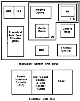
Fig. 2a. Block diagram of the WINDII system. OBA, outer

baffle assembly; IBA, inner baffle assembly; MI, Michelson inter- ferometer; MCC, mirror controller component; ITE, inner thermal enclosure; and OB, optical bench.

NO + O--> NO•.

This emission is weak but contributes a significant signal in the wide band-pass background channels in the altitude region from 80 to 100 km.

During auroral events in the polar regions, energetic particle precipitation enhances most of these emissions and increases the brightness of the green line and red line emissions by manyfold. Thus auroral winds and tempera- tures may also be investigated.

2. DETAILED INSTRUMENT DESCRIPTION

2.1. Overview

The WINDII system consists of a flight segment (the instrument) and a ground segment (remote analysis com-

puter (RAC)). The instrument is comprised of two units: the

electrical unit (EU) and the instrument sensor unit (ISU). The ground segment consists of the RAC hardware, soft- ware, and network connections. A system level block dia- gram of the instrument is shown in Figure 2a and a drawing of the assembled physical system in Figure 2b.

The EU houses the microcomputer controller (instrument

control and data handler (ICDH)), power regulation, condi-

tioning and distribution circuits, interfaces with a UARS remote interface unit (RIU) for telemetry and command, interfaces with the UARS power supply unit (PSU) for quiet,

pulse, and survival power busses, and the calibration laser.

The ISU contains the outer and inner baffle assemblies, the imaging optics, Michelson interferometer, CCD camera,

calibration component, mirror controller, electrical interface

circuits, thermal control heaters, thermistors, thermostats,

blankets and radiator plates, pyrotechnic devices, and inter- faces.

In terms of operations the EU ICDH receives command data from the UARS RIU and executes daily experimental

10,732 SHEPHERD ET AL.' THE WIND IMAGING INTERFEROMETER THERIffAL RAD I A TOR REAR FILTER HICHELSON INTERFEROHETER AND THERHAL ENCLOSURE

CCD CAHERA

INTERFACE IT FIELD TELESCOPE

BAFFLE A$SY ELECTRICAL AND FIBRE OPTICS THERRAL ENCLOSURE POINTS TO UARS (! OF 3) OUTER BAFFLE ELECTRICAL U~lr •

Fig. 2b. WINDII configuration. The two orthogonal input beams enter through the two ports on the lcœt, in the

outer baffle assembly, and cross over before entering the inner baffle assembly and then the split field telescope where the two inputs are combined into a single beam. This beam passes upward through the filter wheel and the rear telescope before entering the Michelson interferometer, in its thermal enclosure. The CCD camera is located immediately behind the Michelson interferometer. Calibration light is introduced at the circular ports on the inner baffle assembly by an optical fiber harness (not shown). The laser is located in the electrical unit, and the light is transported through a fiber optics cable along with the electrical cabling.

programs based on data tables updated by the uplinked commands. Telemetry containing image data and engineer- ing information is formatted by the ICDH and transferred to the RIU for downlink using the 2000 bits/s allocation for WINDII. The experimental parameters for each measure- ment are determined by the flight software resident in the ICDH and are provided to the ISU on a bidirectional 1-MHz

serial data link. This connection also allows the CCD camera

data to be transferred to an image data buffer in RAM within the ICDH memory. A limitation on the amount of image data from a measurement of 20480 bins is based on the constraint of 32 kbytes of image RAM.

The ISU electrical interface circuits (EICs) act as a data

distribution center as it receives instructions from the ICDH

and passes them on to the appropriate component: mirror

controller, camera controller, calibration component, or analog multiplexer. The mirror controller positions the scan- ning mirror of the Michelson interferometer at a specified

position for each image. The camera controller provides the control signals to the CCD camera to clear the CCD, start an exposure, transfer the image to the storage area, read out the

image using on-chip binning, digitize the video signal, and format the 12-bit data into 16-bit words for transmission on

the 1-MHz data link back to the ICDH image memory. The

calibration component responds to commands to select a specific lamp and provides optical output monitor analog signals. The analog multiplexer samples the output and

temperature monitors from the calibration component and temperature sensors monitoring the thermal control and the

CCD.

2.2. System Level Description

2.2.1. Michelson interferometer. The interferometer is similar in design to the one made for the earlier WAMDII

instrument [Shepherd et al., 1985] but there are some important differences.

The beam splitter consists of two cemented half hexagons with a low-polarizing semireflecting dielectric multilayer [Dobrowolski et al., 1985] on one of the diagonal faces. It is made of BK7 glass and the entrance and exit faces are 7.6

cm

2. Both arms

are solid

glass

(LF5 and LaFN21) except

for

a small gap at the end of the LF5 arm. The gap is necessary to allow the small mirror motion which is required to scan one or two fringes and also provides an extra degree of freedom in the design of the Michelson. A diagram of the Michelson optics is shown in Figure 3.

The moving mirror is cemented to three piezoelectric

pillars which in turn are cemented to the end of the arm. The other mirror is coated directly on the end of the LaFN21 arm. All air/glass surfaces have antireflection coatings. The position and tilt of the moving mirror are sensed by three small capacitors consisting of electrodes deposited on the end of the LF5 arm and on the ends of glass pillars cemented

WINDII Michelson Interferometer

Ught

in

• Beam

splitter

ß out

Fixed Mirror'•

Stepped

Mirror

SHEPHERD ET AL.: THE WIND IMAGING INTERFEROMETER 10,733

to the mirror. These capacitors form part of a bridge which provides an error signal to the circuit that controls the voltage on the piezoelectrics. The interferometer's align- ment and stepping are controlled by the computer through this system. The moving mirror assembly and control cir- cuits were provided by Queensgate Instruments, United Kingdom. The beam splitter and glass arms were manufac- tured by Interoptics, Ottawa.

An optimum path difference exists for wind measurements for any given wavelength and line width, and since WIN-

DII's suite of emissions includes both narrow lines near the mesopause (02, OH, OI 557.7) and broad ones from the

thermosphere (O I 630.0, OI 557.7, O II 732.0/733.0 nm), a compromise had to be found. Optimum for the narrow emission lines occurs at very large path differences (greater than 10 cm), but then the fringe contrast for the broad lines is almost zero. Since atomic oxygen at 630.0 nm was considered one of WINDII's important targets, it was de- cided to limit the path difference to about 4.5 cm, a value which would allow good measurements of this emission. Although less than optimum for the narrow lines, an analysis

showed that this choice would still allow more accurate wind measurements to be made for the narrow lines than for the

broad ones and, in fact, should allow all target accuracies to

be met.

A further complication is the complex nature of the OH,

O +, and 02 lines, whose

components

are too closely

spaced

to be isolated by interference filters. The path difference must be chosen so the phase difference between the compo- nent fringes does not seriously reduce the contrast of the resultant fringe. It was decided to attempt to match the

phase

of the two principal

02 lines,

ep(7) and e Q(7), on the

ninth beat, at an effective path difference of D -- 4.550 cm (see (13)). The required arm dimensions were calculated from dispersion data provided by Schott for the pieces of glass to be used for WINDII. Calibration measurements

using an 02 source later showed that the two fringes differ in

phase by less than 10 ø, verifying the validity of the instru- ment model and the wavelength difference used. Matching the phase of the two fringes as closely as possible not only produces the best visibility but also gives the least change of phase if the relative intensities of the two component emis- sions change. The interferometer can be designed to produce such a condition for one pair of lines, but in practice one has to be very lucky for the same design to match the phase for other doublets. For example, the A-doubled components of

the OH (8,3) P•(3) line are 80 ø out of phase, reducing the

visibility by 23%. But one can work with this, and the

phasing for the Pl(2) components is much worse. At higher K"values the lines become more difficult to isolate and lower

in intensity.

The case for the O + doublets

is more favorable,

as both are expected to have a phase separation of about 25 ø, giving a visibility reduction of no more than 6%. The filter function separates the two pairs of lines in the field of view, with 733.0 nm dominating near the center and 732.0 nm near the edge.

The Michelson is designed to have a large field of view and to be thermally compensated with respect to phase through- out the required spectral region of 552 to 763 nm. The thermal compensation is accomplished by balancing the thermal coefficient of the scanning mirror mounting against that of the rest of the interferometer, in the way described by Thuillier and Shepherd [1985].

An important feature is the use of wedges in the inter- ferometer to reduce the contrast of fringes caused by reflec- tions at the air/glass surface in the LF5 arm. Such "second- ary" fringes caused circular ripples to appear in the visibility and intensity images taken with the engineering model of the

WAMDII instrument. In WINDII both the interferometer

mirrors and the air/glass surface near the scanning mirror are slightly tilted with respect to the optic axis. The tilts (26-38 arc sec, greatly exaggerated in Figure 3) are calculated to reduce the contrast of the secondary fringes by a large factor while preserving the high contrast of the primaries. Measure- ments have shown that the instrumental visibility factor for the primary fringes is ---0.9 (where 1.00 is perfect) and only a slight trace has been found of secondary fringes, and then only for visibility images taken with the daytime aperture, at

a level of about 2.5%.

2.2.2. WINDH optical system. The principal elements of WINDII's optical system are a baffle, a telescope with two objectives and a field combiner, a filter wheel, another telescope, the Michelson interferometer, and the CCD cam- era. The two orthogonal fields of view, each 4 ø x 6 ø in object space, are imaged side by side at the detector. Inside the baffle, two mirrors are deployed during calibration to block the incoming light and allow the instrument to view the calibration sources. The optical train has been folded into a compact shape by means of several plane mirrors.

The main function of the baffle is to limit the amount of scattered light reaching the optics during daytime and to permit daytime measurements of the airglow. To achieve

maximum baffle length within the allowed instrument enve- lope, the two fields of view are criss-crossed inside the body

of the baffle. The last vane in each section is located at the

aperture of the first telescope and behind the apertures are the fold mirrors that direct the light from the two fields of view toward the telescope's objective lenses. During day- time the entrance apertures are stopped down to a narrow

slot shape parallel to the horizon and to the bottom edge of

the first baffle vane. The first vane is so placed that for the average spacecraft altitude the scattered sunlight from clouds at the top of the troposphere is prevented from

entering the aperture. The loss of the aperture area during

daytime is partially compensated by the increased brightness of the emissions. The WINDII baffle is shown in Figure 4.

The first telescope accepts light from the two fields of view and combines them side by side into one field. The second

telescope projects an image of the aperture at the Michelson mirrors and provides a real field stop for the reduction of

scattered light. The filter wheel, containing eight positions, is located in the collimated light between the two telescopes.

Light passes next through the Michelson interferometer, which modulates the emission lines and provides the means to detect small wavelength shifts and to measure line widths. In order to prevent reflected light being recycled through the interferometer, it is tilted downwards by 3 ø . This causes light

emerging from the forward output of the Michelson to be trapped at the field stop [Shepherd et al., 1985; Ward et al.,

1985].

The CCD camera consists of an f/1 "collector" lens which focuses an image of the field of view at the CCD detector. There is no shutter in the instrument, other than the calibration mirrors, and an exposure is ended by the

10,734 SHEPHERD ET AL.' THE WIND IMAGING INTERFEROMETER FIXATION

.J

XB.

•

MECHANISM

HOUSiNG

CFRP KNIFE EDGE ADJUSTMENT

Fig. 4. Drawing of the outer baffle assembly. The optical axes entering through the two ports at the front are orthogonal and cross over through the single port at the back. The port was covered by a door during the launch phase. Note the knife edge at the top right, which was adjusted during alignment so as to shadow the daytime entrance aperture from the bright cloud tops.

storage area, from which it is read out while the next exposure is being made.

The same exposure and same filter must be used for both halves of the field of view, but the day/night apertures are individually controlled.

2.2.3. Imaging optics. The system comprises two tele- scopes in tandem followed by the Michelson interferometer and the collector optics, which focus the field of view at the CCD detector. The first telescope has two objectives directly opposed to one another. Symmetrically disposed between these objectives is a beam combiner, two orthogonal mirrors whose apex coincides with the two overlapping, intermedi- ate image planes. While half of the image coming from each

objective is discarded since it bypasses the prism without

undergoing reflection, the remaining two halves are made to line up side by side. Following the beam combiner, the light is recollimated by the eyepiece before passing through the second telescope. The filter wheel is located in the colli- mated beam between the telescopes. The functions of the second telescope are to provide this space where a single

filter wheel can be used for both fields of view and where the filters do not have to be excessively large and to provide a

real field stop for the control of stray light.

The main requirements for the optics are as follows: (1) angular magnification, 1.43 in first telescope and 1.00 in second telescope; (2) focal length of collector optics, 50 mm; (3) aperture in object space, 68.5 mm; (4) field of view in object space, 4 ø x 6 ø for each channel side by side to correspond to an image format 9.75 x 7.31 mm; (5) resolu- tion at CCD array, modulation transfer function (MTF)

across entire image to exceed 35% for 12 line pairs per mm;

(6) distortion, not to exceed 2.5%; (7) vignetting at corner of

field, not to exceed 30%; (8) spectral range, 550-770 nm; (9)

aperture stop location, mirrors of the Michelson interferom- eter; and (10) design to accommodate mirrors for folding and combining the optical paths.

The scale drawing in Figure 5 is the final design for the imaging optics of the WINDII instrument in its unfolded state. Because of the relatively high effective aperture and small field size associated with the objective of the first telescope and the eyepiece of the second, both these lens groups have a Petzval type of construction. The other two lens groups in the foreoptics have a triplet derivative con- struction and, in fact, are identical. The collector optics at

FRONT TELESCOPE

• x.

FILTER

FIELD MICHELSON

•2:1,]

WHEEL

STOP

/'•"\

X,•

::,

./•• BAFFLE .COD

Fig. 5. Schematic diagram of the optical system. Most of the elements can be identified in the actual configuration shown in Figure 2b.

SHEPHERD ET AL.' THE WIND IMAGING INTERFEROMETER 10,735 W.A. -25.0 ABERRATION PLOTS T. R.A. (MM) -25.0 EFL = 7t. 25 MM N.A. (IMAGED -- 0.480 25.0 -0.10 ... , ... 0.10

TAU=

O.

O0 .•

•

TAU:

1.

O0

OBJECT HEIGHT = 5.000 DEG

Fig. 6. Wave front aberrations in the imaging optics.

the rear, which focuses the light at the CCD array, has a numerical aperture off/1.0 and a stop located at the mirrors

within the Michelson, 125-mm air equivalence from the lens

group's first element. The design of this lens group was significantly more challenging than that of the foreoptics, but

experience gained from the WAMDII project [Powell, 1986]

allowed us to avoid the usual exploratory stage by utilizing the collector optics design from that instrument as a starting

solution for this design. After the design of each individual lens group was completed, the system was optimized as a unit and the illustrated configuration evolved.

The overall system was analyzed for three field points and the wavefront and transverse ray aberrations are illustrated in Figure 6. As is often found in complex optical systems,

some residual longitudinal secondary chromatic aberration is present. Fortunately, since the system operates only in

narrow bandwidths at any one time, this aberration can be overcome by incorporating a certain amount of power into

the appropriate interference filter. This results in the perfor-

mance remaining nearly constant over the entire spectral range. This can be seen from Figure 7 which depicts MTF plots associated with the central and extreme wavelengths

for the appropriate amount of correction. Reduced spatial

frequency, s, in the plots is related to real spatial frequency, N, by the equation s = NX/na, where na is the numerical aperture. Even at the short wavelength where the MTF drops off more rapidly, the MTF at the extreme off-axis field

point for a real spatial frequency of 17.5 line pairs per

millimeter (corresponding to 0.02 reduced spatial frequency)

is around 30%.

2.2.4. CCD camera. The WINDII detector consists

of a CCD camera with an f/1 lens and a thinned, back-

MTF CURVES REDUCED SP FREQ

1.0 1.0 1.0

0.5 05 05

0.00 O.Ot 0.02 0.00 0.01 0.02 0.00 0.01 0.02 TAU= 0.00 TAU= 0.71 TAU= 1.00

! .0 1.0 1.0 ...

// /3

N.A. (IMAGED -- 0.480 OBJECT HEIGHT = 5.000 DEG

MTF AT DZ : -O.07MM

MTF THRO FOCUS FOR SP FREQ

0.01

Fig. 7. Modulation transfer function (MTF) plots for the imaging optics.

SAGITTAL TANGENTIAL 550.0 NH 770.0 NM