Results from the Jet Propulsion Laboratory stratospheric ozone lidar during STOIC 1989

HAL Id: insu-03085948

https://hal-insu.archives-ouvertes.fr/insu-03085948

Submitted on 5 Feb 2021

HAL is a multi-disciplinary open access

archive for the deposit and dissemination of

sci-entific research documents, whether they are

pub-lished or not. The documents may come from

teaching and research institutions in France or

abroad, or from public or private research centers.

L’archive ouverte pluridisciplinaire HAL, est

destinée au dépôt et à la diffusion de documents

scientifiques de niveau recherche, publiés ou non,

émanant des établissements d’enseignement et de

recherche français ou étrangers, des laboratoires

publics ou privés.

Results from the Jet Propulsion Laboratory

stratospheric ozone lidar during STOIC 1989

I. Stuart Mcdermid, Sophie Godin, T. Daniel Walsh

To cite this version:

I. Stuart Mcdermid, Sophie Godin, T. Daniel Walsh. Results from the Jet Propulsion Laboratory

stratospheric ozone lidar during STOIC 1989. Journal of Geophysical Research: Atmospheres,

Amer-ican Geophysical Union, 1995, 100 (D5), pp.9263-9272. �10.1029/94JD02148�. �insu-03085948�

JOURNAL OF GEOPHYSICAL RESEARCH, VOL. 100, NO. D5, PAGES 9263-9272, MAY 20, 1995

Results from the Jet Propulsion Laboratory stratospheric

ozone lidar during STOIC 1989

I. Stuart McDermid, Sophie M. Godin, and T. Daniel Walsh

Jet Propulsion Laboratory, Table Mountain Facility, California Institute of Technology, Wrightwood

Abstract. Stratospheric ozone concentration profiles measured by the Jet Propulsion Laboratory differential absorption lidar system during the Stratospheric Ozone

Intercomparison Campaign in July/August 1989 are presented. These profiles are compared with the mean profiles based on all of the measurements made by the different participating instruments. The results from the blind intercomparison showed that the lidar results agreed with the overall Stratospheric Ozone Intercomparison Campaign average profile to better than 5% between 21 and 45 km altitude. At 20 km the difference was • 10%, as it was also in the region from 47 to 50 km altitude. Some systematic features were observed in the comparison of the blind results and these were subsequently investigated. The results of this investigation allowed the analysis algorithm to be refined and improved. The changes made are discussed and the comparison of the refined results showed agreement with the STOIC average to better

than 4% from 18 to 48 km altitude. For both cases the results above 45 km altitude are

subject to the greatest uncertainty and error and are of questionable value even though they agree within 10% with the STOIC average. Examples of comparisons of individual lidar profiles with each of the other instruments are also presented.

Introduction

The development of a differential absorption lidar (DIAL) for long-term measurements of stratospheric ozone and for potential inclusion in the Network for the Detection of Stratospheric Change (NDSC) began in 1986, concurrent with the first workshop that considered the priorities and appropriate measurement techniques for such a network [Upper Atmosphere Research Program (UARP), 1986]. The DIAL system at the Jet Propulsion Laboratory Table Moun- tain Facility (JPL TMF) commenced regular measurements of ozone concentration profiles in February 1988. During the first year of operation, ozone profiles were measured on 111 different nights and during 1989, 158 independent measure- ments were made. (Note added in proof: By December 31, 1992, some 549 ozone profiles had been measured [McDer- mid, 1993]). To obtain an initial evaluation of the quality of the lidar results, two intercomparisons were carried out in 1988. The first of these [McDermid et al., 1990a] compared both individual profiles and seasonal variations (monthly means) measured by the lidar and by the Stratospheric Aerosol and Gas Experiment (SAGE II). This study showed good overall agreement between the lidar and SAGE II

results in terms of the observed seasonal variations and also

for one-to-one comparisons when the measurements were almost simultaneous in time and space. A second, informal intercomparison of a number of different instruments was carried out in southern California during October and No- vember 1988 [McDermid et al., 1990b, c; McGee et al., 1990]. This study compared results from two lidars (JPL and

Goddard Space Flight Center (GSFC)), electrochemical con-

centration cell (ECC) balloon sondes, ROCOZ A rocket

Copyright 1995 by the American Geophysical Union.

Paper number 94JD02148. 0148-0227/95/94 JD-02148505.00

sondes, and SAGE II and showed that good agreement, to better than 10%, could be obtained if the measurements were made close together in both time and space. It also indicated the usefulness of coincident meteorological data in interpret- ing apparent anomalies in the ozone data. The lessons learned in conducting these preliminary intercomparisons were heeded in designing the first formal NDSC-sponsored intercomparison, Stratospheric Ozone Intercomparison Campaign 1989 (STOIC 1989), that is the subject of this and other papers in this issue of JGR. The details and rationale for this campaign are described in the overview paper [Margitan et al., this issue].

Experiment

Complete details of the JPL TMF differential absorption lidar system and the data analysis procedures have been published elsewhere [McDermid and Godin, 1989; McDer- mid et al., 1990d, e] and only a brief overview will be presented here. A high-power (100 W) xenon chloride (XeC1) excimer laser provides directly the absorbed, probe wave- length at 308 nm. The reference wavelength, 353 nm, is generated by stimulated Raman shifting of a portion of the fundamental beam in a high-pressure (400 psig) hydrogen cell. Thus the two wavelengths are transmitted simulta- neously in time and, by careful alignment, in space. The radiation backscattered by the atmosphere is collected with a 90-cm-diameter telescope and the two wavelengths are separated by a series of dichroic beamsplitters and interfer- ence filters. The signal is then measured using photomulti-

pliers and photon-counting techniques. To extend the dy-

namic range of the counting system and, consequently, the range of the profile, the signal is divided in the approximate

ratio 100:1 and directed through separate detection chains.

(Note that in the initial configuration this splitting ratio was 10:1 but was changed prior to the STOIC campaign). Two

9264 MCDERMID ET AL.' JPL STRATOSPHERIC OZONE LIDAR DURING STOIC 1989

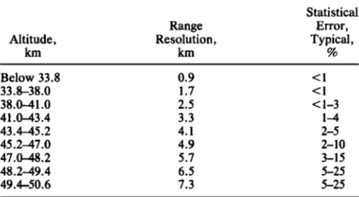
Table 1. Vertical Resolution and Typical Statistical Error

As a Function of Altitude Altitude, km Statistical Range Error, Resolution, Typical, km % Below 33.8 0.9 < 1 33.8-38.0 1.7 <1 38.0-41.0 2.5 <1-3 41.0-43.4 3.3 1-4 43.4-45.2 4.1 2-5 45.2-47.0 4.9 2-10 47.0-48.2 5.7 3-15 48.2-49.4 6.5 5-25 49.4-50.6 7.3 5-25

ozone profiles are therefore calculated, based on the high- and low-intensity data, which overlap in the region between approximately 25 and 40 km altitude. The high-intensity data

are saturated at low altitudes and the low-intensity data have poor signal-to-noise ratio at high altitudes. A composite

profile is then made up of the low-intensity data at low

altitudes and the high-intensity data at the higher altitudes.

The effects of saturation of the photon-counting system and the optimum altitude for the crossover from the low- to the

high-intensity data will be discussed in some detail later in this paper.

The system operates only at night and the signal is

averaged

for 10

6 laser

pulses,

which

takes

approximately

2

hours, to derive a single stratospheric ozone profile. The

ozone number density is obtained from the difference of the derivatives of the signals recorded for each wavelength, divided by the ozone differential absorption cross section,

taking into account the temperature dependence of this cross section. The slope (derivative) of the background corrected signal is computed as a function of range. As the altitude is

increased, the range resolution of the measurement has to be degraded to limit the increase in the statistical error related

to the rapid decrease in the signal level. To effect this compromise, the cutoff frequency of the low-pass derivative

filter is made to vary with altitude. The resulting altitude resolution and typical statistical errors are given in Table 1. Corrections to the raw data are made for the Rayleigh scattering and extinction terms, but no corrections for aero-

sols are made. The parameters required for the Rayleigh and temperature corrections are obtained from the COSPAR reference atmosphere monthly tables [Rees et al., 1990], interpolated to the correct latitude for Table Mountain

Facility (TMF). At this point in time, because of the low background level of aerosols in the stratosphere, this neglect

of aerosol corrections appears to have negligible influence on the derived ozone profile. In this particular lidar implemen-

tation the largest source of error has been found to be associated with the determination of the background signal. This important factor will also be discussed in detail below.

Results, Blind Intercomparison

The period of the official STOIC intercomparison ex-

tended for 14 days from July 20 through August 2, 1989. The JPL lidar made measurements during the 3 hours of darkness

preceding local (PDT) midnight, 0400-0700 UT, which then

allowed the GSFC lidar to operate from midnight until dawn. As we have described previously [McDermid et al., 1990c], it was not possible to operate the lidars simultaneously because the asynchronous observation of laser pulses from

the other system caused nonrandom fluctuations in the

background levels. The only exception to this timetable was on the final day, August 2, when a problem with one of the laser amplifiers delayed the start time of the JPL experiment

to 0930 UT. Ozone measurements were made for every night

of the intercomparison period although the atmospheric

conditions for lidar measurements were marginal on several of the nights.

For the blind intercomparison the complete lidar ozone

profiles, from 20 to 50 km altitude, were submitted and no data were excluded even when the signal-to-noise ratio of

the measurements was decreased because of clouds or poor

atmospheric visibility. Since comparison and review of the

blind data set allowed some improvements to be made to the

data analysis algorithm, this paper will concentrate on these modifications and comparisons with the final, refined results. However, it is appropriate to consider the results of the blind

intercomparison which indicated the areas where some

improvements were possible.

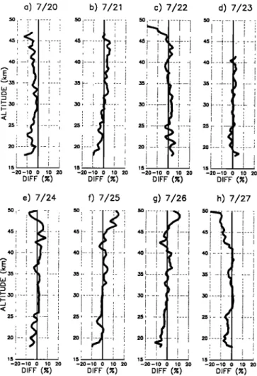
Figure 1 shows the average, and 1 •r standard deviation, of the 14 lidar ozone profiles from the blind data set. The large

standard deviations near the top of the profile, i.e., above

-•40 km, reflect the instrumental uncertainties at these

altitudes since the atmospheric variability in this region, over the period of the campaign, should be negligible. At

lower altitudes, below -•30 km, the instrumental uncertain-

ties are combined with a small degree of atmospheric vail-

ability that was observed by all of the instruments.

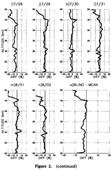
In Figures 2a-2m the lidar ozone profiles have been

compared, on a daily basis, to the average of all of the measurements made each day. The average of these daily

differences is then shown in the summary plot in Figure 20. In these and subsequent figures showing percentage differ-

ences in ozone, negative values denote lower ozone concen- trations measured by the lidar. Three significant features

were noted from this comparison. First, at 45 km the

50

...

30 .... d___/__LJ_ZJ_LLk ... L__2__L_LJ_LLLL ... L__ L_L_i_LZZ

25

1E+ 0 1E+11 1E+12 1E+13

OZONE NUMBER DENSITY (cm --'"3)

40

Figure 1. Mean (thick line) and 1 •r standard deviation (thin

lines) of the 14 JPL lidar profiles comprising the blind results

MCDERMID ET AL.' JPL STRATOSPHERIC OZONE LIDAR DURING STOIC 1989 9265

difference curve has an obvious inflection and the magnitude

of the difference starts to increase rapidly. Second, there is a small, consistent difference, of the order of 5ø/8, just above

30 km altitude where the high- and low-intensity profiles

were joined together. Third, the very first point, at 20 km altitude, was always low by approximately 10%. These three points were then carefully studied to see if there was a scientifically justifiable explanation and possible correction.

Refined Data Analysis

The problem identified at 20 km was caused by an error in

the data analysis algorithm that incorrectly considered the raw data at lower altitudes in calculating the derivative of the

signal at 20 km. This was readily corrected by starting the

analysis calculations at a lower altitude.

The original rationale for using high- and low-intensity

data to form a composite ozone profile was to avoid the need

to apply a saturation correction to the raw data counts. It

was apparent from the blind intercomparison that the high-

i)7/28

50

1

..._1•

....

• 50

•L•35

35

4s:•--..•

...

• ,•:i---•

4_,

' ' i

intensity data still showed a small degree of saturation immediately above the crossover point. There were two

potential

solutions

to this

problem.

The

first

was

to utilize

._.!

...

i--

0)7/20 b)7/21 c)7/22 d)7/23

"-'"'-"Z'.i

.-.ao ---• .... i no •... ,• .• ... i ... i 40: ... 2O_•o "•

"..:...I.."

""

_oo,o ,o i

,o ,o

•.-•

-•---i

BIFF

(%)

- •)IFF

(%)

BIFF

(%)

•35 "'i ... i 35f.. 351 ... f ... • 3si ... i ...

• ' : ' : '

' : : ' 't '

Figure

2.

(c nue

• 30 •- .... i ... [ ... ! 30 ': ... i ... i ... i 30 L ... i ... i ... 30 ': ...

251

ia,-4

...

25'---

i,

, i : 25'••

'..• 25'

...

'

...

' i

...

the

low-intensity

data

up

to

a

higher

altitude

were

it

was

20 -20-10 0 10 20 20 -20-10 0 10 20 20 -20-10 0 10 20 20 -20-10 0 10 20 approach was rejected because the signal-to-noise ratio of

DIFF (%) DIFF (%) DIFF (%) DIFF (%)

e)7/24

20

20

'•

20

i20

DIFF (%) DIFF (%) DIFF (%) DIFF (%)

Figure 2. Comparisons of the blind results set: (a)-(m)

Percentage difference of the Jet Propulsion Laboratory (JPL)

lidar profiles compared to the daily average of all of the blind

measurements. (o) Mean difference of the 14-day lidar aver-

age compared to the overall Stratospheric Ozone Intercom-

parison Campaign (STOIC) blind average.

the low-intensity data was falling rapidly and the errors in

the ozone concentration would be increased significantly in

this region. The second approach, which was adopted, was

to apply a correction for saturation or pulse pile-up caused

by the finite dead-time of the photon-counting system.

For the type of photon-counting system employed by the

lidar the system cannot register a second photon pulse until

a specific time interval has elapsed. This time interval is known as the dead time (•) and the counters will remain

paralyzed, i.e., will not register further photons, until a free

interval of at least the dead time has elapsed. This phenom-

enon is well known, has been extensively studied, and appropriate correction algorithms are available for a wide

variety of situations (see, for example, the following trea-

tises and references therein: Cantor and Teich [1975], Evans [1955], and Saleh [1978]).

Based on the Poisson characteristics of the photon-

counting process and the fact that this system can be paralyzed, then, as the true count rate increases, the ob-

served count rate, No, passes through a maximum given by

1

9266 MCDERMID ET AL.' JPL STRATOSPHERIC OZONE LIDAR DURING STOIC 1989 36 34 32 24 22 0 50 1 O0 150 200 250

SIGNAL (Normolized Photons/Pulse)

Figure 3. Effects of the photon-counting saturation correc-

tion on the raw data from the 308-nm high-intensity channel, for the July 20 experiment.

This relationship can be used to confirm the experimental

value for the dead time. The highest counts observed exper-

imentally were in the range 145-160 in a 4-/as time bin, which are equivalent to count rates of 36-40 MHz. Using these

values in (1) gives a range for the dead time of 9.2-10.1 ns or

a system specification of 100-108 MHz. The slowest com- ponents in the acquisition system are the multichannel scaler (MCS) and the pulse-height-discriminator which are speci- fied by the manufacturer at 100 and 110 MHz, respectively.

The observed maximum count rates are therefore in perfect

accord with these specifications which provides confidence

in assigning a dead time to use in the saturation correction

procedure.

The definition of the dead time forbids counts greater than

T/•' where T is the counting time interval, i.e., dwell time of the MCS, and thus the system will still reach saturation when the specified maximum rate of the system is reached. Below this level, the number of photons counted, Nc, as a function of the number actually received, Nr, is given by the formula

Nc = 1 + 1 - • Nr-1 exp-

(2)

As indicated above, the dead time was determined to be in the range 9.2-10.1 ns for the high-intensity 308-nm channel.

Since the other channels are not driven to saturation to the

same degree as this channel, it is not possible, under normal experimental conditions, to determine the dead time of each

channel individually from the raw data. Therefore it was

assumed that the dead time was constant for all channels,

and in order not to overcorrect the data the shorter dead time of 9.2 ns was used in the calculations. This is justifiable since

each channel is identical in terms of the types of photomul-

tipliers and signal detection electronics. Also, by testing the sensitivity of the derived ozone profiles to different values

for the dead time, it was found that no discernible differences

in the composite profile could be found for 10% variations of the dead time.

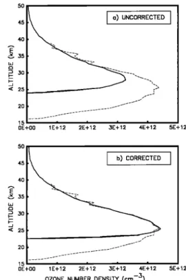
Equation (2) is inverted in order to obtain the true counts

as a function of the observed counts. Figure 3 shows the

effects of this correction procedure on the 308-nm high- intensity data recorded on July 20, the first day of STOIC.

The saturation correction does not become negligible until

an altitude of--•35 km. The correction procedure was applied

to all channels, including the low-intensity data. Figure 4

shows the dramatic effect of the saturation correction on the derived ozone profiles. The profile derived from the high- intensity data is shown by the solid line and that from the low-intensity data by the dashed line. The low intensity profile is unchanged by the saturation correction procedure, indicating that the signal intensity in these channels was low enough not to cause any pulse pile-up and that the correction algorithm does not induce changes when the data are not saturated. The ozone profile from the high-intensity data is unchanged only above --•35 km. Below this altitude the profile is changed significantly. As can be seen in Figure 4, the agreement between the high- and the low-intensity profiles is excellent and is extended downward to --•25 km which further gives confidence in the correctness of the saturation correction procedure. The profile derived from the high-intensity data has better signal to noise and hence

smaller statistical errors and it is therefore advantageous to

be able to move the crossover point for the composite profile to a lower altitude. The photon-counting system still reaches

a true saturation at --•100 MHz which is indicated by the

profile falling to zero immediately below the maximum. The low-intensity data were not saturated at all, but the effect of

45 < 25 20 15 OE+00 1E+12

I a)UNCORRECTED

I

2E•12 3E+12 4E•12 5E+12

40

<: 25

I b)

CORRECTED

OE+00 1E-•12 2E-•12 3E•12 4E+ 1

OZONE NUMBER DENSITY (cm -3)

5E+12

Figure 4. (a) Ozone profiles derived from the high- intensity (solid line) and low-intensity (dashed line) data

without saturation correction. These are blind results from

July 20 and the low to high crossover selected was at 32 km.

(b) The same profiles but with the saturation correction applied. These now constitute refined results. The low to

high crossover was at 28 km and the agreement between the

MCDERMID ET AL.' JPL STRATOSPHERIC OZONE LIDAR DURING STOIC 1989 9267

the electronic gates on the photomultipliers is shown by the

profile falling to zero at --•16 km. With the new analysis

procedure the ozone profile was extended down to 17 km,

limited by the electronic gates. These gates have since been

shifted to allow the lower limit of the profile to be extended down to 15 km.

At the upper end of the altitude range, the high-intensity data, and in particular the 308-nm channel, have been seen to be affected by a signal-induced noise [McDermid et al.,

1990d]. It has been determined that this is caused by the very

high intensity of laser radiation backscattered from the

boundary layer and the lower troposphere hitting the photo-

cathodes of the photomultiplier detectors. This signal is not

transmitted by the photomultiplier since it is electronically

gated off during this time, but the dark current of the tube shows a delayed recovery [Lee et al., 1990]. The effect of

this signal-induced noise is to increase and cause a curvature

of the background level. Different methods of fitting the

background have been studied [McDermid et al., 1990d; Iikura et al., 1987] and the best fit is given by a nonlinear

least squares exponential regression. The ozone profile

below --•40-45 km is insensitive to the method used to

estimate the background. However, above this altitude the profile is very sensitive to the background correction. For

the nonlinear exponential fit it is also found that the profile is

sensitive to the starting altitude of the regression. An impor-

tant factor in the background estimation is that the real signal

must be negligible at the starting altitude, but the fit must be started as low as possible in order to evaluate the curvature

correctly. Various methods have been used to select the

starting

altitude

and these

were reconsidered

in refining

the

data analysis. However, no suitable, justifiable modification

could be identified. For the final refined results, the back-

ground fitting for the 308-nm high-intensity channel was

started at 85 km for all data sets.

The only improvement in the agreement of the results

above 45 km was achieved by eliminating some of the

results. Based on consideration of the signal levels which were affected by clouds or other conditions, some of the

profiles were terminated at 47 km instead of 50 km. Table 2

Table 2. Atmospheric and Experimental Conditions

Relating to the Maximum Altitudes for the Profiles in the

Refined Results Set

Maximum Altitude, Date km Comment July 20, 1989 47 July 21, 1989 47 July 22, 1989 50 July 23, 1989 42 July 24, 1989 50 July 25, 1989 50 July 26, 1989 50 July 27, 1989 50 July 28, 1989 50 July 29, 1989 50 July 30, 1989 50 July 31, 1989 47 August 1, 1989 50 August 2, 1989 47

some high clouds, poor sky clarity

clouds toward end of experiment experiment terminated early due

to clouds

alignment problem

some high clouds

poor sky clarity (smoke haze) laser amplifier breakdown

o) 7/20 b) 7/21 c) 7/22 d) 7/2,3

,•5 -.:-. ,,• i ... •: ... i-- ,,• • .... i ... • ... J ,•5

40 40:- ... i ... i-- 40i ... ! ... i ... !

35

3•i

...

i

...

i-. 3•i

...

i ...

•

...

• 35

25 25 i ... i ... =;--- 25i ... • ... • ... i 25

2o 2oi ... i ... i ... •

20 "'i'"

15

15-20-10 0 10 20 -20-10 0 10 20 -20-10 0 10 20 -20-10 0 10 20

DIFF (%) DIFF (%) DIFF (%) DIFF (%)

e) 7/24 f) 7/25 g) 7/26 15 -20-10 0 10 2O DIFF (%) • 30 ... 1 -2O-lO o lO 20 5-2O-lO o lO 20 DIFF (%) DIFF (%) h) 7/27 , [ . ...• ... • 3si .... , . '. --,• 25 , 15 -20-10 0 1•3 20 DIFF (%) Figure 5. Same as Figure 2 but for comparisons of the refined results set. (a)-(m) Percentage difference of the JPL

lidar profiles compared to the daily average of all of the

refined measurements. (o) Mean difference of the 14-day

lidar average compared to the overall STOIC refined aver-

age.

shows

the dates,

maximum

altitudes

reached,

and commenis

on conditions affecting the experiment.

To minimize the error in the ozone concentration in the

upper range and to perform systematic reliable measure- ments at 50 km, mechanical gating of the photomultipliers

would be required.

Results, Refined Intercomparison

As for the blind data set, Figures 5a-5m shows the

difference of the JPL lidar profile compared with the average

of all profiles measured on a daily basis. The average of these

daily differences is shown in Figure 50. For this comparison

the mean difference of the lidar profiles from the average of

the other instruments is 4% or better from 18 to 48 km

altitude. In the region above 45 km the difference from the STOIC averages and the uncertainties in the lidar results start to increase rapidly. Because of the problems in evalu- ating and correcting for the background, which affects the profiles only in this region, the results obtained above 45 km

are of questionable value for trend detection even though

they agree within 10% with the STOIC results.

9268 MCDERMID ET AL.' JPL STRATOSPHERIC OZONE LIDAR DURING STOIC 1989 i) 7/28 15 -20-10 0 10 20 DIFF (%) j) 7/29 k) 7/30 I) 7/31 5o i .... 50 i .... ? ... • ,5o •.- -?. 45 45 •i'" 45 --- ß o ,m •o 35 35 35 ;50 ;50 ;50 2,5 25 25 2O 2O 20 15 -20-10 0 10 20 15 -20-10 0 10 ' 20 15_ 20-10 0 10 20

DIFF (%) DIFF (%) DIFF (%)

m) 8/01 n) 8/02 2s ... i ... 'i .... 25 ... i ... 20 20 ... 15 15-20-10 0 10 20 -20-10 0 10 20 DIFF (%) DIFF (%) o) REFINED ß MEAN , 15 -20 -10

DIFF

• (g) ,o

ment between the group of instruments but it should not be assumed that the average represents the true profile. There

are a number of biases in the average caused by the different altitude ranges and the different frequency of measurement for the various instruments. It is therefore valuable to also

consider one-to-one comparisons of the instruments. All of the lidar results have been compared with those from the other instruments on a profile-by-profile basis. This has revealed some systematic differences between individual instruments. There was only one day, July 24, when all instruments reported a profile and this date is therefore used as an example for these one-to-one comparisons. In the comparison plots that follow, Figures 6-11, the two lines that bracket the thick line on the difference plots represent the

limits of the combination of the quoted statistical error bars for each of the measurements [McDermid et al., 1990c]. If

the line of zero difference lies between these limits then the

measurements can be said to agree within the error bars (1 rr). This is not always the case, which therefore indicates the

presence of other error sources.

Figure 6a shows the refined profiles from the JPL and GSFC lidars for July 24, 1989. The JPL profile was recorded between 0440 and 0640 UT and the GSFC profile between

0751 and 1100 UT [McGee et al., this issue], both at TMF.

The percentage difference between these two profiles is

shown in Figure 6b. This comparison shows poorer agree- ment between the lidars than was generally observed during

STOIC and previously [McDermid et al., 1990c]. Since they

utilize the same technique and similar equipment, the two

lidars suffer the same problems, particularly with respect to signal-induced noise at high altitudes [McDermid et al.,

1990e; McGee et al., 1991]. Since the GSFC system has

slightly lower power than the JPL system, the background

50 45 40 30 25 2O a -- GL . LIDAR

'" -- JL

....

i ...

OZONE NO. DENSITY (cm- DIFFERENCE (%)

50 45 40 35n 30 25 20 20 30

Figure 6. Comparison of the refined profiles recorded by the JPL and the Goddard Space Flight Center

lidars on July 24. (a) Ozone concentration profiles. (b) Percentage difference between these profiles with

MCDERMID ET AL.' JPL STRATOSPHERIC OZONE LIDAR DURING STOIC 1989 9269 50 30 -

25

MICROWAVE

' ' '•I

1E+10 1E+11 1E+12 1E+13

OZONE

NO. DENSITY

(cm

-3)

40 50 45

-

30

<•

Figure 7. Comparison of the JPL lidar profile with that recorded by the Millitech/LaRC microwave radiometer for July 24. As Figure 6.

effects are typically seen at a lower altitude and this is reflected in the plots in Figure 6. Through the middle of the

range the agreement is very good, i.e., less than 5% differ- ence from -25 to 37 km altitude and less than 10% from the

start altitude of the GSFC profile at 20 km to -38 km altitude. In general, the range of good agreement, <10%,

extends from 20 km to above 40 km altitude.

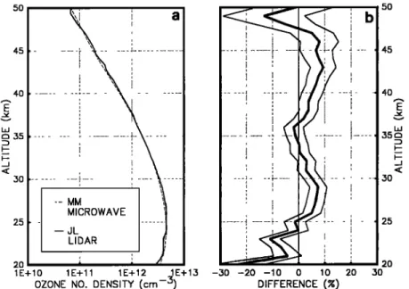
A comparison of the lidar profile with that measured by the Millitech/Langley Research Center (LaRC) microwave radiometer [Connor et al., this issue], averaged over the period 0400 to 1215 UT, is shown in Figure 7. Agreement to better than 10% over practically the entire range of the measurement is illustrated in Figure 7b. The somewhat sigmoid shape of

the difference curve was characteristic of all of the lidar-

microwave comparisons during STOIC and the lidar measure-

ment was always lower than the microwave near 20 km

altitude. The Millitech/LaRC microwave instrument continued

to operate at TMF through November 1989, following STOIC.

A more detailed comparison with the lidar over this extended

time period is given by Parrish et al. [ 1992].

The ROCOZ A rocket ozonesondes were launched from

San Nicolas Island, 33.3øN-119.5øW, and on July 24 the launch time was 1911 UT [Barnes et al., this issue]. As is

shown in Figure 8, above the ozone maximum the lidar to ROCOZ A difference is almost constant with the ROCOZ A

giving an ozone concentration -5% higher than the lidar.

This may be a characteristic of the ROCOZ A instrument

[Barnes et al., 1989] although the agreement seen during the October-November 1988 intercomparison was better [Mc-

Dermid et al., 1990b].

SAGE II made a sunrise measurement at 1317 UT, July

24, and at a tangent point 31.2øN-120.7øW which is 536 km

5O 45 40 • 35 30 25 20

1E+10

1E+11

1E+12

J)E+13

5O

- . 45

9270 MCDERMID ET AL.' JPL STRATOSPHERIC OZONE LIDAR DURING STOIC 1989 Figure 9. Figure 6. 50 45 40 •_ 30 25 20 15 1E+ -- SA SAGE II --JL LIDAR 1E+11 1E+12

•

50

...

i

...

45

.--'i!--

.]

20

OZONE

NO.

DENSITY

(cm

-3)

DIFFERENCE

(%)

Comparison of the SAGE II satellite measurement with the JPL lidar profile for July 24. As

from TMF. The agreement between the lidar and the SAGE

II profiles, Figure 9a and 9b, is excellent showing <5%

difference

from the ozone

maximum

to above

40 km (i.e.,

---2d •.4 km) where the lidar data signal-to-noise ratio starts to fall. This is typical of the agreement seen between the JPL

lidar and the SAGE II over an extended period for SAGE II

measurements made within 1000 km of TMF [McDermid et al., 1990a]. However, below the ozone maximum the two

profiles start to diverge with the lidar data typically showing lower ozone concentrations than SAGE II, similar to the

comparison with the microwave radiometer.

In Figures 10 and 11 the lidar results are compared with those obtained from the balloon ECC sondes launched by the National Oceanic and Atmospheric Administration

(NOAA) [Komhyr et al., this issue] and by Wallops Flight

Facility (WFF) [Barnes and Torres, this i•sue]. On July 24

the WFF sonde was launched at 0546 UT and the NOAA

sonde at 0559 UT, both from TMF. In Figures 10a and 1 l a the ozone number density axis has been changed to a linear scale which shows more clearly the structure in the ozone profile at the lower altitudes. Because of the relatively slow ascent rate of the balloons the vertical resolution of the ECC measurements is the best of all of the instruments in STOIC. Small features were observed in the ozone profile by the sondes and these are reproduced, with only minimal smooth-

ing, by the lidar. The agreement in the values obtained for

the ozone concentration as well as in the shape of the profile is also good except for the first point of the lidar profile.

30 28 26

•, 22

OZONE

NO.

DENSITY

(cm

-3)

30 .. 28 20 -': - - ' 16 -30 -20 -10 0 10 20 30 DIFFERENCE (%)

Figure 10. Comparison of the JPL lidar profile with that recorded by the NOAA electrochemical concentration cell balloon sonde on July 24. As Figure 6. Note the features in the ozone profile in this altitude range that are observed by both instruments (compare Figure 11).

MCDERMID ET AL.' JPL STRATOSPHERIC OZONE LIDAR DURING STOIC 1989 9271 30 --JL .. LIDAR .

ß I/"• .

OZONE NO. DENSITY (cm -3)

• 22 20 30 20 18 16 -30 -20 -10 0 10 20 30 DIFFERENCE (%)

Figure 11. Comparison of the JPL lidar profile with that recorded by the Wallops Flight Facility ECC balloon sonde on July 24. As Figure 6. Note the features in the ozone profile in this altitude range that are observed by both instruments (compare Figure 10).

Summary

STOIC has represented a very important stage in the development of the differential absorption lidar for its pro- posed role in the NDSC and for correlative measurements with the Upper Atmosphere Research Satellite (UARS) and other satellite programs. It has provided a unique opportu-

nity to test some of the alternative procedures in the data

analysis and has allowed the ozone concentration profile algorithm to be improved. The need for hardware modifica- tions to reduce the effects of signal-induced noise on the high-altitude measurements was also indicated.

It is believed that this study confirms the power of the DIAL technique for making accurate measurements of stratospheric ozone concentration profiles on a regular and

long-term basis. The JPL lidar, in its present implementa-

tion, has shown agreement with the STOIC average to better

than 4% from 18 to 48 km altitude. The results above 45 km

altitude are subject to the greatest uncertainty and error and are of questionable value even though they agree within 10%

with the STOIC average. The lidar compared well with other

techniques and appears capable of providing reliable and reproducible results. Studies such as STOIC and intercom- padsons with other instruments should continue as an on- going check on the various sensors and to provide validation in the determination of long-term changes.

Acknowledgments. The work described in this paper was carried out at the Jet Propulsion Laboratory, California Institute of Tech- nology, under a contract with the National Aeronautics and Space Administration. We are grateful to the many other participants in the STOIC campaign for their cooperation and for sharing their results.

References

Barnes, R. A., and A. L. Torres, Electrochemical concentration cell

ozone soundings at two sites during the STOIC campaign, J. Geophys. Res., this issue.

Barnes, R. A., M. A. Chamberlain, C. L. Parsons, and A. C.

Holland, An improved rocket ozone sondes (ROCOZ A), 3,

Northern midlatitude ozone measurements from 1983 to 1985, J. Geophys. Res., 94, 2239-2254, 1989.

Barnes, R. A., C. L. Parsons, and A. P. Grothouse, ROCOZ A

ozone measurements during the Stratospheric Ozone Intercom- parison Campaign (STOIC), J. Geophys. Res., this issue. Cantor, B. I., and M. C. Teich, Dead-time-corrected photo-counting

distributions for laser radiation, J. Opt. $oc. Am., 65, 786-791,

1975.

Connor, B. J., A. Parrish, J.-J. Tsou, and M.P. McCormick, Error

analysis for the ground-based microwave ozone measurements during STOIC, J. Geophys. Res., this issue.

Evans, R. D., The Atomic Nucleus, chap. 28, Applications of Poisson Statistics to Some Instruments Used in Nuclear Physics,

McGraw-Hill, New York, 1955.

Iikura, Y., N. Sugimoto, Y. Sasano, and H. Shimizu, Improvement on lidar data processing for stratospheric aerosol measurements, Appl. Opt., 26, 5299-5306, 1987.

Komhyr, W. D., R. A. Barnes, J. A. Lathrop, G. B. Brothers, and D. P. Opperman, Electrochemical concentration cell ozonesonde performance evaluation during STOIC 1989, J. Geophys. Res.,

this issue.

Lee, H. S., G. K. Schwemmer, C. L. Korb, M. Dombrowski, and C. Prasad, Gated photomultiplier response characterization for DIAL measurements, Appl. Opt., 29, 3303-3315, 1990.

Margitan, J. J., et al., Stratospheric Ozone Intercomparison Cam- paign (STOIC) 1989: Overview, J. Geophys. Res., this issue. McDermid, I. S., A 4-year climatology of stratospheric ozone from

lidar measurements at Table Mountain, 34.4øN, J. Geophys. Res.,

98, 10,509-10,515, 1993.

McDermid, I. S., and S. M. Godin, Stratospheric ozone measure- ments using a ground-based, high-power lidar, laser applications in meteorology and Earth and atmospheric remote sensing, Proc.

$PIE Int. $oc. Opt. Eng., 1062, 225-232, 1989.

McDermid, I. S., S. M. Godin, P. H. Wang, and M.P. McCormick, Comparison of stratospheric ozone profiles and their seasonal variations as measured by lidar and Stratospheric Aerosol and Gas Experiment during 1988, J. Geophys. Res., 95, 5605-5612,

1990a.

McDermid, I. S., et al., Comparison of ozone profiles from ground-

based lidar, electrochemical concentration cell balloon sonde,

ROCOZ A rocket ozone sondes, and Stratospheric Aerosol and Gas Experiment satellite measurements, J. Geophys. Res., 95,

10,037-10,042, 1990b.

McDermid, I. S., S. M. Godin, L. O. Lindquist, T. D. Walsh, J.

9272 MCDERMID ET AL.: JPL STRATOSPHERIC OZONE LIDAR DURING STOIC 1989

Measurement inter-comparison of the JPL and GSFC strato- spheric ozone lidar systems, Appl. Opt., 29, 4671-4676, 1990c. McDermid, I. S., S. M. Godin, and L. O. Lindquist, Ground-based

laser DIAL system for long-term measurements of stratospheric ozone, Appl. Opt., 29, 3603-3612, 1990d.

McDermid, I. S., S. M. Godin, and T. D. Walsh, Lidar measure- ments of stratospheric ozone and intercomparisons and valida- tion, Appl. Opt., 29, 4914-4923, 1990e.

McGee, T. J., P. Newman, R. Ferrare, D. Whiteman, J. Butler, J. Burris, S. M. Godin, and I. S. McDermid, Lidar observations of ozone changes induced by subpolar air mass motion over Table Mountain (34.4 ø N), J. Geophys. Res., 95, 20,527-20,530, 1990. McGee, T. J., D. Whiteman, R. Ferrare, J. Butler, and J. Burris,

STROZ LITE: NASA/GSFC Stratospheric Ozone Lidar Trailer Experiment, Opt. Eng., 30, 31-39, 1991.

McGee, T. J., R. A. Ferrare, D. N. Whiteman, J. J. Butler, J. F.

Burris, and M. A. Owens, Lidar measurements of stratospheric ozone during the STOIC campaign, J. Geophys. Res., this issue.

Rees, D., J. J. Barnett, and K. Labitzke (eds.), COSPAR Interna-

tional Reference Atmosphere: 1986, II, Middle Atmosphere Mod- els, Adv. Space Res., 10, 1-517, 1990.

Saleh, B., Photoelectron Statistics, Springer Ser. Opt. Sci., vol. 6, edited by D. L. MacAdam, Springer-Verlag, New York, 1978. Upper Atmosphere Research Program (NASA-UARP), Network for

the Detection of Stratospheric Change, report of the Workshop, Boulder, Colorado, March 5-7, 1986.

S. M. Godin, I. S. McDermid, and T. D. Walsh, Jet Propulsion Laboratory, Table Mountain Facility, P.O. Box 367, California Institute of Technology, Wrightwood, CA 92397-0367.

(Received April 16, 1993; revised August 15, 1994; accepted August 15, 1994.)