Interest of a Full-Waveform Flown UV Lidar to Derive Forest Vertical Structures and Aboveground Carbon

HAL Id: hal-02902901

https://hal.archives-ouvertes.fr/hal-02902901

HAL is a multi-disciplinary open access archive for the deposit and dissemination of sci-entific research documents, whether they are pub-lished or not. The documents may come from teaching and research institutions in France or abroad, or from public or private research centers.

L’archive ouverte pluridisciplinaire HAL, est destinée au dépôt et à la diffusion de documents scientifiques de niveau recherche, publiés ou non, émanant des établissements d’enseignement et de recherche français ou étrangers, des laboratoires publics ou privés.

Forest Vertical Structures and Aboveground Carbon

Xiaoxia Shang, Patrick Chazette

To cite this version:

Xiaoxia Shang, Patrick Chazette. Interest of a Full-Waveform Flown UV Lidar to Derive For-est Vertical Structures and Aboveground Carbon. Forests, MDPI, 2014, 5 (6), pp.1454-1480. �10.3390/f5061454�. �hal-02902901�

forests

ISSN 1999-4907

www.mdpi.com/journal/forests

Article

Interest of a Full-Waveform Flown UV Lidar to Derive Forest

Vertical Structures and Aboveground Carbon

Xiaoxia Shang * and Patrick Chazette

Laboratoire des Sciences du Climat et l’Environnement, Commissariat à l’Energie Atomique et aux Energies Alternatives—Centre National de la Recherche Scientifique—Université de Versailles Saint-Quentin-en-Yvelines, Gif sur Yvette Cedex 91191, France; E-Mail: patrick.chazette@lsce.ipsl.fr

* Author to whom correspondence should be addressed; E-Mail: xiaoxia.shang@lsce.ipsl.fr;

Tel.: +33-1-6908-7889; Fax: +33-1-6908-7716.

Received: 12 December 2013; in revised form: 22 April 2014 / Accepted: 10 June 2014 / Published: 20 June 2014

Abstract: Amongst all the methodologies readily available to estimate forest canopy and

aboveground carbon (AGC), in-situ plot surveys and airborne laser scanning systems appear to be powerful assets. However, they are limited to relatively local scales. In this work, we have developed a full-waveform UV lidar, named ULICE (Ultraviolet LIdar for Canopy Experiment), as an airborne demonstrator for future space missions, with an eventual aim to retrieve forest properties at the global scale. The advantage of using the UV wavelength for a demonstrator is its low multiple scattering in the canopy. Based on realistic airborne lidar data from the well-documented Fontainebleau forest site (south-east of Paris, France), which is representative of managed deciduous forests in temperate climate zones, we estimate the uncertainties in the retrieval of forest vertical structures and AGC. A complete uncertainty study using Monte Carlo approaches is performed for both the lidar-derived tree top height (TTH) and AGC. Our results show a maximum error of 1.2 m (16 tC ha-1) for the TTH (AGC) assessment. Furthermore, the study of leaf effect on AGC estimate for mid-latitude deciduous forests highlights the possibility for using calibration obtained during only one season to retrieve the AGC during the other, by applying winter and summer airborne measurements.

Keywords: airborne lidar; full-waveform UV lidar; forest vertical structures; aboveground

1. Introduction

Deforestation or degradation of forest accounts for about 20% of total global emissions of carbon dioxide (CO2) and thus significantly contributes to climate change [1]. Gibbs et al. [2] pointed out that the majority of carbon is sequestered in aboveground live tissues (e.g., trees). A strong relationship between the stand height and the stand biomass occurs [3], which highlights the need to develop tools for the assessment of tree height at the global scale. Traditionally, the aboveground biomass (AGB, in g ha-1) and the aboveground carbon (AGC, in gC ha-1, based on the biomass to carbon conversion factor 0.5) have been assessed using field-based inventory plots and from aerial photography. More recently, airborne (e.g., [4–7]) or spaceborne (e.g., [8–13]) lidar systems have demonstrated the possibility to characterize the three-dimensional distribution of biomass elements of forest canopies and, furthermore, to estimate the AGB or AGC. Moreover, IPCC [1] provided guidelines to assist countries in the development of carbon-assessment methodologies, amongst which lidar is a powerful candidate to monitor forests at both regional and global scales. The recent publication of Zolkos et al. [14] concluded that lidar metrics may be significantly more accurate than those using radar or passive optical data; hence, the establishment of relationships between forest stand attributes and lidar measurements is a pertinent approach with which to assess the AGB or AGC over a wide range of spatial scales (e.g., [15]). Nevertheless, the complementarity between lidar and radar could be an advantage when designing a space mission because they are neither sensitive to the same biomass account nor based on the same interaction between the emitted radiative wave and the forest. The use of a P-band radar by the European Space Agency (ESA) [16] opens a new perspective for the conduct of forest surveys from space and could be further improved by a synergy with lidar measurements.

Airborne laser scanning systems appear to be powerful assets for forest studies. However, they are limited to relatively local scales. Airborne measurements using a large-footprint lidar are more promising for studies of forest landscapes at larger scales [17]. We have developed such a lidar system to meet the need of an airborne demonstrator for possible future space missions, with an eventual aim to retrieve the forest properties at the global scale. This article is mainly dedicated to the data analysis approach with which to measure both the forest vertical structures and the AGC, and to the assessment of the relative uncertainties involved in this. It is based on measurements performed by a full-waveform ultraviolet (UV) airborne lidar over a deciduous mid-latitude forest, which has been selected to give realistic and representative samples. The synergy between multispectral measurement instruments, radar and lidar could further improve the uncertainties presented here, but this is beyond the scope of the present work.

The description of the instrumental setup and the experimental strategy is given in Section 2. In Section 3, we present algorithms developed for the retrieval of the tree top height (TTH) and the quadratic mean canopy height (QMCH) from the full-waveform UV lidar profiles. We also show how the lidar has been calibrated and applied for constituting a realistic sampling of the AGC at a spatial resolution compatible with the forest stand scale. In Section 4, the results and main uncertainty sources are fully discussed. The effect of leaves on both the forest vertical structures and the AGC are also discussed in Section 4.

2. Instrumental Set-Up and Strategy

The new custom-built ultraviolet (UV) lidar ULICE (Ultraviolet LIdar for Canopy Experiment) payload was embedded on an Ultra-Light Aircraft (ULA) to allow rapid deployments and flight plans flexibility over the sampling sites. This system is an airborne prototype for future space missions designed to study forests at the global scale and has been specially developed for these demonstration experiments. Compared to the near infrared (NIR) lidar systems that are generally considered for canopy studies, the use of the UV spectral domain leads to a significant reduction of the multiple scattering effect within the forest structures, because of the lower reflectance by the vegetation at these wavelengths [18]. Considering a spaceborne lidar mission, the use of UV will lead to disadvantages due to atmospheric transmission, since the atmospheric optical thickness at UV wavelengths is about five times larger than at NIR wavelengths. However, increasing the emitted laser energy can compensate for this attenuation. Besides, this drawback is negligible for our low-altitude airborne lidar measurements because the atmospheric transmission is close to 0.98. Hence, an airborne UV lidar is a good candidate to be a reference for a spaceborne lidar.

It should be mentioned that two space missions will board a UV lidar in the near future: (1) The ESA (European Space Agency)/JAXA (Japan Aerospace Exploration Agency) mission EarthCare (Earth Clouds, Aerosols and Radiation Explorer) will board an Atmospheric Lidar (ATLID) [19,20]; (2) The ESA mission ADM-Aeolus (Atmospheric Dynamics Mission Aeolus) will board the Atmospheric Laser Doppler Instrument (ALADIN) [21,22].

2.1. ULA Carrier

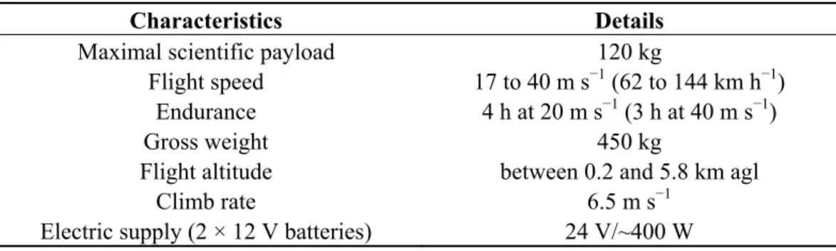
The ULA used in this study is a pendular ULA model Tanarg 912S with BioniX 15 wings manufactured and marketed by the Air Creation company ([23], Table 1). It is equipped with a Rotax 912S100-hp motor with a 72 dB noise impact at 150 m from the surface and full power (Figure 1). It is also equipped with a VHF radio with a bandwidth of 25 kHz and Mode S transponders. During this study it flew at about 300 m above ground level (agl) with a velocity of ~20 m s−1. This carrier has been selected because of its flexibility to perform lidar measurements over small and medium areas [24]. It also has the capability to take off from small airfields. The ULA maneuverability provides the ability to quickly double-back above the same site, and therefore make an exhaustive horizontal sampling. It is a good candidate to collect the required data set, and so perform a comprehensive demonstration study on forest properties derived from a full-waveform UV lidar.

Table 1. Main characteristics of the ULA a.

Characteristics Details

Maximal scientific payload 120 kg

Flight speed 17 to 40 m s−1 _{(62 to 144 km h}−1₎ Endurance 4 h at 20 m s−1 _{(3 h at 40 m s}−1₎

Gross weight 450 kg

Flight altitude between 0.2 and 5.8 km agl

Climb rate 6.5 m s−1

Electric supply (2 × 12 V batteries) 24 V/~400 W

Figure 1. ULICE (Ultraviolet LIdar for Canopy Experiment) onboard an ULA (Ultra-Light

Aircraft). The lidar optical head is shown on the left picture. The top right picture shows a global view of the lidar embedded on the ULA. The bottom right picture shows the lidar in flight during the experiment, with the optical head pointing downward.

2.2. Scientific Payload

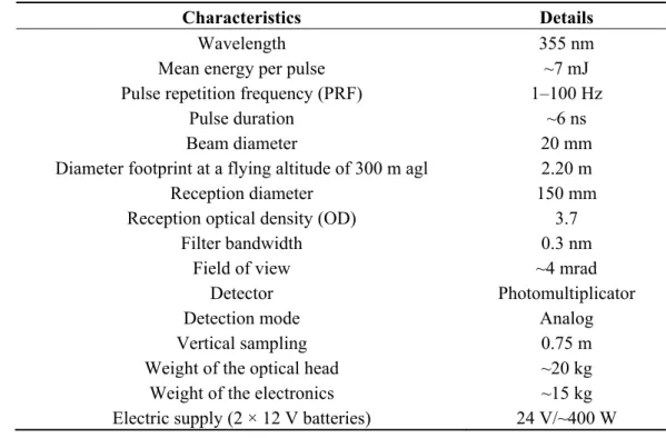
The main instrument is the homemade canopy lidar ULICE (Figure 1), which has been developed by LSCE (Laboratoire des Sciences du Climat et l’Environnement, France) for scientific studies. ULICE operates at eye-safe conditions from the emission of the optical head. It uses a Centurion laser (a diode-pumped Nd-YAG solid state laser) manufactured by the Quantel company [25], operating at 355 nm and delivering 7 mJ energy in 6 ns at the pulse repetition frequency (PRF) of 20 Hz (Table 2). At the 20 m s−1 ULA flight speed, the successive lidar shot centers are separated by ~1 m. The laser energy is deliberately oversized, which is compensated by optical densities (OD = 3.7) at the reception, in order to reduce the contribution of the sky radiance. The full-waveform lidar signal is digitized at a 200 MHz sampling frequency by a high-speed digitizer card NI-PXI-5124 manufactured by the National Instruments Company [26]. This yields a 0.75 m sampling resolution along the lidar line of sight, well adapted for a mid-latitude forest of 20~30 m in height.

The laser beam is emitted downwards to the forest in the near nadir direction (<10° from nadir). Small-footprint results in a higher PRF, while large-footprint systems increase the probability to hit both the ground and the canopy top simultaneously. Our footprint diameter was a compromise value between the small- and large-footprint diameters as in Cuesta et al. [6]. The beam divergence of the lidar was set up to 4 mrad, yielding to laser footprints at ground level of ~2 m in diameter. The TTH retrieval using such a footprint size is hardly influenced by the surface slopes encountered at the sampling sites.

Table 2. Characteristics of the ULICE a.

Characteristics Details

Wavelength 355 nm

Mean energy per pulse ~7 mJ

Pulse repetition frequency (PRF) 1–100 Hz

Pulse duration ~6 ns

Beam diameter 20 mm

Diameter footprint at a flying altitude of 300 m agl 2.20 m

Reception diameter 150 mm

Reception optical density (OD) 3.7

Filter bandwidth 0.3 nm

Field of view ~4 mrad

Detector Photomultiplicator

Detection mode Analog

Vertical sampling 0.75 m

Weight of the optical head ~20 kg Weight of the electronics ~15 kg Electric supply (2 × 12 V batteries) 24 V/~400 W

a _{ULICE, Ultraviolet LIdar for Canopy Experiment.}

An ancillary positioning instrument, called the MTi-G system, and manufactured by the XSENS company [27] is also onboard the ULA (Table 3). It provides the position and the attitude information of the ULA (Euler angles: yaw, pitch and roll) necessary to derive the angle between the actual lidar line of sight and the nadir direction. The Global Positioning System (GPS) and the Attitude and Heading Reference System (AHRS) are part of the MTi-G system. The 20–Hz GPS measurements tracked the ULA position with an accuracy of 5 m (MTi-G leaflet, [27], Table 3). The AHRS consists of sensors on three axes that provide the three Euler angles with 0.7° accuracy (i.e., 3.6 m at the ground for a flight altitude of 300 m agl). A discussion on the influence of the lidar footprint position and its associate uncertainties will be presented later.

Table 3. Technical specifications of the ancillary instrument (MTi-G).

Characteristics Details

GPS

Receiver type 50 channels L1 frequency; C/A code Galileo L1; Open Service

GPS update rate 4 Hz

Start-up time cold start 29 s

Tracking sensitivity −160 dBm

Timing accuracy 50 ns RMS

AHRS

Static accuracy (roll/pitch) <0.5 deg Static accuracy (heading) <1 deg

Dynamic accuracy 1 deg RMS

Angular resolution 0.05 deg

Dynamic range: -Pitch

-Roll/Heading

±90 deg ±180 deg

2.3. Forest Sites and Sampling Strategy

The main challenge for forest studies at the global scale is the AGC assessment. Tropical forests are known as the main reservoir of carbon and are difficult to penetrate by laser beam due to their high density. For this initial scientific study we did not have the opportunity to perform airborne measurements over such a tropical forest. Thus, deciduous forests in France have been sampled for a first test of the UV lidar interest.

We performed airborne lidar experiments over the deciduous forest of Fontainebleau. This forest of ~17,000 ha (48°25′ N, 2°40′ E) is located 60 km south-east of Paris (Figure 2). It is a managed mature oak forest with a dense understory of coppiced hornbeams. It is well documented by the Office National des Forêts (ONF, [28]). Fontainebleau is representative of the managed oak that occupies about 31% of the total surface of French forests. Moreover, oaks are widely distributed from central Spain to Norway in Europe. The forest is of flat topography and lies at ~120 m above mean sea level (amsl). The climate is temperate, subject to the influence of both oceanic effects from the west and continental effects from the east. The mean annual temperature is 10.6 °C and the mean annual rainfall is 750 mm [29].

Figure 2. Location of the sampling sites, both of them site in the Fontainebleau Forest

(48°25′ N, 2°40′ E, south-east of Paris) in the region of Ile de France of France (map of forest areas from: [30]). Site 1 is close to the northeastern part of the Fontainebleau forest, Site 2 at the western end.

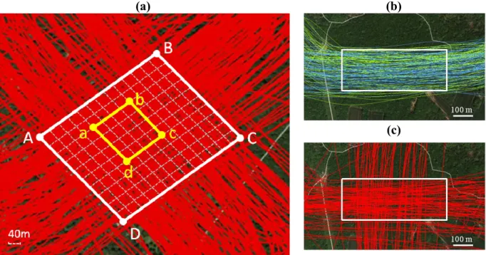
Two sampling sites were selected inside the Fontainebleau forest for a total of 30 days of measurements. Site 1, of ~20 ha (Figure 2), was first sampled during the winter of 2010, in order to avoid signal attenuation by canopy leaf strata and the effects of the ground cover vegetation. An exhaustive horizontal sampling was performed (Figure 3a) for comparison with detailed field measurements made by ONF five years previously (2005) over an area of 2.6 ha in the middle of the site. Site 2, of ~11 ha, (Figure 2, Figure 3b,c) was sampled both during summer 2012 and winter 2012–2013, so as to study the leaf effect on estimates of both the forest vertical structures and the AGC. This site was not subject to any harvesting between our two lidar experiments.

Figure 3. Flight tracks superimposed in color over the sampling sites (GoogleTM Earth). (a) Site 1 is at the crossing of winter 2010 flight tracks within the white rectangle ABCD. The well-documented central area is highlighted in the yellow rectangle abcd. The forest plots of 40 m × 40 m are bounded by white-gray dotted lines; (b) Flight tracks over the Site 2 in summer 2012; (c) Flight tracks over the Site 2 in winter 2012–2013.

(a) (b)

(c)

The sampling strategy has been elaborated from previous studies above the “Landes” forests [6,7]. The horizontal resolution is driven by the laser PRF, the ULA’s ground speed and the laser divergence; its mean value has been computed using a set of footprints randomly spread in the sampling site and found to be ~2 m.

3. Theory

Lidar backscatter profiles include a signature from vertical forest structures, which is dominant compared to the atmospheric contribution. Hence, the TTH can be extracted from the lidar profile [6]. However, the entire lidar profile within the canopy, bounded by the TTH, is also key information with which to derive the AGC from the quadratic mean canopy height (QMCH) as defined by Lefsky et al. [31]. Hereafter, the inversion methodology is entirely described before estimating the uncertainty sources and magnitudes. We can distinguish two main steps. The first step, to retrieve the

TTH and QMCH, is only dependent on the lidar measurements, whilst the second, to retrieve the AGC, needs exogenous material extracted from the scientific forestry literatures.

3.1. Tree Top Height (TTH) Retrieval from Lidar Measurements

The TTH is calculated as the distance between the first return at the upper surface of the vegetation and the last return from the ground surface. In order to retrieve forest vertical structures, it is necessary to detect the intensity peaks of both the canopy and ground echoes in the full-waveform lidar signals. A similar method has been used in atmospheric studies for the identification of clouds by Chazette et al. [32]. This algorithm has been significantly improved by using a sensitivity approach to retrieve the different values of thresholds.

The method is composed of two threshold steps. The first is the detection of the ground echo compared to the noise level, which can be inferred from the signal remaining after the ground echo when only the instrumentation noise exists (Figure 4). The noise is thus calculated beneath the undershot linked to the quick transition associated with the ground echo. The second step is the detection of the canopy echo, considering the atmospheric signal just above the trees (Figure 4).

Figure 4. Typical example of a lidar profile measured over a sampling site. The two

thresholds used to detect the ground echo (GE) and the canopy echo (CE) are represented in red and blue, respectively.

The ground echo (GE) is defined from the last echo peak of a lidar profile (the furthest from the laser emission), while the signal of the canopy echo (CE) is identified as all return lidar signals above the GE. Both the GE and the CE are defined by inequalities on the lidar signal S by:

(1) where and are the mean value and the standard deviation of SN (the noise signal), respectively,

under the ground level for the GE (x = GE) and above the canopy top for the CE (x = CE). CGE and

CCE are coefficients that are optimized by seeking the minimum relative residue on the mean tree top

height (MTTH) retrieval following an iterative approach. Note that the lidar GE waveform should be calibrated by using the return laser pulse in the nadir/zenith direction over a flat surface such as the tarmac of the aerodrome from where the ULA took off.

After retrieval of both the GE and CE, the lidar-derived TTH was obtained for each lidar profile (i.e., the distance between the blue and the red crosses in Figure 4). However, owing to the ULA attitude, the laser beam is not always emitted with a perfect nadir direction and so a distortion may be observed on the retrieved TTH. Moreover, the location of the laser footprint can also be affected by the ULA attitude. So the TTH and the location of the footprint have to be corrected as described in Appendix A.

3.2. Quadratic Mean Canopy Height (QMCH) Retrieval from Lidar Measurements

With the ULICE system, individual trees cannot be distinguished because of the footprints overlaps—a higher accuracy of geolocation would be required to do so. However, our research focuses on the carbon estimation for statistically representative plot sizes of forest properties. Lidar profiles after correction of the ULA attitude in each given plot are then averaged, and the QMCH was introduced to determine a better correlation between lidar measurements and field-derived carbon, as described in Lefsky et al. [31].

The transmittance height profile (THP) is estimated between the GE and the CE (TTH), from the average lidar signal in the plot, by taking the ratio of the energy from canopy returns (Eh) to the total

energy (E0) (Equation 2), which also amounts to the fraction of the sky covered by canopy. Hence the THP can be explained for a flight altitude agl zf by:

(2)

where:

(ℎ) =_{( − ℎ)} ∙ (ℎ) ∙ exp −2 ( ) ∙ ₍₃₎

with C the lidar instrumental constant, α the extinction coefficient, and β the backscattering coefficient [33].

The THP can be considered as the cumulative probability density function that a photon does not reach level h after crossing the canopy between TTH and h. Note that multiple scattering within the canopy may affect this consideration. Nevertheless, we do not consider it here as we operate on the UV

    ⋅ + > ⋅ + > N CE CE N CE N GE GE N GE C S S C S S σ σ N x S N x σ

(

)

(

)





wavelength and are less sensitive to the multiple scattering effects. Therefore, the probability density function (PDF) that a photon coming from the level h is scattered at the level h-dh can be expressed as:

(4) where CHP is the canopy height profiles as defined in Lefsky et al. [31]. This is also the PDF defining the fraction of sky covered by canopy between the levels h and h-dh. From Equation (4), we find that:

(5) The ULICE system cannot distinguish various scattering sources, so CHP characterizes the surface area of all canopy material (foliar and woody). When integrating Equation (5), the cumulative CHP (CCHP) between h and TTH, as described by the MacArthur Horn equation [34] and used for airborne and/or spaceborne lidar measurements by several authors (e.g., [31,34]), can be derived as:

(6) By using CHP, we can also express both the mean canopy height (MCH) and the QMCH as:

(7)

Lefsky et al. [31] have pointed out that, amongst several studied variables, the QMCH is the most highly correlated with the AGB or AGC. Nevertheless, the assessment of the QMCH requires the prior assessment of the TTH. Note that the lidar-derived QMCH and MCH are in good agreement (not shown) and that it would be equivalent to use one or the other for the AGB or AGC retrieval. To preserve the coherence with previous authors, we hereafter used only the QMCH to assess the AGC.

3.3. Aboveground Carbon (AGC) Retrieval from Field Measurements

Allometric equations that relate the AGC of forests to the stem dimensions are almost universally used [4,5,13,17,31,35]. The assessment of the AGC for each documented tree (AGCt) requires the

knowledge of its total volume (Vtot), which is defined as the volume of all aerial living woody parts,

including small branches and twigs. The tree top height (TTH) and the circumference at breast heights (CBH) are required to calculate the total volume.

Generally, the CBHs are more likely to be available; the TTHs are then assessed from a non-linear monotonically increasing relationship between TTH and CBH. This allometric law (also called “heights curve”) is widely applied to calculate the average and the dominant TTH. Among the commonly used models, the hyperbolic model of De Dhôte and De Hercé [36] seems more robust and better adapted to the geometry of the heights-circumferences dispersion. The initial model is used for beeches and oaks. It gives TTH (in m) against CBH (in cm) as follows:

(8)

(

)

(

) (

)

(

)

(

)





where µ1, µ2 and µ3 are coefficients to be adjusted.

Hereafter the allometric relationships given in Vallet et al. [37] have been used to derive Vtot and

then AGCt. Vtot (in m3) of each tree can be calculated by using a total volume equation, which is

expressed by CBH (in cm) and TTH (in m) as:

(9) where ξ(CBH,TTH) is the ratio between the tree’s volume and that of a cylinder of similar height and circumference. Its mathematical model reads as follows:

(10) where α, β and γ are the coefficients adjusted for tree species, and ε is the model’s residual. AGCt (in

tC tree−1) for each individual tree has then been computed as:

(11) where DEN is the basic density for the species, and CAR is the proportion of carbon in the dry matter. Hence, AGCt derived from field measurements has been calculated to assess the plot-level AGC in

the documented area, which has been divided into plots of a predefined size. The GPS used during the field measurements brings an uncertainty on the n trees’ locations. For this reason, the plot-level AGC (AGCplot given in tC ha−1) has been derived from the contributions of each AGCt weighted by the PDF

W that trees fall in the considered plot as:

(12) where W is a function of latitude (λ) and longitude (φ), and Splot (in m2) is the predefined plot surface.

3.4. AGC Estimation via QMCH

Following the work of Lefsky et al. [31], a linear regression can be established between the plot-level QMCH and field-derived AGCplot as

(13) where a and b are the coefficients to be adjusted from AGCplot and QMCH values obtained in the

documented area. This relationship (Equation 13) allows generalizing the lidar-estimated plot-level AGC (tC ha−1) to the entire sampling area.

TTH CBH TTH CBH TTH CBH V_{tot = ⋅ ⋅} 2_⋅ 4000 1 ) , ( ) , ( π ξ ε γ β α ξ = + ⋅ + ⋅ + TTH CBH CBH TTH CBH, ) ( CAR DEN TTH CBH V AGC_{t = tot}( , )_{⋅ ⋅}



4. Experimental Results and Uncertainties for Airborne Full-Waveform UV Lidar Measurements 4.1. Forest Vertical Structures and Related Uncertainties

4.1.1. Thresholds Detection and Forest Vertical Structures

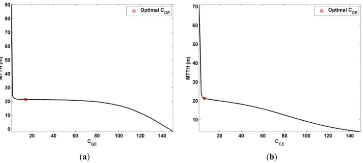
The signal to noise ratio (SNR) of the ULICE system is large enough (with a mean value ~16 within the canopy) to apply a direct threshold approach (Section 3.1) by using Equation (1). After an iterative approach, the optimal values of coefficients CGE and CCE have been derived. In fact, the numbers that

follow the decimal point do not significantly change the final result, so these coefficients have been rounded to be the nearest integers as 13 and 7, respectively. Figure 5 gives the MTTH against the different values of the previous coefficients considered during the iterative approach. The optimal coefficients are located on the flattening part of monotonous decreasing functions.

Figure 5. Mean tree top height (MTTH) against the threshold coefficients CGE (a) and CCE

(b) for the ground echo (GE) and the canopy echo (CE), respectively.

(a) (b)

Using the GE detection alone, a three-dimensional vegetation structure of the forest can be directly derived from the raw lidar profiles corrected from the background sky radiance as shown in Figure 6 for Site 1. Six horizontal planes have been extracted along the vertical to show the apparent treetops of overstory and understory trees, the tree trunks and the ground echoes. The contribution to the lidar return signal between ~5 and 15 m is mainly attributed to trunks and low branches. Two lidar profiles shown on the right of Figure 6 represent the typical signals of overstory and understory trees, respectively.

Several lidar profiles may include information on the same trees. Therefore, Site 1 has been divided into equal pixels (7 m × 7 m) according to the known average distance between trees (~10–15 m) comparatively to the footprint size of ~2 m. Each pixel typically represents one tree, whose canopy height (CH) is retrieved as the highest TTH (HTTH) of all lidar profiles in this pixel. The CH map is shown in Figure 7 where the tallest trees have been identified and located in the sampling area.

Figure 6. Vegetation distributions at Site 1 retrieved from ULICE measurements. The

color code displays the lidar signal amplitude, which indicates the intensities of the inner forest vertical structures. Six planes are defined and highlight the apparent tree tops of overstory and understory trees, the tree trunks and the ground echoes. Two lidar profile examples are shown on the right with opposite x-axes: the blue one is for an understory tree and the red one for an overstory tree.

Figure 7. Lidar-derived canopy height (CH) with pixel size of 7 m × 7 m of Site 1. The

4.1.2. Uncertainties and Validation

The lidar signal has been simulated from real measurements, via a Monte Carlo approach [32], to assess the standard deviation (σTTH_lidar) and the bias (BTTH_lidar) linked to the TTH retrieved from the

lidar profiles. The error calculation has been performed using 64 representative mean lidar profiles that have been simulated. For each profile, 200 random realizations have been considered, ensuring a normal distribution around the mean value. The standard deviation of lidar profile (σL) at the altitude

agl (z) has been calculated from the lidar signal S, the background radiance SBR and the SNR given by:

(14) whereas, in fact, σL(z) = A × (S(z))1/2 is mainly due to shot noise with a constant coefficient A assessed

on the real lidar profile. The SNR values have been retrieved as ~30 for the peaks of both the CE and the GE. The detection procedure was applied to all random realizations to calculate σTTH_lidar and

BTTH_lidar, which were found to be equal to 0.80 m and 0.87 m, respectively. The total uncertainty on

the lidar-derived TTH (εTTH_lidar) is then ~1.2 m, which is reported with other uncertainties in Table 4.

Table 4. Synthesis of uncertainties (ε) and their assessment sources a.

Uncertainty Value Uncertainty Elements Estimate Sources

εTTH_lidar 1.2 m σTTH_lidar = 0.8 m, BTTH_lidar = 0.87 m

Lidar simulation (Monte Carlo)

εTTH_estimate 2.6 m

σTTH_estimate(σTTH_field, σCBH_field) = 0.3 m, with

σTTH_field = 1 m and σCBH_field = 0.02 m

Field measurements

σTTH_estimate(Regression) = 2.6 m Regression fit

εAGCt_field 9%

εAGCt_field(σTTH_estimate, σCBH_field) = 8% Equation (11)

εAGCt_field(σα, σβ, σγ) = 4%

Allometric relationships Equation (11)

εAGC40_field 4% εAGC40_field(εAGCt_field) Simulation

(Monte Carlo)

εQMCH 10%

σQMCH(SNR, Detection) = 10% Lidar measurements

σQMCH(εGPS, εAHRS) = 0.12 m,

with εGPS = 5 m and εAHRS= 3.6 m

Geolocation measurements

εAGC40_lidar 16 tC ha-1

εAGC40_lidar(Regression)= 12 tC ha-1

Regression fit Equation (13),

Figure 8

εAGC40_lidar(εQMCH) = 11% Equation (13)

a _{TTH, tree top height; AGC, aboveground carbon. The detailed descriptions of uncertainties can be found in}

Section 4.

In our experiment, the lidar sampling resolution along the lidar line of sight was settled to be 0.75 m. Through simulation calculations, we found out that there was no significant difference when considering an εTTH_lidar computed for sampling resolutions between 0.3 and 3 m.

) ( ) ( ) ( z S z S z SNR L BR σ − =

Figure 8. Field-derived plot-level AGC estimated for 16 plots of 40 m × 40 m, plotted

against the lidar-derived plot-level QMCH for these plots. The linear regression passing through the points is drawn by a bold line. The uncertainties on the lidar-derived QMCH40 (εQMCH) and field-derived AGC40 (εAGC40_field) are given as error bars. The uncertainty of the

lidar-derived AGC40 (εAGC40_lidar) is drawn as the gray area. The relationships published by

Boudreau et al. [38] and Lefsky et al. [31] are also given.

Lidar measurements of TTHs have been proven in previous works to be in very good agreement with field measurements, using statistical and one-to-one comparisons as shown by Cuesta et al. [6]. In order to validate the lidar-derived tree height attributes, a comparison was conducted in our study over the well-documented central area of Site 1 (Figure 3a). Accordingly, the central area was divided into 5 × 5 plots of 32 m × 32 m in order to be sure that the same highest trees were compared across lidar and field measurements. Such horizontal sampling minimizes the effect of tree growth that mainly occurs for young trees when ground-based and airborne measurements are not coincident in time. For each plot the HTTHs of both lidar and field measurements were identified and assessed on average as 28.5 ± 1.1 m and 28.5 ± 0.6 m, respectively. They are very consistent within an uncertainty of ~1 m, which is similar to the previous results of Cuesta et al. [6].

4.2. AGC Assessment and Related Uncertainties

AGC assessment was conducted over Site 1 (Figure 2), where oaks are the main contributors to the AGC although hornbeams occupy the understory and are the most abundant. This site is divided into 10 × 13 plots of 40 m × 40 m. This surface is equal to the general forest plot size and can be considered as close to the ideal footprints of a spaceborne lidar. The tree characteristics (e.g., TTH, CBH, location) are sufficiently documented in a central area of 2.6 ha (Figure 3a), which is composed of 4 × 4 plots, so as to estimate the AGC from field measurements and calibrate the lidar measurements.

4.2.1. Field-Derived AGC and Related Uncertainties

In the sampling central area of Site 1 (Figure 3a), the CBHs and locations of all trees (1372 trees) in these 16 plots were measured. Amongst these trees, the TTHs were measured on a sub-sample of 134 trees (105 oaks and 29 hornbeams). Thus, the CBH-TTH allometric relationship, as in Equation (8), has been fitted to these field measurements of 105 oaks as shown in Figure 9, with an explained variance of r2 ~ 0.9. The derived values of coefficients µ1, µ2 and µ3 are 30.51 m, 0.27 m cm-1 and 0.92, respectively.

The standard deviations of TTH and CBH from field measurements were calculated from a minimum of six consecutive measurements for each documented oak, and found to be σTTH_field ~ 1 m

and σCBH_field ~ 0.02 m on average. This leads to a mean value of σTTH_estimate(σTTH_field, σCBH_field) ~ 0.3 m

with a negligible bias in the model (Equation 8). The uncertainty of the regression fit on estimated

TTH (σTTH_estimate(Regression)) is ~2.6 m. Thus, the uncertainty on estimated TTH (εTTH_estimate)

is ~2.6 m, as highlighted by the gray area in Figure 9 and listed in Table 4.

The AGC for each documented tree (AGCt) are then assessed by using Equations (9-11), where the

coefficients are adjusted for sessile oaks as follows: α = 0.471 ± 0.014, β = −3.45 × 10−4 ± 0.13 × 10−4 m−1 and γ = 0.377 ± 0.031 m0.5 with a mean residual ε ~0.002 [37]; DEN = 0.55 tg m-3 and

CAR = 0.5 gC g−1 [29]. σTTH_estimate ~ 2.6 m and σCBH_field ~ 20 cm bring an uncertainty on

AGCt (εAGCt_fie1d(σTTH_estimate, σCBH_field), Table 4) of ~8%; whilst the variances (σα, σβ, σγ) of the

coefficients (α, β, γ) bring ~4% uncertainty on AGCt (εAGCt_field(σα, σβ, σγ), Table 4). These values were

computed using a Monte Carlo approach as previously described.

Figure 9. Relationship between the circumference at breast height (CBH) and the tree top

height (TTH) for the 105 oaks in the central area of Site 1. The individual measurements are given by triangles; the standard deviation of the fit linked to the uncertainties on field measurements is given by the gray area.

The field-derived AGCplot has been used rather than AGCt to calibrate the lidar measurements with

the field measurements. As described in Section 3.3, AGCplot can be seen as a statistical summation of

AGCt in the chosen plot surface Splot. The error on field-derived AGCplot for a Splot of 402 m2 (expressed

as εAGC40_field) computed via a Monte Carlo approach is then ~4% (see Table 4), which is shown as

error bars in Figure 8. The estimated AGC derived from field measurements in the central area of Site 1 is then 97 ± 4 tC ha−1.

4.2.2. Lidar-Estimated AGC and Related Uncertainties

The assessment of the lidar-derived AGC passes through the use of Equation (13) and then needs the knowledge of both coefficients a and b. Coefficients a and b are themselves assessed from the lidar-derived QMCH and the field-derived AGCplot of the 16 documented plots of 40 m × 40 m (Figure

8). Hence, we found a = 42.36 and b = 0.24. Such fitting poorly constrains the smaller trees that have not been sampled in Site 1, which is mainly populated with mature oaks (the most relevant for the carbon stock). Nevertheless, the relationships derived from Boudreau et al. [38] and Lefsky et al. [31] surround our curve. The relationship derived from the work of Boudreau et al. [38] is also plotted in Figure 8. It corresponds to a Canadian mixed forest with deciduous and conifer trees with a mean TTH between 4 and 17 m, which are smaller than the oaks of Site 1. The slope of that curve is lower than the one we retrieved. Lefsky et al. [31] also proposed a relationship for a North America deciduous forest as shown in the same figure. Our results are thus in the same range as these previous studies and we will therefore employ the relationship that we have established to perform the uncertainty study.

The uncertainties on the lidar-estimated AGC are generated from two main sources that we will analyze in this section: the retrieval of the QMCH from the full-waveform UV lidar, and the calibration comparatively to the field measurements.

4.2.2.1. Uncertainties on the Lidar-Derived QMCH

In this section, the well-known delta method, using the second-order Taylor expansions to approximate the variance of a function (e.g., [39]), has been applied for the uncertainty calculations. The THP is defined as Equation (2) where each sampling point can be considered to be independent. Therefore, the variance on THPh can be expressed at the second order as follows:

(15) where:

(16)

[

]

1 ) var( 2 _{0 0} 2 0 E E THP E THP E E THP_{h = h + h ⋅ − ⋅ h⋅ h}

[ ]

[ ]





The QMCH can thus be obtained from the THP as given in Equation (7). In order to simplify the calculation of the variance, integration by parts has been applied for the expression of QMCH2 leading to:

= (ln(1 − ) ∙ ℎ )

ℎ ℎ − ln(1 − ) ∙ 2ℎ ∙ ℎ (17)

Across these two parts of the partial integration, the first part is zero by the integration between heights of 0 and TTH. Hence, the approximate variance of QMCH2 _{at the second order can be} retrieved by:

(18) that can be also explained as:

(19) In fact, the uncertainty on QMCH (expressed as σQMCH) for lidar measurements depends on: (1) the

QMCH values; (2) the variances of the lidar signal S(h), which themselves depend on the values of lidar SNR; and (3) the detection of the ground echo and the canopy echo. Through a Monte Carlo approach, σQMCH(SNR) is found to be ~3% for a mean SNR~10 and a QMCH value between 10 and 20 m.

The contributions of the TTH error and detection errors of the GE and the CE have been also assessed. They bring an uncertainty σQMCH(Detection) ~9%. Thus, σQMCH is found to be of the order of 10%.

The uncertainty of laser footprints geolocation also brings an uncertainty on the QMCH, but it appears to be negligible compared with the previous uncertainty sources. Since the accuracy of the GPS (εGPS) and the AHRS (εAHRS) are 5 m and 3.6 m, respectively, the uncertainty of geolocation

is 6.2 m. We assume that the uncertainties along the latitude (λ) and the longitude (φ) are similar, which means σλ = σφ = 4.4 m. As previously, when using a Monte Carlo approach the related standard

deviation of QMCH is found to be σQMCH ~ 0.12 m. It is small because the QMCH here is calculated

from averaged lidar profiles, which reduces the statistical uncertainty and so leads the geolocation uncertainty to be less important.

As a result, the total uncertainty on the lidar-derived plot-level QMCH (εQMCH) is ~10%, whose

uncertainty sources are listed in Table 4. It means there is a QMCH uncertainty of ~1.5 m for the mean QMCH value of ~15 m that is encountered during our experiments.

4.2.2.2. Uncertainties on the Lidar-Derived AGC40

The plot-level AGC for a surface of 40 m × 40 m is expressed as AGC40. The lidar-derived AGC40 is

calculated from the lidar-derived plot-level QMCH following Equation (13). The uncertainty due to this relationship (εAGC40_lidar(Regression)) is found to be close to 12 tC ha−1. εQMCH also contributes to

an error on AGC40 (εAGC40_lidar(εQMCH)) of ~11%. Moreover, at this scale, the errors caused by the lidar

footprint geolocation became negligible compared with the other uncertainty sources. The total





uncertainty on the lidar-derived AGC40 (εAGC40_lidar) is found to be ~16 tC ha−1 (as shown by the gray

area in Figure 8).

A synthesis of uncertainties and their uncertainty sources is given in Table 4. Note that Zolkos et al. [14] discussed the root mean square error (RSE) for different lidars (spaceborne and airborne lidars) and derived from an error model a RSE of between 15 and 40 tC ha−1 for our AGC value.

4.2.2.3. Discussion of the AGC40 and Its Uncertainty

After generalizing the lidar-estimated plot-level AGC (AGC40 in tC ha−1) to the entire sampling area, we found out that the mean AGC40 for 130 plots is 95.5 tC ha−1, with a range from 76 to 123 tC ha−1 and a spatial variability (standard deviation) of ~16 tC ha−1 (shown in Figure 10).

Figure 10. Lidar-derived plot-level aboveground carbon for 40 m × 40 m forest plots

(AGC40) at Site 1.

As shown in Table 5, this result is in a good agreement with the relevant literature studies, among which three approaches have been used: either a modeling method, lidar measurements or field measurements. It demonstrates that our study is based on realistic levels of carbon for deciduous forest. Le Maire et al. [29] found similar results in a Fontainebleau forest region that borders our sampling site. The AGC estimated through their model was about 110 tC ha−1 _{on average, but may reach more} than 200 tC ha−1 in mature oak forests. A similar order of magnitude of the AGC in mature sessile oak forests is also shown by Vallet et al. [40]. Note that the uncertainties are not clearly explained by these authors.

Table 5. AGC synthesis from different references a.

Location Forest type

(tC ha−1)

σAGC

(tC ha−1) Data type References Fontainebleau forest,

France

Deciduous trees

(oak, hornbeam) 96 16 LMe This work

Fontainebleau forest, France

Deciduous trees (oak) 110

- Mo Le Maire et al. [29] Total (oak, fagus, pinus) 88.5

Central France Sessil oak 106 - Mo Vallet et al. [40]

Lopé

National Park, centre Gabon

Tropical rainforest 172.6 48.8 LMe Mitchard et al. [41]

North America

Deciduous forest (oaks, hickories, beechs,

tulip-populars)

118 37.6 LMe Lefsky et al. [31]

Western cascades of Oregon, Pacific Northwest

Young conifer forests 106.5 33.5

FMe Means et al. [17] Mature conifer forests 246 86

North Island, New Zealand

Radiata pine

dominated forests 117 23 LMe Stephens et al. [42] Southeastern Norway,

Norway

Boreal forest 50.6 0.8 LMe

Næsset et al. [43] Spruce, Scots pine 58 1.85 FMe

a _{AGC, aboveground carbon; , the mean AGC; σ}

AGC, the standard deviation of AGC; Mo, modeling

data; LMe, lidar measurements data; FMe, field measurements data.

Zolkos et al. [14] pointed out that lidar is significantly better at estimating carbon than passive optical or radar sensors used alone. Their synthesis of data from about fifty studies, using airborne discrete/full-waveform lidar, indicated a mean residual standard error greater than 10 tC ha−1 for all models. This value ranges from 18% to 34% when it is expressed relative to the average field-measured carbon.

The uncertainties calculated from the field measurements only took into account the coefficients of the allometric law (as α, β and γ). The shape of the law is considered to be exact as defined from field measurements previously published. Nevertheless, it can be an additional important exogenous error source that we cannot quantify in this work.

4.3. Leaf Effect

The effect of leaves on the AGC has been studied over Site 2 (Figure 2). Both in the summer 2012 and in the winter 2013 flight tracks have been realized with footprint size of ~2 m (Figure 3b,c). The choice of flight plan was driven by the wind direction. The useful lidar profile numbers are 35,363 and 58,244, in summer and winter, respectively. After signal processing, the GE and the TTH for each lidar profile have been retrieved. Note that the detections of the GE are not always available for individual lidar profile received in summer, owing to the signal attenuation by canopy leaf strata and the effects of ground cover vegetation.

Following this, the Site 2 was divided into 65 plots of 40 m × 40 m. In each of them the plot-level QMCHs of both summer and winter measurements were retrieved and are represented in Figure 11.

AGC

The relationship appears to be linear. By comparing the QMCHs derived from summer and winter lidar measurements, it seems that the QMCHs in winter (for trees without leaves) have significant smaller values, because the weight of the CE in the total lidar profile is smaller with a large GE. The different structures within the canopy between winter and summer time imply a significant difference of the QMCH with a mean value ~6 m, which leads to an AGC overestimation of ~50% in summer when using winter calibration. As a result, it is necessary to calibrate the relationship (Equation 13) between the lidar-derived QMCH and the field-derived AGC for experiments under different seasons.

However, the AGC estimates do not significantly change between summer and winter. The difference of the lidar signal shapes within the canopy is due to the presence of leaves. The overestimation of AGC could be considered as a non-systematic bias and can be corrected. This possibility is subtended by the results shown in Figure 11. Note that the relative uncertainty on QMCH has been assessed to be similar during winter and summer.

Figure 11. Comparison among the plot-level QMCHs (for 40 m × 40 m forest plots in

Site 2), which are derived from experiments at Site 2 in summer 2012 (with leaf) and winter 2013 (without leaf). The relationship is found to be QMCHwith leaf = 0.996 ×

QMCHwithout leaf + 6.5 (r2 ~0.7).

5. Conclusions

The airborne full-waveform UV (355 nm) lidar demonstrator ULICE has been embedded on an ULA to assess the forest vertical structures, the AGC and the contribution of each related uncertainty source. The accuracy of the vertical location of the canopy structures has been expected to be enhanced by the use of the wavelength of 355 nm because it could minimize the multiple-scattering effect in the canopy. Hence, ULICE should be of interest as a measurement instrument during the preparation of future space missions dedicated to forest studies at the global scale. The experiments have been

conducted over well-documented mid-latitude sites of the Fontainebleau forest in the south-east of Paris. This forest is representative of managed mature deciduous forests of oaks, common in France and in Europe; it provides access to realistic vertical samplings with which to test our canopy-lidar inversion algorithm and the related uncertainties.

A synthesis of the uncertainty sources has been performed. The lidar-derived tree top height (TTH) is obtained with an uncertainty of ~1.2 m. The lidar-derived highest tree top height (HTTH) appears to be in good agreement with the one derived from the field measurements. The lidar-derived quadratic mean canopy height (QMCH), for a plot of 40 m× 40 m compatible with spaceborne measurements, has an uncertainty of ~10%, which depends on the lidar SNR and to a lesser extent on the accuracy of geolocation measurements.

As a demonstration, the AGC has been assessed from the lidar-derived QMCH for forest plots of 40 m × 40 m on the sampling site. Such an assessment allowed us to take into account the main uncertainty sources based on the QMCH (εQMCH), the field measurements (εAGC40_field) and the

calibration between the QMCH and the AGC (εAGC40_lidar), following the recommendations provided by

Zolkos et al. [14] about the lidar measurements applied to forest studies. The AGC of the sampling site has been retrieved as ~95.5 tC ha−1 with a spatial variability of 9 tC ha−1, and an uncertainty of ~16 tC ha−1 (~16%). It is comparable with that of previous independent works operated on the same forest type (e.g., [39]), which shows that our uncertainty study has been conducted for a realistic amount of the AGC. The comparison of lidar measurements between winter and summer enable the assessment of the leaf effect on the AGC. By using the lidar calibration for winter, there is an overestimation of ~50% on AGC estimate in summer. However, a linear relationship has been found between the QMCH retrieved with and without leaves on the same sampling area that offers the capability of using calibration obtained during only one season to retrieve the AGC during the other.

Acknowledgments

The experiment has been funded by the Centre National d’Etudes Spatiales (CNES) and the Commissariat à l’Energie Atomique et aux Energies Alternatives (CEA). We are also grateful for the support offered by the Direction Générale de l'Armement (DGA). Philippe Ciais is acknowledged for his support for the airborne measurements above Fontainebleau. We thank Kamel Soudani and Eric Dufrêne for fruitful discussions. We also express our thanks to Jean-Yves Pontailler and Daniel Berveiller and all those involved in the field inventory data collection and data processing. Fabien Marnas and Julien Totems are also acknowledged for their help during the lidar experiments. We also acknowledge François Dulac, James Ryder and Cecilia Garrec for reviewing the final form of this article.

Author Contributions

Appendix A: Lidar Ground-Track Location (Geolocation)

The geolocation of each footprint is needed because the laser beams were not always emitted with a nadir direction due to slight ULA flight fluctuations. For this calculation, Euler-angles have been introduced where ϕ, θ and ψ are the rotating angles around roll, pitch and yaw axis, respectively (Figure A1).

Figure A1. Representation of three angles (yaw, pitch and roll) between the actual lidar

line of sight and the nadir direction. Both the sensor-fixed coordinate system (Xs, YS, ZS)

and the local tangent plane coordinate system (XG, YG, ZG) are given. The distance d is

defined between the echo (i.e., CE or GE) and the ULA.

On the one hand, the distances represented by the length of the lidar profiles varied slightly according to the emission angle θN between the actual lidar line of sight and the nadir direction. θN

only depends on the roll- and pitch-angle as follows:

(A1) The TTH has to be corrected from the emission angle θN. It is easily calculated from its raw value

(TTHr) by:

(A2) On the other hand, the location of the footprint has been calculated using both the geolocation and the attitude of the ULA. First of all, the measured information recorded by the MTi-G system could be expressed as a vector VS = (0 0 -d) in the Sensor-fixed coordinate system (XS, YS, ZS), where d is the

distance along the line of sight between the target and the ULA (Figure A1). Secondly, a rotation matrix RGS has been introduced so that the vector VS is rotated to be VG = (xG yG zG) (Equation (A3)

and Equation (A4)) in the local tangent plane coordinate system (XG, YG, ZG), which is a Cartesian

) cos (cos cos 1 _{θ φ} θ = − ⋅ N N r TTH TTH = ⋅cos_θ

earth-fixed coordinate system whose X-axis is aligned with the geographic North, Z is defined in the Up direction, and Y is the right handed coordinates (West). As a result, the locations of footprints given by VG could be retrieved by:

(A3)

(A4) Thirdly, by introducing the location of the ULA (Latitude and Longitude measured by the GPS), the locations of footprints could be represented in terms of latitude (λF) and longitude (φF) by:

(20)

where R is the mean Earth radius (R ~6371 km) and z is the ULA altitude above mean sea level (amsl).

Conflicts of Interest

The authors declare no conflict of interest. This is a scientific study using a UV spaceborne demonstrator, which has no commercial goal.

References

1. Anonymous. Climate Change 2013: The Physical Science Basis; Intergovernmental Panel on Climate Change (IPCC): Geneva, Switzerland, 2013; Chapter 6, pp. 465–570.

2. Gibbs, H.K.; Brown, S.; Niles, J.O.; Foley, J.A. Monitoring and estimating tropical forest carbon stocks: Making REDD a reality. Environ. Res. Lett. 2007, 2, 045023.

3. MacArthur, R.H.; MacArthur, J.W. On Bird Species Diversity. Ecology 1961, 42, 594–598.

4. Lefsky, M.A.; Cohen, W.B. Lidar remote sensing of above- ground biomass in three biomes.

Glob. Ecol. Biogeogr. 2002, 11, 393–399.

5. Brown, S.; Pearson, T.; Slaymaker, D.; Ambagis, S.; Moore, N.; Novelo, D.; Sabido, W. Creating a virtual tropical forest from three-dimensional aerial imagery to estimate carbon stocks.

Ecol. Appl. 2005, 15, 1083–1095.

6. Cuesta, J.; Chazette, P.; Allouis, T.; Flamant, P.H.; Durrieu, S.; Sanak, J.; Genau, P.; Guyon, D.; Loustau, D.; Flamant, C. Observing the Forest Canopy with a New Ultra-Violet Compact Airborne Lidar. Sensors 2010, 10, 7386–7403.

7. Allouis, T.; Durrieu, S.; Chazette, P.; Bailly, J.S.; Cuesta, J.; Véga, C.; Flamant, P.; Couteron, P. Potential of an ultraviolet, medium-footprint lidar prototype for retrieving forest structure.

ISPRS J. Photogramm. Remote Sens. 2011, 66, S92–S102.

s T SG S GS G R V R V V = =( )           − − + + − = θ φ θ φ θ ψ φ ψ θ φ ψ φ ψ θ φ ψ θ ψ φ ψ θ φ ψ φ ψ θ φ ψ θ cos cos cos sin sin cos sin sin sin cos cos cos sin sin sin sin cos sin sin cos sin cos sin cos cos sin sin cos cos GS R       + − + = + − = + + − = + + = ) cos( ) ( cos sin sin sin cos ) cos( ) ( sin sin cos sin cos ULA ULA ULA G ULA F ULA G ULA F z R d z R y R z d z R x λ φ ψ ψ θ φ ϕ λ ϕ ϕ ψ φ ψ θ φ λ λ λ

8. Garvin, J.; Bufton, J.; Blair, J.; Harding, D.; Luthcke, S.; Frawley, J.; Rowlands, D. Observations of the earth’s topography from the Shuttle Laser Altimeter (SLA): Laser-pulse echo-recovery measurements of terrestrial surfaces. Phys. Chem. Earth 1998, 23, 1053–1068.

9. Harding, D.J.; Lefsky, M.A.; Parker, G.G.; Blair, J.B. Laser altimeter canopy height profiles methods and validation for closed-canopy, broadleaf forests. Remote Sens. Environ. 2001, 76, 283–297.

10. Brenner, A.C.; Zwally, H.J.; Bentley, C.R.; Csathó, B.M.; Harding, D.J.; Hofton, M.A.; Minster, J.-B.; Roberts, L.; Saba, J.L.; Thomas, R.H.; et al. Derivation of Range and Range Distributions From Laser Pulse Waveform Analysis for Surface Elevations, Roughness, Slope, and Vegetation Heights. In Geoscience Laser Altimeter System (GLAS) Algorithm Theoretical Basis

Document; Version 4.1; Goddard Space Flight Center: Greenbelt, MD, USA, 2003; pp. 1–92.

11. Schutz, B.E.; Zwally, H.J.; Shuman, C.A.; Hancock, D.; DiMarzio, J.P. Overview of the ICESat Mission. Geophys. Res. Lett. 2005, 32, doi:10.1029/2005GL024009.

12. Harding, D.J. ICESat waveform measurements of within-footprint topographic relief and vegetation vertical structure. Geophys. Res. Lett. 2005, 32, doi:10.1029/2005GL023471.

13. Lefsky, M.A.; Harding, D.J.; Keller, M.; Cohen, W.B.; Carabajal, C.C.; Del Bom Espirito-Santo, F.; Hunter, M.O.; de Oliveira, R. Estimates of forest canopy height and aboveground biomass using ICESat. Geophys. Res. Lett. 2005, 32, L22S02.

14. Zolkos, S.G.; Goetz, S.J.; Dubayah, R. A meta-analysis of terrestrial aboveground biomass estimation using lidar remote sensing. Remote Sens. Environ. 2013, 128, 289–298.

15. Wulder, M.A.; White, J.C.; Bater, C.W.; Coops, N.C.; Hopkinson, C.; Chen, G. Lidar plots—A new large-area data collection option: Context, concepts, and case study. Can. J. Remote Sens.

2012, 38, 600–618.

16. Le Toan, T.; Quegan, S.; Davidson, M.W.J.; Balzter, H.; Paillou, P.; Papathanassiou, K.; Plummer, S.; Rocca, F.; Saatchi, S.; Shugart, H.; et al. The BIOMASS mission: Mapping global forest biomass to better understand the terrestrial carbon cycle. Remote Sens. Environ. 2011, 115, 2850–2860.

17. Means, J.E.; Acker, S.A.; Harding, D.J.; Blair, J.B.; Lefsky, M.A.; Cohen, W.B.; Harmon, M.E.; McKee, W.A. Use of large-footprint scanning airborne Lidar to estimate forest stand characteristics in the western cascades of Oregon. Remote Sens. Environ. 1999, 67, 298–308. 18. Grant, R.H.; Heisler, G.M.; Gao, W.; Jenks, M. Ultraviolet leaf reflectance of common urban trees

and the prediction of reflectance from leaf surface characteristics. Agric. For. Meteorol. 2003,

120, 127–139.

19. Ceccaldi, M.; Delanoë, J.; Hogan, R.J.; Pounder, N.L.; Protat, A.; Pelon, J. From CloudSat-CALIPSO to EarthCare: Evolution of the DARDAR cloud classification and its comparison to airborne radar-lidar observations. J. Geophys. Res. Atmos. 2013, 118, 7962–7981. 20. Sugimoto, N.; Nishizawa, T.; Shimizu, A.; Okamoto, H. AEROSOL classification retrieval

algorithms for EarthCARE/ATLID, CALIPSO/CALIOP, and ground-based lidars. In Proceedings of the 2011 IEEE International Geoscience and Remote Sensing Symposium (IGARSS), Vancouver, BC, USA, 24–29 July 2011; pp. 4111–4114.

21. Ansmann, A.; Wandinger, U.; Le Rille, O.; Lajas, D.; Straume, A.G. Particle backscatter and extinction profiling with the spaceborne high-spectral-resolution Doppler lidar ALADIN: Methodology and simulations. Appl. Opt. 2007, 46, 6606–6622.

22. Andersson, E.; Dabas, A.; Endemann, M.; Ingmann, P.; Källén, E.; Offiler, D.; Stoffelen, A.

ADM-AEOLUS: Science Report; Clissold, P., Ed.; ESA Communication Production Office:

Noordwijk, The Netherlands, 2008.

23. Air Création. Available online: http://www.aircreation.fr (accessed on 13 June 2014).

24. Chazette, P.; Sanak, J.; Dulac, F. New approach for aerosol profiling with a lidar onboard an ultralight aircraft: Application to the African Monsoon Multidisciplinary Analysis. Environ. Sci.

Technol. 2007, 41, 8335–8341.

25. Quantel. Available online: http://www.quantel-laser.com/ (accessed on 13 June 2014). 26. National Instruments. Available online: http://france.ni.com/ (accessed on 13 June 2014). 27. Xsens. Available online: http://www.xsens.com/ (accessed on 13 June 2014).

28. ONF. Available online: http://www.onf.fr/ (accessed on 13 June 2014).

29. Le Maire, G.; Davi, H.; Soudani, K.; François, C.; Le Dantec, V.; Dufrêne, E. Modeling annual production and carbon fluxes of a large managed temperate forest using forest inventories, satellite data and field measurements. Tree Physiol. 2005, 25, 859–872.

30. Corif. Available online: http://www.corif.net/site/sitesobs/ (accessed on 13 June 2014).

31. Lefsky, M.A.; Harding, D.; Cohen, W.B.; Parker, G.; Shugart, H.H. Surface lidar remote sensing of basal area and biomass in deciduous forests of eastern Maryland, USA. Remote Sens. Environ.

1999, 67, 83–98.

32. Chazette, P.; Pelon, J.; Mégie, G. Determination by spaceborne backscatter lidar of the structural parameters of atmospheric scattering layers. Appl. Opt. 2001, 40, 3428–3440.

33. Measures, R.M. Laser Remote Sensing: Fundamentals and Applications; Wiley, J., Ed.; Krieger Publishing Company: Malabar, FL, USA, 1984; p. 510.

34. MacArthur, R.H.; Horn, H.S. Foliage Profile by Vertical Measurements. Ecology 1969, 50, 802–804.

35. Brown, S. Measuring carbon in forests: Current status and future challenges. Environ. Pollut.

2002, 116, 363–372.

36. De Dhôte, J.-F.; De Hercé, É. Un modèle hyperbolique pour l’ajustement de faisceaux de courbes hauteur–diamètre. Can. J. For. Res. 1994, 24, 1782–1790.

37. Vallet, P.; Dhôte, J.F.; Moguédec, G.L.; Ravart, M.; Pignard, G. Development of total aboveground volume equations for seven important forest tree species in France. For. Ecol.

Manag. 2006, 229, 98–110.

38. Boudreau, J.; Nelson, R.F.; Margolis, H.A.; Beaudoin, A.; Guindon, L.; Kimes, D.S. Regional aboveground forest biomass using airborne and spaceborne LiDAR in Québec. Remote Sens.

Environ. 2008, 112, 3876–3890.

39. Casella, G.; Berger, R.L. Statistical Inference, 2nd ed.; Duxbury Press: Pacific Grove, CA, USA, 2001; pp. 240–245.

40. Vallet, P.; Meredieu, C.; Seynave, I.; Bélouard, T.; Dhôte, J.F. Species substitution for carbon storage: Sessile oak versus Corsican pine in France as a case study. For. Ecol. Manag. 2009, 257, 1314–1323.

41. Mitchard, E.T.A.; Saatchi, S.S.; White, L.J.T.; Abernethy, K.A.; Jeffery, K.J.; Lewis, S.L.; Collins, M.; Lefsky, M.A.; Leal, M.E.; Woodhouse, I.H.; et al. Mapping tropical forest biomass with radar and spaceborne LiDAR in Lopé National Park, Gabon: Overcoming problems of high biomass and persistent cloud. Biogeosciences 2012, 9, 179–191.

42. Stephens, P.R.; Watt, P.J.; Loubster, D.; Haywood, A.; Kimberley, M.O. Estimation of carbon stocks in New Zealand planted forests using airborne scanning LiDAR. In Proceedings of the ISPRS Workshop on Laser Scanning 2007 and SilviLaser 2007, Espoo, Finland, 12–14 September 2007.

43. Næsset, E.; Gobakken, T.; Solberg, S.; Gregoire, T.G.; Nelson, R.; Ståhl, G.; Weydahl, D. Model-assisted regional forest biomass estimation using LiDAR and InSAR as auxiliary data: A case study from a boreal forest area. Remote Sens. Environ. 2011, 115, 3599–3614.

© 2014 by the authors; licensee MDPI, Basel, Switzerland. This article is an open access article distributed under the terms and conditions of the Creative Commons Attribution license (http://creativecommons.org/licenses/by/3.0/).