Neural-network-based prediction techniques for single station modeling and regional mapping of the <I>fo</I>F2 and M(3000)F2 ionospheric characteristics
11
0
0
Texte intégral
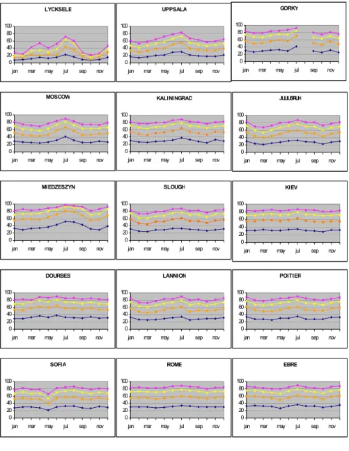
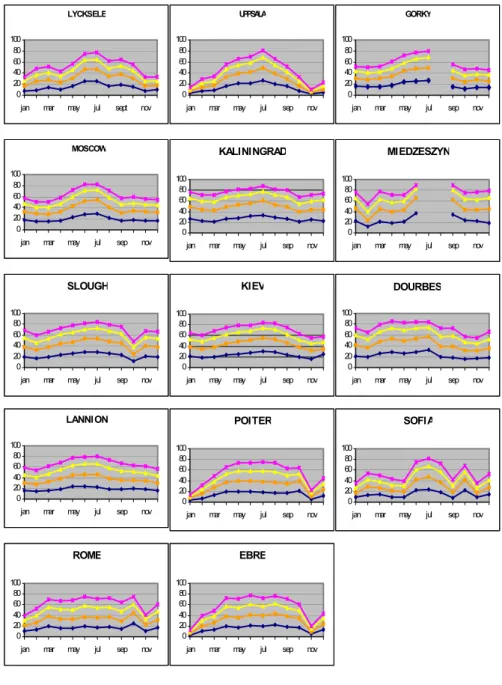
Figure
+5
Documents relatifs