Fisher information matrix for nonlinear mixed effects multiple response models: evaluation of the appropriateness of the first order linearization using a pharmacokinetic/pharmacodynamic model.

HAL Id: inserm-00371363

https://www.hal.inserm.fr/inserm-00371363

Submitted on 27 Mar 2009

HAL is a multi-disciplinary open access archive for the deposit and dissemination of sci-entific research documents, whether they are pub-lished or not. The documents may come from teaching and research institutions in France or abroad, or from public or private research centers.

L’archive ouverte pluridisciplinaire HAL, est destinée au dépôt et à la diffusion de documents scientifiques de niveau recherche, publiés ou non, émanant des établissements d’enseignement et de recherche français ou étrangers, des laboratoires publics ou privés.

Fisher information matrix for nonlinear mixed effects

multiple response models: evaluation of the

appropriateness of the first order linearization using a

pharmacokinetic/pharmacodynamic model.

Caroline Bazzoli, Sylvie Retout, France Mentré

To cite this version:

Caroline Bazzoli, Sylvie Retout, France Mentré. Fisher information matrix for nonlinear mixed effects multiple response models: evaluation of the appropriateness of the first order linearization using a pharmacokinetic/pharmacodynamic model.. Statistics in Medicine, Wiley-Blackwell, 2009, 28 (14), pp.1940-56. �10.1002/sim.3573�. �inserm-00371363�

Fisher information matrix for nonlinear mixed effects multiple response

models: evaluation of the appropriateness of the first order linearization

using a pharmacokinetic/pharmacodynamic model

Caroline Bazzoli*, Sylvie Retout, France Mentré

INSERM, U738, Paris, France; Université Paris Diderot, UFR de Médecine, Paris, France

*

corresponding author:

Caroline Bazzoli,

Inserm U738,

16, rue Henri Huchard

75018 Paris, France

Fax: 33 1 44 85 62 83

SUMMARY

We focus on the Fisher information matrix used for design evaluation and optimization in nonlinear mixed effects multiple response models. We evaluate the appropriateness of its expression computed by linearization as proposed for a single response model. Using a pharmacokinetic–pharmacodynamic (PKPD) example, we first compare the computation of the Fisher information matrix by approximation to one derived from the observed matrix on a large simulation using the stochastic approximation expectation–maximization algorithm (SAEM). The expression of the Fisher information matrix for multiple responses is also evaluated by comparison to empirical information obtained through a replicated simulation study using the first order linearization estimation methods implemented in the NONMEM software (FO, FOCE) and the SAEM algorithm in the MONOLIX software. The predicted errors given by the approximated information matrix are close to those given by the information matrix obtained without linearization using SAEM and to the empirical ones obtained with FOCE and SAEM. The simulation study also illustrates the accuracy of both FOCE and SAEM estimation algorithms when jointly modelling multiple responses and the major limitations of the FO method. This study highlights the appropriateness of the approximated Fisher information matrix for multiple responses, which is implemented in PFIM 3.0, an extension of the R function PFIM dedicated to design evaluation and optimization. It also emphasizes the use of this computing tool for designing population multiple response studies, as for instance in PKPD studies or in PK studies including the modelling of the PK of a drug and its active metabolite.

KEYWORDS: nonlinear mixed effects models; multiple responses; Fisher information matrix; population design; first order approximation; PFIM

1

Introduction

Nonlinear mixed effects models (NLMEM) are widely used to analyze various biological processes described by longitudinal data. Since the primary models developed by Sheiner et

al. [1] in pharmacokinetic (PK) and pharmacodynamic (PD), NLMEM are become widely

used for modelling of biological processes. NLMEM, also called the population approach, allow estimation of the mean value of the parameters in the studied population and their interindividual variability, or population characteristics. NLMEM are also now commonly used for the joint modelling of several biological responses such as the PK of parent drugs and of their active metabolite. NLMEM allow a sparse sampling design with few data points per individual in a large set of individuals. This can be particularly useful in studies in specific populations such as children or patients with serious diseases, where classical studies with a large number of samples are often limited for ethical or physiological reasons.

Estimation of the parameters in NLMEM is commonly performed by maximum likelihood. However, due to the nonlinearity of the regression function, an analytical expression of the log-likelihood in nonlinear mixed effects models cannot be provided. To solve this issue several methods for estimating the parameters have been proposed, based on an approximation of the log-likelihood such as the First Order method (FO) or the First Order Conditional Estimate (FOCE) method proposed by Linsdstrom and Bayes [2]. Both methods use a linearization of the structural model either around the expectation of the random effects parameter (FO) or around individual estimates of the random effects (FOCE). These methods have been implemented in the NONMEM software [3, 4] but also in the nlme function of Splus and R software [5]. Compared to FO, the FOCE method provides less biased estimates and, in the context of joint modelling of multiple responses, is more appropriate with fewer problems of convergence or of inter-individual variance estimation [6, 7]. Alternative methods have also been proposed to maximize the likelihood using a stochastic approximation of the integrals, such as the Gaussian quadrature [8] or the Adaptative Gaussian quadrature methods implemented in the NLMIXED procedure of SAS. Recently, the Stochastic Approximation Expectation–Maximization algorithm (SAEM) has been developed and implemented in the MONOLIX software [9, 10]. It uses a stochastic approximation version of the standard expectation–maximization (EM) algorithm [11, 12]. The convergence and the consistence of the estimates have been proved by the authors. In this algorithm, the EM algorithm is used for finding maximum likelihood estimates of parameters

in models, where the model depends on unobserved variables corresponding to the random effects in the NLMEM.

An appropriate choice of experimental design for estimating parameters in NLMEM is required. Called a population design in this framework, a design is defined as a group of elementary designs; each elementary design is composed of a set of sampling times to be performed in several individuals. Determining a population design involves identifying both the allocation of the sampling times and the whole group structure, that is to say the number of elementary designs, the number of samples per elementary design and the proportion or the number of individuals in each elementary design according to a fixed total number of samples. Simulation studies have shown that the precision of estimation of the parameters depends on the choice of the design [13, 14] and that an appropriate choice can thus substantially improve the efficiency of studies. In the context of NLMEM with sparse designs, the challenge is then to determine the trade-off between few sampling times and informative data to obtain correct parameter estimates.

To evaluate population designs, the theory of optimum experimental design described for instance by Atkinson and Donev [15] or by Walter and Pronzato [16] in classical nonlinear models, has been extended to NLMEM. This theory uses criteria based on the Fisher

information matrix (MF). It comes from the Cramer-Rao inequality; indeed, the inverse of MF

is the lower bound of the variance covariance matrix of any unbiased estimators of the parameters. As the likelihood has no closed form in our framework, a linearization of the model around the expectation of the random effects has been proposed by Mentré et al. [17] and extended by Retout et al. [18] to derive an approximate expression of MF. Accuracy of

this approximation was first shown by simulation of an example based on a real PK study [18, 19], and was confirmed by comparison of the predicted SE computed from this approximate MF to those given by an evaluation of MF without linearization obtained by stochastic

approximation using the SAEM algorithm of MONOLIX [20]. The approximated expression of MF has been implemented in R functions PFIM and PFIMOPT for population design

evaluation and optimization, respectively [21-23]. Recently, PFIM Interface 2.1, a graphical user interface version, has been developed, allowing both evaluation and optimization in the same tool [21]. However, currently, these tools only allow evaluation and optimization of population designs of single response models. For multiple response models, the same linearization method around the expectation of the random effects as for single response models has been proposed to approximate the population MF [24-27]. In those papers,

model of a drug and its metabolite. However, the accuracy of the development of MF by

linearization for multiple responses has not yet been evaluated. Even if the same linearization as in the single response is used, computation can become more complicated for multiple responses. Indeed, some parameters can be included in several responses and the information on those parameters is therefore obtained from each of those response profiles. This is usual in the PKPD context where PD response depends on the PK parameters. Moreover, as noted previously, use of the linearization around the expectation of the random effects appears to be inadequate for joint estimation of multiple response models [6, 7]. The appropriateness of its use in the context of design evaluation is thus also questionable and should be investigated. The objective of this study was therefore to evaluate the first order approximation to compute the Fisher information matrix in NLMEM with multiple responses. To do this, we considered a PKPD simulation example associated with a population design. Then, we compared the predicted standard errors (SE), computed from the approximated expression of MF to those

given by the evaluation of MF without linearization obtained by stochastic approximation

using the SAEM algorithm of MONOLIX. We also performed another evaluation by

comparison of those predicted SE to the empirical ones, obtained by estimation on simulated datasets using three different estimation algorithms: FO and FOCE (with NONMEM); SAEM (with MONOLIX). Based on those simulations, we also compared the performance of those three estimation methods in the same simultaneous analysis of this PKPD model.

In Section 2, we introduce the notations, describe the PKPD example and present the methodology used to evaluate MF and to compare the estimation methods. Section 3 describes

the results of the evaluation and the comparison. Discussion of the results is provided in Section 4. The development of MF for multiple responses is given in detail in the Appendix.

2

Methods

2.1 Notation

In the nonlinear mixed effect multiple response model, an “elementary” design

ξ

_i for one individual i is defined by n sampling times. It is composed of several sub-designs such that _i

(

1, 2, ,

)

i i i iK

ξ = ξ ξ K ξ _{, with}

ik

ξ being the sub-design associated with the kth response, 1, , k= K K_. ik ξ is defined by

(

₁, ₂, ,

)

ik ik ik ikn

t t K t _{, the vector of the} ik

n sampling times for the

observations of the kth response, so that

1 K i ik k n n = =

∑

.

For N individuals, we define a “population design” composed of the N allocated elementary designs

ξ

_i, _i=1,K, _{N . A population design is therefore described by the N elementary} designs for a total number n of observations such that

1 N i i n n = =

_∑

:

{

1, ,

}

Ξ = K N

ξ

ξ

(1)

Usually population designs are composed of a limited number Q of groups of individuals with identical design within each group. Each of these groups is defined by an elementary

designξ_q,q=1,K,Q, which is composed, for the kthresponse, of nqk sampling times

(

tqk1,tqk2, ,tqknqk

)

K _{to be performed in a number}

q

N of individuals. The population design can

then be written as follows:

[

] [

]

{

ξ

1,N1 ;

ξ

2,N2 ; ;

ξ

Q,NQ

}

Ξ = K _{  (2)}

A nonlinear mixed effects multiple response model or a multiple response population model is defined as follows. The vector of observations Y_i for the ith individual is defined as the vector of the K different responses:

1, 1, , T T T T i i i iK Y =_y y K y _{ (3)}

where y ,_ik k=1,K,K _{, is the vector of observations for the k}th _{response. Each of these}

responses is associated with a known function fk which defines the nonlinear structural model. The K functions fk can be grouped in a vector of multiple response models F, such as:

(

) (

)

(

)

1 1 2 2 ( , ) , , , , , , T T T T i i i i i i K i iK F

θ ξ

=_f

θ ξ

f

θ ξ

f

θ ξ

_  K  (4)

where

θ

_i is the vector of all the individual parameters needed for all the response models in

individual i. The vector of individual parameters

θ

i depends on β, the p-vector of the fixed

effects parameters and on b the vector of the p random effects for individual i. The relation _i

between

θ

_i and

(

β

,b_i

)

is modelled by a function g ,

θ

_i =g

(

β

,b_i

)

, which is usually additive, so that

θ β

_i = +b_i, or exponentialso that

θ β

_i = exp

( )

b_i . It is assumed that b_i∼N

(

0,Ω

)

with

Ω defined as a p×p-diagonal matrix, for which, each diagonal element 2 r

ω ,r =1,K,p,

represents the variance of the r component of the vector bth i. The statistical model is thus given by:

(

)

(

, ,

)

i i i i

Y =F g β b ξ +ε (5)

where

ε

_i is the vector composed of the K vectors of residual errors ε_ik, k =1,K,K_,

associated with the K responses. We also suppose ε_ik∼N

(

0,Σ_ik

)

with Σ_ik a n_ik×n_ik-diagonal matrix such that

(

)

(

(

(

)

)

)

2

int int

, , , , , ,

ik

β

bi

σ

erk

σ

slopek

ξ

ik diag

σ

erk

σ

slopekfk g

β

bi

ξ

ik

Σ = + (6)

where σ_{int erk} and

σ

slopek

qualify the model for the variance of the residual error of the

th

k response. The case

σ

_slopek =0 returns a homoscedastic error model, whereas the case

interk 0

σ = returns a constant coefficient of variation error model. The general case where the two parameters differ from 0 is called a combined error model. We then note

(

, , int , ,

)

i

β

bi

σ

er

σ

slope

ξ

i

-diagonal matrix composed of each -diagonal element of Σ_ik with k =1,K,K_. slope

σ and σ_{int er} are two vectors of the K components σ_{int erk} and

σ

slopek

,

k =1,K,K,

respectively. Finally,

conditionally on the value of bi, we assume that the errors

ε

i are independently distributed.

Let Ψ be the vector of population parameters to be estimated such as

2 2 1 int ( , , , , , ) T T T T p er slope

β ω

ω σ

σ

Ψ = K _{and let λ be the vector of variance} terms

λ

T =(

ω

₁2,K,

ω σ

_p2, _interT,

σ

_slopeT)_{, so that} Ψ =T

(

β λT_, T

)

_.

2.2 Population Fisher information matrix for multiple response models

The population Fisher information matrix for a population design Ξ (see Equation (1)), is defined as the sum of the N elementary Fisher information matrices M_F

(

Ψ,

ξ

_i

)

for each individual i:

(

)

(

)

1 , , N F F i i M M ξ = Ψ Ξ =

_∑

Ψ (7)

In the case of a limited number Q of groups, as in Equation (2), it is expressed by:

(

)

(

)

1 , , Q F q F q q M N M

ξ

= Ψ Ξ =

∑

Ψ (8)

The expression of an elementary Fisher information matrix for multiple responses has been extended by Hooker et al. [25] using the same development as for single response models with a first Taylor expansion of the model as in Mentré et al. [17] and Retout et al. [22]. Its expression is given below for one individual i and depends on the approximated marginal expectation E_i and variance V_iof the observationsY_i [28]. Details of this development are given in the Appendix.

(

)

1 1 1 1 , 2 T i i i i F i i m l m l E E V V M Ψ ξ = ∂ V− ∂ + tr V − ∂ V− ∂ 

∂Ψ ∂Ψ  ∂Ψ ∂Ψ  with m and l=1, , dim

( )

Ψ

with, ( )_{i i} ( ( , 0), )_i E Y ≅E =F g

β

ξ

(10)

( )

(

( )

)

(

( )

)

(

int

)

, 0 , , 0 , , 0, , , T i i i i T er slope i F g F g Var Y V b b

β

ξ

β

ξ

β σ

σ

ξ

_∂  _∂  ≅ =  Ω + Σ  _∂   _∂      (11)

This expression has been implemented in an extension of the R function PFIM, PFIM 3.0. This function has been developed for R 2.4.1 and higher versions. The implementation of the population Fisher information matrix assumes that the variance of the observations with respect to the mean parameters is constant (see Appendix). PFIM 3.0 evaluates population designs in NLMEM with multiple responses and thus returns the expected standard errors, defined as the square roots of the diagonal elements of the inverse of MF, on the population

parameters with the design evaluated. To use PFIM 3.0, some prior information has to be supplied by the user such as the structural model, its parameterization and a priori values of the parameters. PFIM 3.0 can also optimize population designs with different optimization options. More details are available in an extensive document that can be freely downloaded with the function PFIM 3.0 on the PFIM website [21].

2.3 PKPD simulation example

In this paper, we use a simple and typical PKPD model as an example to evaluate MF by

simulation. It is derived from the one used by Hooker et al. [25] to illustrate the development of the Fisher information matrix for a multiple response model. The PK model for drug concentration is a one compartment with bolus input and first order elimination given as follows for the sampling time tPK:

exp PK PK PK PK C C dose Cl f (θ , t ) ( t ) V V = − (12)

where θ_PK =

(

Cl V, _C

)

Tis the vector of the PK parameters with Cl and VC, the clearance and the volume in the central compartment, respectively.

The PD model for drug effect is a simple E_max model with baseline, expressed as a function of the predicted concentrations f_PK, and given as follows for the sampling times t_PD :

(

)

max

(

)

0 50 , , , ( , ) PK PK PD PD PK PD PD PK PK PD E f t f t E C f t

θ

θ θ

θ

= + + (13)

where θ_PD =

(

E E₀, _max,C₅₀

)

T is the vector of the PD parameters with E , ₀ E_max andC , the ₅₀

effect at baseline, the maximum effect and the concentration needed to observe half of the maximum effect, respectively.

We assumed an exponential model of the random effects for both the PK and the PD

parameters. We associated a proportional error model with the PK model characterized by the parameter σ_slopePK and a homoscedastic error model with the PD model characterized by the parameter σ_{int erPD}. Thus, the vector of population parameters Ψ is described by the vector of

the fixed effects

(

)

0 max 50

, , , ,

C

T

Cl V E E C

β = β β β β β and by λT the vector composed by the variance of the random effects and by the parameters for the error models such that

(

0 max 50

)

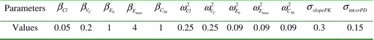
2 2 2 2 2 int , , , , , , C T Cl V E E C slopePK erPD

λ = ω ω ω ω ω σ σ . The dose was fixed to 1 and the parameter values used in this paper are given in Table 1.

We determined a population design associated with this PKPD example. This determination was empirical, without any optimization. The population design was composed of one group of N =100 individuals. They all had 3 sampling times at 0.166, 6 and 12 for PK and 4 sampling times for PD at 0.166, 6, 12 and 20 hours. Therefore, we had one elementary design

(

ξ ξ

_PK, _PD

)

with

ξ

_PK =

(

0.166, 6, 12

)

and

ξ

_PD =

(

0.166, 6, 12, 20

)

. The population design was thus defined by Ξ =

{



(

ξ ξ

PK, PD

)

,N

}

. The curve profiles of the PK and the PD model for the

fixed effects are displayed in Figure 1; the sampling times for each response are overlaid.

2.4 Evaluation of MF for multiple responses

2.4.1 Comparison of MF with and without linearization

In this section, we propose to compare the predicted SE obtained from the approximate MF for

and Samson et al. [29] to show the appropriateness of this approximation in a single response model. This SAEM algorithm allows the observed population Fisher information matrix to be computed according to two approaches. The first approach was developed by Samson et al. [29] and has been used to evaluate an “exact” population Fisher information matrix using the Louis’s principle [30]. It does not require any linearization and can thus be considered as the “true” population Fisher information matrix. The second approach evaluates the Fisher information matrix using a linearization of the model around the conditional expectation of the individual parameters previously estimated by SAEM without any linearization. To perform this comparison, we first computed the predicted MF for the population design

associated with the PKPD example using PFIM 3.0, based on the linearization. We then simulated a dataset of PK and PD observations for 10 000 individuals in order to achieve asymptotic properties using the software R 2.4.1. To do that, we used the parameter values given in Table 1 and the sampling times shown in Figure 1, defining the PKPD example (section 2.3). For each individual i, we simulated a vector of random effects b in _i N

(

0,Ω

)

, where the diagonal elements of Ω are the variance of the random effects, and we calculated the individual parameters using

θ β

i = exp

( )

bi . We then calculated the individual PK

concentrations f_PK(θ_PK, t_PK ) predicted by the model at each time t_PKof

ξ

_PK. We also computed the individual PK concentrations at each time t_PD of

ξ

_PD to derive the concentration fPK

(

θ

PK,tPD

)

for the PD response using Equation (13). PD observations

(

, ,

)

PD PK PD PD

f

θ θ

t were then generated. Finally, for each response, we simulated the random errors

ε

_PK and

ε

_PD from a normal distribution with zero mean and variance derived from Equation (6) using the parameters σ_slopePK andσ_{int erPD}, respectively. Those errors were added to the previously generated PK and PD data to form the simulated observations for the PK and the PD response respectively.

Using MONOLIX (Version 2.1) with SAEM as the estimation algorithm, we estimated the parameters using this simulated dataset and we then derived the observed population Fisher information matrix with the Louis’s principle procedure and the linearization method of SAEM. For these two Fisher information matrices, we then transformed the observed SE for each component of the population vector Ψ obtained with a simulation of N_sim =10000 individuals into predicted SEof a population of N =100 individuals to be adapted to the design of the example using ( ) ( ) /

sim

N i N i sim

For estimation with the SAEM algorithm, we used an initial set of parameters with the values

(

0.2, 0.05, 1.2, 5, 1.5

)

for the fixed effects,

(

1, 1, 1, 1, 0.5

)

for the variance of the random effects

and

(

0.5, 0.5

)

for the residual errors. The default values for the algorithm were used except

for the number of Markov chains, which was set to 4, and the number of iterations with two different steps sizes, which was set to 1000 and 1000 to ensure good convergence.

The predicted SE obtained by linearization with PFIM 3.0 were designated PFIM. The notations SAEM_LO and SAEM_LI denote the predicted SE obtained with the SAEM algorithm using the Louis’s principle and the linearization method, respectively.

2.4.2 Comparison of MF to empirical information through replicated simulation

Another objective was to compare the predicted SE of MF computed from PFIM 3.0 to the

empirical SE obtained by the FO method, the FOCE method and the SAEM algorithm on simulated datasets. To do that, we simulated 1000 datasets of 100 individuals with the software R 2.4.1 using the same PKPD model and population design described previously. Datasets were simulated using a similar method as in section 2.4.1, using the same parameter values and the same sampling times.

For each simulated data file, we estimated the population parameters for the PKPD model using first the FO method and the FOCE with interaction method implemented in NONMEM software version V and then, using the SAEM algorithm in MONOLIX (Version 2.1).

For the estimations using the FO and FOCE methods, two sets of initial parameters were defined. The first corresponded to the value of the parameters used for the simulation (Table 1). The second one was used only in the case of lack of convergence with the first set. The values of the second set of initial parameters were for the fixed effects:

(

0.08, 0.1, 1.5, 3, 0.8

)

; the values of the variance of the random effects and the variance of the residual errors were the same as for the first set of initial parameters. The initial values of the parameters and the different elements required to use the SAEM algorithm were identical to those described in section 2.4.1.

For each parameter of the PKPD model, we compared the predicted SE using the three evaluations of MF with PFIM, SAEM_LO and SAEM_LI,to the empirical SE obtained with

the FO method, the FOCE method and the SAEM algorithm, denoted FO, FOCE, and SAEM, respectively. These empirical SE are defined as the sample estimate of the standard deviation

from the parameter estimates for each method, considering only the subset of datasets fulfilling all convergence conditions.

We were also interested in comparing the distribution of the observed SE provided by each of the estimation methods to the empirical SE and to the predicted SE. In this case, we

considered only the subset of datasets for which both the convergence and the variance– covariance matrix of estimation were obtained. For the distribution of the SE provided by the SAEM algorithm, we considered both methods of computation of the SE, the Louis’s

principle and the linearization.

2.5 Comparison of results for estimation methods with and without linearization

Using the previous simulations, we also compared the three methods of estimation: FO, FOCE and the SAEM algorithm. For each parameter, the relative bias as well as the relative RMSE were computed for the S datasets fulfilling convergence conditions

(

S≤1000

)

, which, for Ψ_l, the lth parameter of the population vector Ψ, are given by:

( )

0 0 1 ˆ 1 S s l l l s l Bias S = _{Ψ − Ψ}  Ψ = _ _ Ψ  

∑

(14)

( )

2 0 0 1 ˆ 1 S s l l l s l RMSE S = _{Ψ − Ψ}  Ψ = _ _ Ψ  

∑

(15)

with Ψˆs_l the estimated value of Ψ_l for the s simulated datasets and th Ψ0_l the true value.

3

Results

3.1 Comparison of MF with and without linearization

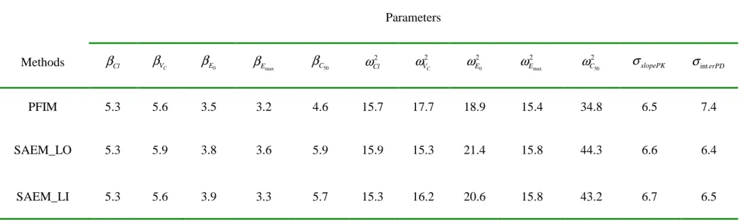
The SE predicted through the use of the SAEM algorithm on a large dataset (SAEM_LI and SAEM_LO) and those predicted by PFIM 3.0 are reported in Table 2 as relative SE, i.e. SE divided by the true value of the parameter, noted RSE and expressed in %. Overall, whatever the method, the RSE of the population parameters were very close for the fixed effects with a difference of at most 1.3% for

50 C

β between the SE predicted by PFIM and the one given by SAEM_LO. Regarding the variance parameters, RSE were also very close, except for

50 2 C

which PFIM seemed to slightly overestimate the parameter estimate precision with a difference of about 10% compared to the SAEM approaches.

This evaluation shows the appropriateness of the extension of the population Fisher Information matrix for multiple response models using the first order approximation.

3.2 Comparison of MF to empirical information through replicated simulation

Convergence was achieved for all datasets and the variance–covariance estimates were obtained for 997 datasets among the 1000 simulated datasets with the FO method.

Convergence with the FOCE method of NONMEM was obtained for only 853 sets. Among those 853 sets, the variance–covariance matrix of estimation was obtained for only 798 sets. Finally, with the SAEM procedure, no problem of convergence or covariance–variance matrix was noted for any of the 1000 datasets.

For each parameter the empirical RSE obtained with the three estimation methods and the predicted RSE of SAEM_LI, SAEM_LO and PFIM are displayed in Figure 2. Concerning the FO method, the empirical RSE were much larger than the RSE of PFIM, SAEM_LI and SAEM_LO except for the PK parameters. This difference is above all important for the PD parameter 2

50

C

ω with a RSE close to 200%. In contrast, the empirical RSE for FOCE and SAEM were very close to the RSE predicted with SAEM_LI, SAEM_LO and PFIM.

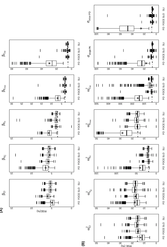
The distribution of observed RSE from the three estimation methods, including both methods of computation of MF with the SAEM algorithm, are reported as boxplots in Figure 3, part (A)

and part (B), for the mean and the variance parameters, respectively. For the FO method, the range of the observed RSE was much larger than for those obtained with the FOCE method or both SAEM procedures. However, the observed RSE of FO were concordant with the

empirical ones. For all the parameters, the RSE predicted with PFIM were consistent with the distribution of the RSE observed with FOCE and the two SAEM procedures but not for FO. The range of the observed RSE for FOCE, SAEM and the corresponding empirical RSE were also concordant. However, for most parameters, the RSE computed using the Louis’s

principle of SAEM had a broader distribution than by using linearization, with values for several datasets being outliers (Figure 3). This problem occurred in particular for the RSE on

50 2 C

ω

parameter.

In this example, the RSE predicted by PFIM, computed by the first order linearization, were thus concordant with the empirical ones and the observed RSE obtained from the simulation

3.3 Comparison of three estimation methods

The relative bias and relative RMSE obtained with the three estimationmethods are presented in Table 3. Convergence was not achieved for 15% of the simulated datasets using the FOCE method whereas the FO method and the SAEM algorithm converged for all datasets.

Regarding the FO method, bias and RMSE were large especially for the parameters of the PD model (fixed effects, random effects and residual errors) whereas FOCE and SAEM provided reasonable bias and RMSE for all the parameters. For the fixed effects, slightly lower bias and RMSE were observed for the SAEM procedure compared to FOCE. We observed important RMSE

(

>40%

)

for the parameter

50 2 C

ω

whatever the estimation method. This is in agreement with the large RSE obtained for that parameter previously.

4

Discussion

We evaluated the expression of the population Fisher information matrix for multiple response models using a linearization of the model [25], as for single response models. Note that our evaluation focused on the case of multiple responses, in which some parameters are involved in several responses. For cases in which parameters differ across responses, the same information would be obtained using MF either for a single response or multiple responses.

The expression of MF for multiple response models has been implemented in PFIM 3.0, an

extension of the R function PFIM, dedicated to population design evaluation and optimization [21-23]. Using a PKPD model, we have shown the appropriateness of the predicted RSE obtained with MF computed by PFIM 3.0 by comparison to those computed without any

linearization by the SAEM algorithm implemented in the MONOLIX software (see Section 3.1). The predicted RSE were indeed all very close except for a slight discrepancy in the RSE for C50 variability.

The simulation study on the PKPD example showed the concordance between the RSE predicted by PFIM and the empirical RSE computed from estimation results with the FOCE or the SAEM algorithm using simulated datasets (see Section 3.2). Regarding results using the FO algorithm, the empirical RSE were much larger than those predicted by PFIM or obtained with FOCE or SAEM, in particular regarding the variability of the PD parameters. The distribution of the RSE obtained with FO, FOCE and SAEM from the simulated data files are in accordance with their respective empirical ones.

Regarding the comparison of the estimation methods for multiple response models, no

problems of convergence were apparent with SAEM or the FO method for the 1000 simulated data files (see Section 3.3). However, it was difficult to fulfill convergence conditions with the FOCE method for which convergence was observed for only 853 of 1000 datasets. The simulation study illustrated the accuracy of the SAEM algorithm in the simultaneous

approach, the parameter estimates being unbiased and with small RMSE. Similar results were observed for the FOCE method, but conclusions must be made with caution due to problems of convergence, as noted previously. Regarding FO, the large bias and RMSE already observed in the context of single response models [31] was also observed in this context of multiple response models with simultaneous estimation. The FO method produced larger RSE on all PD parameters compared to those computed with the FOCE method. This is in

accordance with the recommendation to use the FOCE method instead of the FO method in this simultaneous estimation context [6, 7]. This apparent difference can be explained by considering the difference between FO and FOCE approximations. The FO method

approximates the likelihood by linearizing the population model in its random effects about a value of zero whereas FOCE is defined by a linearization of the model around individual estimates of the random effects. The FOCE method uses more information than the FO method, which is an advantage for estimation in multiple response models. Although the estimation method FO performed badly, the same first order approximation in the computation of MF to predict SE performed well. The limitations of this first order

approximation around the expectation of the random effects thus differ for design evaluation where derivatives of log-likelihood are computed and for parameter estimation.

Several studies have considered the single response, stressing the limitations of this

linearization for design evaluation. Using a simple model with few random effects, Han [32] found that MF was quite different when computed by linearization than by an adaptative

Gaussian quadrature method. Merlé et al. [33] compared the Fisher information matrix computed by linearization to one computed by stochastic simulation and showed that the linearization seems to have no impact on the population D-optimal designs obtained but only on the true efficiency of the designs. Whether via adapative Gaussian quadrature or via stochastic simulation, the evaluation of the Fisher information matrix without linearization is computationally intensive and is also limited to a matrix of small dimensions. Finally, in the context of Bayesian design where prior distributions are used, Han et al. [34] proposed an attractive solution to compute MF; however, it is also time consuming.

Another alternative to the linearization method is to compute the expected Fisher information matrix using the SAEM estimation algorithm, as proposed here. A large dataset is simulated to be close to the asymptotic properties. The observed MF is then estimated for the estimation

performed in this dataset using one of the two methods of deriving MF proposed for SAEM.

This simulation study shows a broader distribution of the observed RSE when MF is

computed by the Louis’s principle [30] compared to the RSE observed with the linearization procedure. Nevertheless, correct results are obtained from both methods. Although the approach using the SAEM algorithm of MONOLIX version 2.1 can be applied for problems with a large number of random effects, it is time consuming (hours) compared to PFIM (seconds). It may be required in specific cases such as when design evaluation is used to predict the power of a test to detect covariates [20]. The appropriateness of the RSEs of PFIM combined with its fast execution emphasizes its advantage in cases of design optimization where a large number of MF often have to be computed. Moreover, in design evaluation and

optimization for nonlinear models, some a priori values of the parameters are required. Often, they are not precisely known, and therefore the need to use exact methods to predict MF is

questionable.

In this study, we empirically determined a population design associated with a simple PKPD example for which the dose was equal to 1. No change in the dose was envisaged because the main purpose of this work was to evaluate MF for a PKPD model associated with one

population design. However, it would be interesting to study the influence of dose on the population design and thus to plan dose optimization in order to have a better understanding of the relationship between the PK and the PD model.

In the present study, we considered only the case of a diagonal Ω matrix with no correlation between the random effects of the PK and the PD parameters. This could be extended by exploring the appropriateness of MF when the PK parameters are directly correlated with the

PD parameters, and thus the development of MF for a full Ω matrix. This development was

performed by Mentré et al. [17] for the correlation of the random effects parameters of single response models and recently by Ogungbenro et al. [26] for multiple response models. Furthermore, the population Fisher information matrix implemented in PFIM 3.0 is

approximated by a block diagonal matrix assuming that the variance of the observations with respect to the mean parameters is constant (see Appendix). It would therefore be interesting to investigate the influence of this assumption on the computation of the Fisher information matrix.

In conclusion, the comparison of RSE predicted by PFIM to RSE computed without any linearization by SAEM as well as to RSE obtained from the simulation study, supports the appropriateness of the approximated Fisher information matrix for multiple response models. Its implementation in PFIM 3.0 provides a useful computing tool for design evaluation and optimization in the development of PKPD or PK studies.

ACKNOWLEDGEMENTS

Part of this work was supported by a grant from F. Hoffmann La Roche Ltd, Basel,

Switzerland. The authors would like to acknowledge Pr Marc Lavielle for his help regarding the use of the MONOLIX software as well as the IFR02 of INSERM and Hervé Le Nagard for the use of the “centre de biomodélisation”.

REFERENCES

1. Sheiner, L.B. and J. Wakefield, Population modelling in drug development. Statistical Methods in Medical Research, 1999. 8(3): p. 183-193.

2. Lindstrom, M.L. and D.M. Bates, Nonlinear mixed effects models for repeated

measures data. Biometrics, 1990. 46(3): p. 673-87.

3. Beal, S.L. and L.B. Sheiner, NONMEM users guide. University of California ed. 1992, San Francisco.

4. Pillai, G.C., F. Mentré, and J.L. Steimer, Non-linear mixed effects modeling - from

methodology and software development to driving implementation in drug

development science. Journal of Pharmacokinetics Pharmacodynamics, 2005. 32(2): p.

161-83.

5. Pinheiro, J.C. and M.D. Bates, Mixed-Effects Models in S and S-Plus. Springer ed. 2000, New-York.

6. Zhang, L., S.L. Beal, and L.B. Sheiner, Simultaneous vs. sequential analysis for

population PK/PD data I: best-case performance. Journal of Pharmacokinetics and

Pharmacodynamics, 2003. 30(6): p. 387-404.

7. Zhang, L., S.L. Beal, and L.B. Sheiner, Simultaneous vs. sequential analysis for

population PK/PD data II: robustness of methods. Journal of Pharmacokinetics and

Pharmacodynamics, 2003. 30(6): p. 405-416.

8. Pinheiro, J.C. and D.M. Bates, Approximations to the log-likelihood function in the

nonlinear mixed effects models. Journal of Computational and Graphical Statistics,

1995. 4: p. 12-35.

9. MONOLIX. 2007: Paris.

10. Samson, A., M. Lavielle, and F. Mentré, Extension of the SAEM algorithm to

left-censored data in nonlinear mixed-effects model: application to HIV dynamics model.

Computational Statistics and Data Analysis, 2006. 51: p. 1562-1574.

11. Delyon, B., M. Lavielle, and E. Moulines, Convergence of a stochastic approximation

version of the EM algorithm. Annals of Statistics, 1999. 27: p. 94-128.

12. Khun, E. and M. Lavielle, Maximum likelihood estimation in nonlinear mixed effects

models. Computational Statistics and Data Analysis, 2005. 49: p. 1020-1038.

13. Al-Banna, M.K., A.W. Kelman, and B. Whiting, Experimental design and efficient

parameter estimation in population pharmacokinetics. Journal of Pharmacokinetics

and Biopharmaceutics, 1990. 18: p. 347-360.

14. Jonsson, E.N., J. Wade, and M.O. Karlsson, Comparison of some practical sampling

strategies for population pharmacokinetics studies. Journal of Pharmacokinetics and

Biopharmaceutics, 1996. 24: p. 245-263.

15. Atkinson, A.C. and A.N. Donev, Optimum Experimental Designs. Clarendon Press ed. 1992, Oxford.

16. Walter, E. and L. Pronzato, Identification of Parametric Models from experimental

Data. Springer ed. 1997, New-York.

17. Mentré, F., A. Mallet, and D. Baccar, Optimal design in random effect regression

models. Biometrika, 1997. 84(2): p. 429-442.

18. Retout, S., F. Mentré, and R. Bruno, Fisher information matrix for non-linear

mixed-effects models: evaluation and application for optimal design of enoxaparin population pharmacokinetics. Statistics in Medicine, 2002. 21(18): p. 2623-39.

19. Retout, S. and F. Mentré, Further developments of the Fisher information matrix in

nonlinear mixed effects models with evaluation in population pharmacokinetics.

20. Retout, S., et al., Design in nonlinear mixed effects models: Optimization using the

Fedorov-Wynn algorithm and power of the Wald test for binary covariates. Statistics

in Medicine, 2007. 26(28): p. 5162-5179. 21. .

22. Retout, S., S. Duffull, and F. Mentré, Development and implementation of the

population Fisher information matrix for the evaluation of population

pharmacokinetic designs. Computer Methods and Programs in Biomedicine, 2001.

65(2): p. 141-51.

23. Retout, S. and F. Mentré, Optimization of individual and population designs using

Splus. Journal of Pharmacokinetics and Pharmacodynamics, 2003. 30(6): p. 417-43.

24. Gueorguieva, I., et al., Optimal design for multivariate response pharmacokinetic

models. Journal of Pharmacokinetics and Pharmacodynamics, 2006. 33(2): p. 97-124.

25. Hooker, A. and P. Vicini, Simultaneous population optimal design for

pharmacokinetic-pharmacodynamic experiments. American Association of

Pharmaceutical Scientists Journal 2005. 7(4): p. 759-785.

26. Ogungbenro, K., et al., Incorporating correlation in interindividual variability for the

optimal design of multiresponse pharmacokinetic experiments. Journal of

Biopharmaceutical Statistics, 2008. 18(2): p. 342-58.

27. Ogungbenro, K., et al., Optimal design for multiresponse

pharmacokinetic-pharmacodynamic models - dealing with unbalanced designs. Journal of

Pharmacokinetics and Pharmacodynamics, 2007. 34(3): p. 313-31.

28. Gagnon, R. and S. Leonov, Optimal population designs for PK models with serial

sampling. Journal of Biopharmaceutical Statistics 2005. 15(1): p. 143-63.

29. Samson, A., M. Lavielle, and F. Mentré, The SAEM algorithm for group comparison

tests in longitudinal data analysis based on non-linear mixed-effects model. Statistics

in Medicine 2007. 26(27): p. 4860-4875.

30. Louis, T.A., Finding the observed information matrix when using the EM algorithm. Journal of the Royal Statistical Society, 1982. 44: p. 226-233.

31. Dartois, C., et al., Evaluation of uncertainty parameters estimated by different

population PK software and methods Journal of Pharmacokinetics and

Pharmacodynamics, 2007. 34(3): p. 289-311.

32. Han, C., Optimal designs for Nonlinear regression Models with Application to HIV

Dynamic Studies. 2002, University of Minnesota: Minneapolis.

33. Merlé, Y. and M. Tod, Impact of pharmacokinetic-pharmacodynamic model

linearization on the accuracy of population information matrix and optimal design.

Journal of Pharmacokinetics and Pharmacodynamics, 2001. 28(4): p. 363-88. 34. Han, C. and K. Chaloner, Bayesian experimental design for nonlinear mixed effects

APPENDIX: Technical details in the development of MF in NLMEM for multiple responses

The population Fisher information matrix M_F

(

Ψ,

ξ

_i

)

for multiple response models for the individual i with design

ξ

_i is given by

(

,

)

2 i

(

; i

)

F i T L Y M Ψ

ξ

=E_−∂ Ψ _ ∂Ψ ∂Ψ   (16)

where L_i

(

Ψ;Y_i

)

is the log likelihood of the vector of observations Y of that individual for the _i

population parameters Ψ. Because F is nonlinear, there is no analytical expression for the log-likelihood L_i

(

Ψ;Y_i

)

, and we use the first-order Taylor expansion of the model

(

_i, _i

)

(

(

, _i

)

, _i

)

F θ ξ =F g β b ξ , around the expectation of b , that is to say around 0: _i

(

)

(

)

( ( , 0), ) , , ( ( , 0), ) T i i i i F g F g b F g b b

β

ξ

β

ξ

≅

β

ξ

+∂  ∂   . (17)

With this approximation, the Equation (5) can be written as:

( ( , 0), ) ( ( , 0), ) T i i i i F g Y F g b b

β

ξ

β

ξ

∂ 

ε

≅ +  + ∂   , (18)

Therefore, the approximated marginal expectation E and variance _i V of _i Y are given by : _i

( )_{i i} ( ( , 0), )_i E Y ≅E =F g β ξ (10)

( )

(

( )

)

(

( )

)

(

int

)

, 0 , , 0 , , 0, , , T i i i i T er slope i F g F g Var Y V b b β ξ β ξ β σ σ ξ _∂  _∂  ≅ =  Ω + Σ  _∂   _∂      (11)

The log-likelihood L is thus approximated by: _i

(

)

( )

( )

(

)

1

(

)

2L_i ;Y_i n_iln 2

π

ln V_i Y_i E_i TV_i− Y_i E_i

− Ψ ≅ + + − − (19)

Note that in this approximation, for sake of simplicity we have assumed that the variance of the error model is not linked to the random effects of the individual but only to the mean parameters. Based on this expression of the log-likelihood L , we can derive the expression of _i

an elementary Fisher information matrix for a multiple response model. For the sake of simplicity, we have omitted the indice i for the individual in the following. MF is a block

matrix depending on the approximated marginal expectation E and variance V of the observations:

(

)

1

(

₍

,

)

_{) (}

(

,

)

₎

, , , 2 F T A E V C E V M C E V B E V

ξ

  Ψ ≅     (20) where 1 1 1 ( ( , )) 2 ( ) T ml m l l m E E V V A E V V tr V V

β

−

β

β

−

β

− ∂ ∂ ∂ ∂ = + ∂ ∂ ∂ ∂ with m and l=1,K,p 1 1 ( ( , ))_ml ( ) m l V V B E V tr V V λ − λ − ∂ ∂ =

∂ ∂ with m and l=1,K, dim

( )

λ

1 1 ( ( , ))_ml ( ) l m V V C E V tr V V λ − β − ∂ ∂ =

∂ ∂ with l=1,K, dim

( )

λ

and m=1,K,p

In this paper, we consider that the variance of the observations with respect to the mean parameters is constant, i.e. ( , )C E V _ml =0.

LIST OF FIGURES

Figure 1. Concentration (left) and effect (middle) profiles versus time for the mean parameter values used in the PKPD example. PK sampling times (left) and PD sampling times (middle) are represented by ●. The right hand graph describes the effect versus concentration.

Figure 2. Barplot of predicted and empirical RSE (%) for the fixed effects, the variances of the random effects and the residual errors of the PKPD example. The empirical RSE

computed by the FO, FOCE methods and the SAEM algorithm on 1000, 853 and 1000 replicates are denoted FO, FOCE and SAEM, respectively. The predicted RSE (%) computed by SAEM and by PFIM are denoted SAEM_LO (for SE obtained by the Louis’s principle), SAEM_LI (for SE obtained by linearization) and PFIM, respectively.

Figure 3. Boxplots of the RSE (%) for fixed effects (A) and for the variance components (B) estimated from 997, 758 and 1000 replicates respectively by the FO, FOCE INTER methods and the SAEM algorithm. SLO denotes the observed RSE of SAEM computed by the Louis’s principle whereas SLI denotes the observed RSE of SAEM computed by linearization. The dotted line represents the RSE predicted by PFIM for each parameter and the star ( )

represents the empirical RSE obtained for each method. Some outliers have been omitted with respect to the Y scale for clarity of the figure.

Table 1. Population parameters values used for the simulated example Parameters

β

Cl βV_C βE₀

β

E_max βC50 2 Cl ω 2 C V

ω

2₀ E

ω

2_max E

ω

2₅₀ C

ω

σslopePK σinterPD

Table 2. Comparison of the relative standard errors (RSE in %) predicted by the SAEM algorithm implemented in MONOLIX V2.1 with both

methods of computation of the SE (noted SAEM_LO for Louis’s principle and SAEM_LI for the linearization method) and predicted by PFIM for the PKPD example.

Parameters Methods

β

Cl βVC βE0

β

Emax βC50 2 Cl ω 2 C V

ω

2₀ E

ω

2_max E

ω

2₅₀ C

ω

σslopePK

σ

interPD

PFIM 5.3 5.6 3.5 3.2 4.6 15.7 17.7 18.9 15.4 34.8 6.5 7.4

SAEM_LO 5.3 5.9 3.8 3.6 5.9 15.9 15.3 21.4 15.8 44.3 6.6 6.4

Table 3. Relative bias (%) and relative RMSE (%) of parameter estimates for datasets with fulfilling convergence conditions (denoted S) using

the FO and the FOCE INTER methods implemented in NONMEM V software and the SAEM algorithm implemented in the MONOLIX V2.1 software. Parameters Methods method S

β

_Cl C V β βE₀ max E

β

βC50 2 Cl ω 2 C V

ω

2₀ E

ω

2_max E

ω

2₅₀ C

ω

σslopePK

σ

interPD

Bias (%) FO 1000 -0.5 0.6 34.5 72.4 131.6 -10.9 -6.9 2.3 -1.7 29.8 -0.3 23.5 FOCE 853 0.3 1.3 1.9 -3.5 -7.3 -0.9 -1.1 -0.5 -0.1 -1.4 1.9 -0.1 SAEM 1000 0.0 -0.1 -0.1 -0.8 0.5 -0.4 -1.0 0.3 -0.1 -0.1 1.3 -0.1 RMSE (%) FO 1000 11.7 7.4 35.1 19.5 135.1 15.9 33.4 48.8 34.5 367.1 26.0 156.8 FOCE _{853 9.2 8.8 4.4 3.4 9.1 15.8 18.1 20.9 16.2 43.5 12.4 27.7} SAEM 1000 5.3 5.6 5.3 3.3 4.0 17.8 16.4 21.7 16.7 41.5 7.8 6.0

Figure 3. βCl FO FOCE S L O S L I 0 5 10 15 RSE(%) (A)

*

*

*

*

βVC FO FOCE S L O S L I 0 5 10 15

*

*

*

*

βE0 FO FOCE S L O S L I 0 5 10 15

*

*

*

*

βEm a x FO FOCE S L O S L I 0 5 10 15 20 25 30

*

*

*

*

βC50 FO FOCE S L O S L I 0 20 40 60 80

*

*

*

*

ωCl 2 FO FOCE S L O S L I 0 10 20 30 40 50 RSE (%) (B)

*

*

*

*

ωVC 2 FO FOCE S L O S L I 0 10 20 30 40 50

*

*

*

*

ωE0 2 FO FOCE S L O S L I 0 50 100 150

*

*

*

*

ωEm a x 2 FO FOCE S L O S L I 0 10 20 30 40 50

*

*

*

*

ωC50 2 FO FOCE S L O S L I 0 100 200 300 400 500

*

*

*

*

σslo pe P K FO FOCE S L O S L I 0 20 40 60 80 100

*

*

*

*

σinte r P D FO FOCE S L O S L I 0 20 40 60 80 100

*

*

*

*