Bayesian models for screening and diagnosis of pulmonary disease

(1)

Bayesian Models for Screening and Diagnosis of

Pulmonary Disease

by

Aneesh Anand

Submitted to the Department of Electrical Engineering and Computer

Science

in partial fulfillment of the requirements for the degree of

Master of Engineering in Electrical Engineering and Computer Science

at the

MASSACHUSETTS INSTITUTE OF TECHNOLOGY

August 2018

c

○ Massachusetts Institute of Technology 2018. All rights reserved.

Author . . . .

Department of Electrical Engineering and Computer Science

August 29, 2018

Certified by . . . .

Richard R. Fletcher

Research Scientist

Thesis Supervisor

Accepted by . . . .

Katrina LaCurts

Chair, Master of Engineering Thesis Committee

(2)

(3)

Bayesian Models for Screening and Diagnosis of Pulmonary

Disease

by

Aneesh Anand

Submitted to the Department of Electrical Engineering and Computer Science on August 29, 2018, in partial fulfillment of the

requirements for the degree of

Master of Engineering in Electrical Engineering and Computer Science

Abstract

Pulmonary and respiratory diseases comprise a large proportion of the global disease burden, responsible for both mortality and disability, with the most common ailments being asthma, chronic obstructive pulmonary disorder (COPD), and allergic rhinitis (AR). This burden is especially concentrated in the developing world, where resources for diagnosing these diseases are more limited. In India, COPD recently became the second leading cause of death. Health workers and many general practitioner doctors are not trained to diagnose pulmonary diseases, leading to high rates of misdiagnosis and underdiagnosis.

Over the past six years, our group has been developing screening tools for pul-monary disease. We have developed a mobile toolkit that consists of an electronic stethoscope, an augmented reality peak flow meter, and an electronic questionnaire. Previously, logistic regression has been used for modeling pulmonary disease. How-ever, logistic regression has certain important limitations: it does not model the problem causally, it isn’t very flexible, and it doesn’t handle missing data well.

In this thesis, we propose a Bayesian framework for disease diagnosis in order to mitigate the issues with logistic regression. A Bayesian network model is presented for predicting the probability of specific pulmonary diseases. The network includes three layers consisting of Diseases, Risk Factors, and Symptoms. We then explored two different approaches to constructing the probability estimates and network parameters employed by the model.

The first approach derived the network parameters using training data from a clinical study conducted at a pulmonary research hospital (Chest Research Founda-tion) located in Pune, India. Arriving patients at the clinic were tested using the MIT mobile toolkit and subsequently examined using a complete pulmonary function testing lab, from which a clinical diagnosis was obtained. Using this data, we built a Bayesian network which was able to accurately detect patients with asthma, COPD, allergic rhinitis, and other pulmonary diseases, with median AUC=0.9 for COPD, AUC=0.92 for Asthma, and AUC=0.89 for Allergic Rhinitis. The Bayesian model was shown to outperform logistic regression in the case of partially missing data.

(4)

In our second approach, we constructed a Bayesian network with probabilities derived from expert opinions. We surveyed experienced pulmonologists and used their responses to parametrize our model. This model was also able to accurately classify patients with asthma, COPD, allergic rhinitis, and other pulmonary diseases. For future deployment in the field, our Bayesian diagnostic model has been inte-grated into Pulmonary Screener, a mobile phone application which is used to collect patient data and calculate probabilities of pulmonary disease. The current work has expanded the previous version of Pulmonary Screener by updating the model struc-ture, improving the workflow, and making the application more intuitive for health professionals.

Given the encouraging results of the generalized Bayesian model presented in this thesis, we believe this framework can be a promising approach for creating diagnostic and screening tools for many applications.

Thesis Supervisor: Richard R. Fletcher Title: Research Scientist

(5)

Acknowledgments

I would like to start by thanking my advisor Rich Fletcher, who constantly guided me and pushed my work forward. Rich has dedicated his work to making a positive impact in the lives of those who need assistance. He has been involved in many projects that work to improve health outcomes through the use of technology. His dedication to service is inspiring and his breadth of knowledge on a variety of subjects both impressed me and helped me refine and focus my research efforts. Rich is a great mentor and researcher, and I am very grateful for the opportunity to work in his group on such an important topic.

I also would like to thank the MIT Tata Center, for its support and guidance. Without the support of the Tata Center, I would not have been able to work on this important area of research. Through the class taught by Chintan Vaishnav and other meetings with the staff, I was able to learn about the broader health landscape in India. The understanding I gained from these conversations helped me focus my work on research that is not only academically meaningful, but useful for the developing world.

I would like to thank the Chest Research Foundation, our partners in Pune, India, who worked with us diligently to successfully conduct clinical studies and provide clinical expertise and guidance. They were fantastic hosts the three times I visited, and each time I left with a renewed vigor and motivation to continue working hard. Dr. Sundeep Salvi is a truly impressive and accomplished physician, who helped me understand the underlying biological mechanisms of pulmonary disease. Yogesh Thorat was very dedicated to the project, and was able to provide expertise from his years working with our group. Finally, I would like to thank Dr. Shrikant Pawar. Not only has he devoted his efforts to successfully conducting the clinical study, he has also displayed an active interest in learning about the algorithmic side of our project and ensuring that we are doing the best possible work we can. Our partners at the Chest Research Foundation give me hope that we can and will solve the health issues facing India and the developing world.

(6)

Finally, I would like to thank my parents. They are both researchers themselves, and they have shown me nothing but love, guidance, and support throughout this process. I could not have made it to this point without them.

(7)

List of Figures

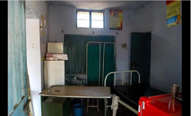
1-1 Rural Clinic in Punjab India . . . 16

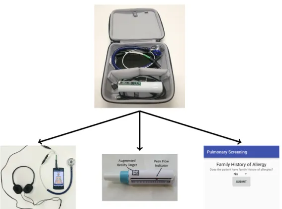
2-1 Mobile diagnostic kit . . . 22

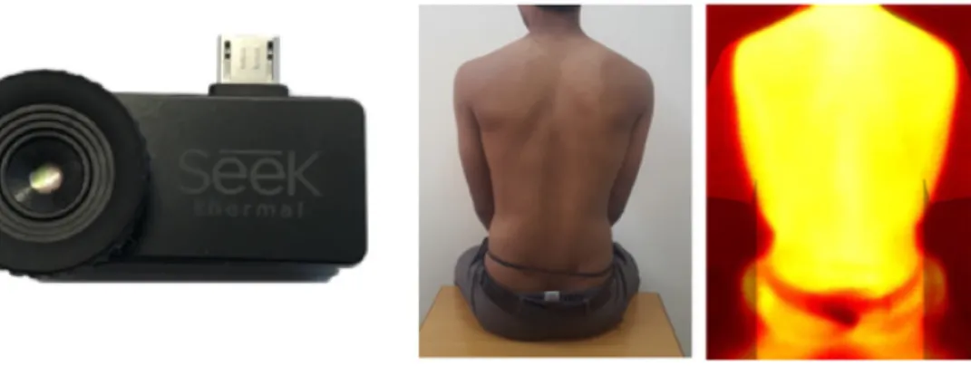
2-2 Thermal Camera . . . 23

2-3 Examples of Mobile Toolkit in use . . . 24

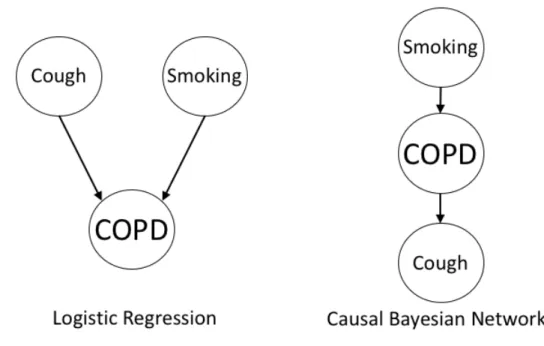
3-1 Graphical models for (left) logistic regression and (right) Bayesian net-work . . . 29

3-2 Graphical model for 3-layer Bayes network for disease diagnosis . . . 32

3-3 Graphical model for generic Bayes net with two layers: features and target variable . . . 35

3-4 Simple Bayesian network with 2 parent nodes and 1 child node . . . . 36

4-1 Full Bayesian network used for disease diagnosis. For clarity, some arrows are omitted. . . 44

4-2 MRC Breathlessness Scale used to grade degree of breathlessness re-lated to activities . . . 48

4-3 Receiver operator curve for data-derived Bayesian network model . . 52

4-4 Model accuracy with different numbers of features removed. Features were removed in order of average logistic regression weight magnitude (highest to lowest). . . 55

5-1 Full expert-derived Bayesian network used for disease diagnosis. For simplicity, some arrows are omitted. . . 65

(12)

5-3 Distribution of survey responses for COPD . . . 69

5-4 Distribution of survey responses for allergic rhinitis . . . 69

5-5 Distribution of survey responses for other pulmonary diseases . . . 70

5-6 Distribution of survey responses for infectious diseases . . . 72

5-7 Receiver operator curve for expert-derived Bayesian network model . 73 6-1 Expert responses for Asthma . . . 80

6-2 Expert responses for COPD . . . 82

6-3 Expert responses for Allergic Rhinitis . . . 82

6-4 Expert responses for Other Pulmonary Diseases . . . 83

6-5 Expert responses for Infectious Diseases . . . 84

7-1 Pulmonary Screener workflow . . . 91

7-2 Screenshots from Pulmonary Screener (current version) . . . 93

7-3 Full diagnostic protocol with branches for infectious, obstructive, al-lergic rhinitis, etc. . . 94

7-4 Diagnostic protocol used by Pulmonary Screener. . . 95

7-5 Distributed system which uses mobile phone clients and a server to make predictions . . . 96

(13)

List of Tables

3.1 Conditional probability table (CPT) for the deterministic OR model . 36

3.2 Conditional probability table (CPT) for the noisy OR model . . . 37

3.3 Conditional probability table (CPT) for the leaky noisy OR model . . 38

4.1 Description of risk factor features . . . 45

4.2 Description of prior probabilities for risk factors . . . 46

4.3 Description of prior probabilities for diseases . . . 47

4.4 Description of symptom features . . . 49

4.5 Disease distribution in the Vodafone study dataset . . . 51

4.6 Classification Results for Logistic Regression . . . 54

4.7 Classification Results for Bayesian Network . . . 54

4.8 Bayesian network confusion matrix from a randomly selected test set 55 4.9 Asthma Entropy . . . 57

4.10 COPD Entropy . . . 58

4.11 AR Entropy . . . 59

4.12 Other Entropy . . . 60

5.1 Survey questions included in pulmonologist questionnaire . . . 67

5.2 Description of prior probabilities for diseases . . . 72

5.3 Classification Results for Expert-Derived Bayesian Network . . . 73

6.1 Classification Results for Data-Derived Bayesian Network . . . 84

(14)

(15)

Chapter 1 Introduction

1.1 Burden of Pulmonary Disease

1.1.1 Global Burden

Pulmonary disease (which includes chronic obstructive pulmonary disease (COPD), asthma, tuberculosis, pneumonia, and lung cancer, among others) is a leading cause of death and disability worldwide. According to the World Health Organization (WHO), 14% of deaths worldwide in 2015 were caused by pulmonary diseases (specifically, COPD, lower respiratory infections, and lung cancers) [1].

Respiratory infections are the leading cause of death in developing countries. 3 million children died from pneumonia and lower respiratory tract infections in 2012, while 1.3 million people died from tuberculosis [2].

235 million people worldwide are estimated to suffer from asthma, and 251 mil-lion people are estimated to suffer from COPD [3] [4]. Asthma is a chronic disease characterized by the narrowing of the airways, causing various levels of breathlessness and wheezing. Asthma patients also often suffer from allergic rhinitis [5].

COPD is an umbrella term used to refer to chronic lung diseases that obstruct airflow in the lungs. COPD is caused by exposure to irritating gases and particulates, often through cigarette smoke and air pollution. COPD symptoms worsen over time, but it can be treated if detected early [5]. The burden of pulmonary disease is

(16)

especially great in developing nations, given an increased prevalence of risk factors like smoking, biomass cooking, and air pollution. 90% of COPD deaths occur in low and middle-income countries [4].

1.1.2 Pulmonary Disease Burden in India

Pulmonary disease is especially prevalent in India due to the risk factors mentioned above. In 2016, COPD grew from the third to the second leading cause of death in India [6]. In India, it is estimated that 20 million people suffer from COPD and 30 million suffer from asthma. Acute respiratory infections have also risen, from 33 million in 2012 to over 40 million in 2016. [7].

(17)

1.2 Pulmonary Disease Diagnosis

1.2.1 Traditional Approach to Diagnosis

The gold standard for pulmonary disease diagnosis includes assessment of symptoms, clinical history, and Pulmonary Function Testing (PFT) [8].

Pulmonary Function Testing consists of:

∙ Spirometry: Patients are asked to blow into a spirometer. Spirometers measure FEV1, the forced expiratory volume of a patient in 1 second, and FVC, the forced vital capacity (total amount exhaled).

∙ Body plethysmography: The patient sits inside an airtight box and inhales and exhales into a breathing tube. Changes in pressure are used to determine the absolute volume of air in the lungs.

∙ Diffusing capacity of the lungs for carbon monoxide (DLCO): This test measures the ability of the lungs to transfer oxygen from the alveoli into the bloodstream. ∙ Impulse oscillometry (optional): Pressure oscillations are applied at the mouth

of a patient to measure the complex frequency response of the lungs.

Tuberculosis is diagnosed through X-ray, skin, sputum, and more recently, ge-netic testing. Lower and upper respiratory tract infections are diagnosed through symptomatic information, cultures, and other lab tests.

In many parts of the developing world, these diagnostic tests are not available to physicians. This is often due to high equipment cost and the need to support specialized technicians [9]. Additionally, medical care in India is out of reach for most. Over 85% in rural areas and 82% of urban residents have no health expenditure support [10].

Thus, tools for the screening and diagnosis of pulmonary disease are generally limited to a clinical history questionnaire and auscultation with a basic stethoscope. In addition, there is a dearth of pulmonologists in most developing countries, so

(18)

diagnoses are often made by general practitioners or other doctors who practice al-ternative forms of medicine (e.g. Ayurveda). Many of these general practitioners are not well-trained to diagnose pulmonary disease, leading to large rates of misdiagnosis and underdiagnosis.

A study indicated that over 50% of COPD patients in India are unaware of their condition [11]. Another multi-center study in India found that over 80% of child asthmatics went undiagnosed [12]. Because asthma and COPD are chronic condi-tions that continually affect quality of life and mortality, this level of underdiagnosis is especially concerning. COPD is a progressive disease, and most of the lung function deterioration occurs in the early stages [11]. Diagnosing COPD patients earlier would allow physicians to intervene and could be the difference between a manageable con-dition and mortality. Early detection of asthma is also important because asthma, if gone untreated, can significantly increase the risk of developing COPD. Though the diseases were once regarded as two separate conditions, asthma and COPD are now often thought to be overlapping conditions [13].

1.2.2 The Need for AI-Based Diagnostic Support

It is clear that there is a severe lack of access to quality care for pulmonary diseases in developing countries. Many of these countries have, in addition to general prac-titioner doctors, community health workers as part of the healthcare system. India has Accredited Social Health Activist (ASHA) workers. While these workers are often not formally trained, they act as a communication mechanism between the healthcare system and rural populations, providing first aid, keeping records, and mobilizing the community [14].

Due to a lack of resources, these workers currently don’t possess tools to help technically screen for diseases. Given the prevalence of smartphones, there is an op-portunity to augment the work of community health workers with mobile applications for disease screening. A diagnostic guidance system could aid inexperienced clinical staff in pulmonary disease diagnosis and could also be integrated with telemedicine systems. In this context, past work in our group has focused on computer-aided

(19)

screening and diagnosis of pulmonary disease with low-cost tools, including a patient questionnaire, mobile stethoscope, and peak flow meter.

1.3 Project Overview

In this project, we sought to build on the efforts of previous researchers in the MIT Mobile Technology Lab [15] [16] to create a screening tool for pulmonary disease. The main contributions of this work are:

∙ A Bayesian network model for screening and diagnosis of pulmonary disease, which achieves high accuracy and is well-suited to handle missing data

∙ Two approaches to parameter estimation for the Bayesian network model: one derived from data collected from lung disease patients, and another derived from the opinions of health professionals. The combination of these approaches allows for a flexible model that is able to provide disease diagnosis even with a low amount of training data

∙ An updated version of the Pulmonary Screener mobile application, built upon the work of Daniel Chamberlain. The updated screening application expands the set of diseases as well as the features included.

The rest of the thesis is organized as follows: Chapter 2 is the Prior Work section. It describes previous work in the MIT Mobile Technology Lab including the MIT Mobile Diagnostic Kit, upon which this work is built. It also discusses other mobile tools, and the remaining challenges in developing a screening tool for pulmonary disease that can be used in the field.

Chapter 3 introduces Bayesian networks as an approach to disease diagnosis. It motivates the need for Bayesian networks due to limitations of other machine learning approaches, details related work on the use of Bayesian networks for disease diagnosis, and describes the principles behind the Noisy OR network.

Chapter 4 describes our approach to constructing a Bayesian network for pul-monary disease diagnosis from training data. It also details the results in terms of

(20)

overall accuracy as well as results with partially missing data. Finally, it contains a sensitivity analysis, which details how specific features contributed to the diagnosis.

Chapter 5 describes our approach to building a Bayesian network from the opinions of experts. It contains analysis of the expert opinion, as well as evaluation of the method’s performance.

Chapter 6 compares the data-derived and expert-derived methods for constructing Bayesian networks. It details the pros and cons of each method, and describes a potential hybrid approach that combines the two.

Chapter 7 describes the mobile implementation of our screening tool, including the model implementation, application workflow, and server implementation. In Chapter 8, we conclude with a discussion.

(21)

Chapter 2 Pulmonary Diagnostic Tools

2.1 Mobile Screening Tools

A variety of academic research groups and start-up companies have developed mobile tools that allow for monitoring of pulmonary health and diagnosis of disease. Most of these tools are various types of electronic stethoscopes for auscultation, and low-cost tools for performing spirometry.

While spirometry is the accepted gold standard for diagnosing obstructive diseases such as COPD and asthma, it is often not used in practice. The challenge of spirom-etry is not the device but rather the administration of the test, which requires a great deal of effort from the patient, and is not viable for children or older patients. As a result, most doctors in developing countries have developed alternative methods of diagnosing COPD and Asthma making use of simpler tools such as peak flow meters or simply questionnaires [17].

DUO is a combined EKG and electronic stethoscope developed by Eko that helps detect cardiac abnormalities [18]. StethoMe uses an electronic stethoscope to diagnose children and send results to a doctor for further analysis [19].

Larson et al. developed SpiroSmart, a low-cost application that performs spirom-etry using the built-in mobile microphone [20]. MySpiroo is a company that has developed a handheld portable spirometer that monitors lung function via a smart-phone application. MIR Smart One is another smartsmart-phone-based spirometer that is

(22)

operated with a mobile application [21]. The Air Smart Spirometer is a portable spirometer that takes measurements with a turbine mechanism and displays the re-sults on a mobile phone [22]. COPD-6 is a mobile tool that serves as a portable spirometer [23].

While these commercial products exist, they are aimed at the developed world, with price points too high to be viable in developing areas. These tools do not address the problem of pulmonary disease screening in low-resource settings.

2.2 MIT Mobile Diagnostic Kit

Figure 2-1: The mobile diagnostic kit. This image does not include the thermal camera, which was recently added to the kit.

The work described in this thesis builds mainly on the efforts of two former MIT students, Daniel Chamberlain and Christian Infante [15] [16]. Daniel Chamberlain

(23)

Figure 2-2: Left: Thermal camera module which connects to a smartphone. Right: The camera in use at the Chest Research Foundation

developed a mobile toolkit, hosted on an Android phone, to screen for COPD and asthma. The kit has three main components:

∙ Questionnaire: With the help of a pulmonologist and questionnaires from past literature, an electronic questionnaire was developed to screen for COPD and asthma. The questionnaire captured basic information (sex, weight, age, etc.), risk factors (alcohol usage, smoking, family history of illness, etc.), as well as the onset, duration, and progress of breathlessness, coughing, nasal symptoms, chest pain, and fever.

∙ Peak Flow Meter: A low-cost portable tool used to determine lung performance. Patients blow quickly into the mouthpiece, which causes a marker to move along a numbered scale. The resulting number is the patient’s peak flow rate, in liters per minute. A mobile application was developed to record multiple trials of the peak flow meter using the phone camera and augmented reality [24].

∙ Electronic stethoscope: A stethoscope was custom-designed to record lung and cough sounds directly onto the Android phone. Lung sounds are recorded from

(24)

11 different sites on the body, while cough sounds are recorded from the trachea. ∙ Thermal camera: A thermal camera was recently added to our toolkit to help diagnose respiratory infections. The compact camera connects to a smartphone and is used to take thermal images of a patient’s chest, side, and back during inhalation and exhalation.

The components of the toolkit are used to generate a set of features. A logistic regression model, trained on a dataset of lung disease patients collected from the Chest Research Foundation, is then used to generate probabilities of each disease based on the set of features collected via the toolkit.

Figure 2-3: Examples of the Mobile Toolkit in use — (left) Mobile questionnaire being conducted. (right) Peak flow meter AR application. This is one of the tools used to collect patient data.

Christian Infante built on this mobile toolkit by adding allergic rhinitis to the list of diseases that the mobile toolkit screens for. Past work showed that the questionnaire and peak flow meter provided the best set of features for distinguishing between these diseases.

2.3 Remaining Challenges

The MIT Mobile Diagnostic kit has been demonstrated to have relatively good perfor-mance as a screening tool for asthma, COPD and allergic rhinitis. However, several

(25)

challenges remain to be addressed in order to create a practical general purpose tool for pulmonary disease screening and diagnosis.

2.3.1 Disease Distribution

One of the challenges facing our diagnostic kit is how to account for the local disease prevalence and incidence, which can vary by country, city, or county. Our diagnostic kit is built with data collected from the Chest Research Foundation. The rates of disease built into our dataset, and therefore our diagnostic toolkit, are a sample skewed by the patients that visit CRF.

We can use respiratory infection to illustrate this point. Respiratory infections such as TB, rhinovirus, pneumonia are the most common pulmonary diseases. They occur more often than asthma and COPD. However, CRF does not see these patients because of protocols that dictate where they can be screened. As a result, our data does not contain any patients with respiratory infection. If our tool was used to screen a patient with a respiratory infection, it would not be able to give the correct diagnosis. Even the diseases that are present in our data occur at different rates than a rural village or an urban slum. In order for the toolkit to be successful, it needs to be able to handle different distributions of disease and still make accurate predictions.

2.3.2 Missing Data

Although research in artificial intelligence and automated diagnostic systems has produced promising results, real-world clinical settings often contain partial or missing data, which severely limits the performance of machine learning models.

Missing data can occur for a variety of reasons:

∙ Quality of patient responses: The data quality of the patient’s responses can be compromised. Patients may not have knowledge of their family medical history of allergies or COPD. Additionally, many subjects lie about sensitive subjects like alcohol and tobacco usage.

(26)

∙ Physiological reasons: It is often difficult for children and the elderly to use peak flow meters, which has rendered PEFR measurements inadequate in past studies [25].

∙ Health worker’s inexperience: Some measurements require training that users may not have. For example, the identification of abnormal lung sounds is not always possible by an unskilled health worker, and this data field is sometimes left blank.

In addition to the reasons listed above, the Indian healthcare system is over-crowded, and thus many health workers and practitioners do not have time to perform extensive testing. Therefore, it is important to be able to adapt and provide accurate diagnoses with a smaller subset of the features.

Due to the challenges of disease distribution and missing data, we chose a Bayesian network modeling approach for this project. In the following sections, we will intro-duce the model, detail our approach, and report results.

(27)

Chapter 3 Bayesian Networks as an Approach to

Diagnosis

3.1 Motivation

The history of diagnostic guidance systems stretches back for decades. A simple diag-nostic guidance system is the clinical algorithm. Clinical algorithms are represented as flowcharts, with each step representing a test to perform or a question to ask the patient. After a series of steps, the algorithm culminates in a diagnosis or treatment option. Clinical algorithms are still in use today- for example, a clinical algorithm can be used to detail how to use spirometry to diagnose asthma or COPD [26].

The main drawbacks of clinical algorithms are that (1) there may be many factors that contribute to a diagnosis that are not easily represented in a flowchart, (2) they are not well-suited to deal with information that is unknown or uncertain, and (3) there is no way to encode nonlinearity of factors that may be linked to each other.

Another approach is expert decision systems, which simplify expert knowledge into a series of rules that can be used to diagnose patients. MYCIN is one such expert system, which used rules to aid the diagnosis of meningitis. However, large sets of rules and the interactions between them were both difficult for domain experts to understand and also often resulted in inaccurate diagnoses [27].

(28)

through their risk factors and the progression of symptoms [28]. Bayesian networks take this approach to disease diagnosis.

There are a variety of criteria that need to be met for a diagnostic guidance system to be successful. Accuracy is chief among these. It is important for a diagnostic model to be able to accurately identify the presence and progression of a patient’s disease. Additionally, it is important that the system is interpretable and able to explain its decisions properly. Interpretability of decisions serves a few purposes: (1) it allows a way to check the reasoning of the system if there are errors, (2) it builds the end users’ (in our case health professionals) trust in the system and thus makes them more likely to use it, and (3) it allows the system to educate users in areas where they may lack knowledge [29]. In our use case, it is also important for the system to be adaptable. What that means is that the system can adapt to situations that may occur in low-resource settings- for example, a shortage of training data or partially missing test data.

3.2 Overview of Bayesian Networks

Bayesian networks are acyclic directed graphs with nodes that represent random variables, and arcs between the nodes that represent the probabilistic dependencies between those variables. If there is a directed arc from variable 𝐴 to variable 𝐵, then 𝐴 is considered to be a parent of 𝐵, and 𝐵 is considered a child of 𝐴. These arcs are more commonly known as edges or links. The probability of a variable is determined by conditional probability tables (CPTs) given the parents of that variable. If a variable has no parents, it is parametrized by a prior probability distribution. The joint probability distribution over all variables in the graph can be decomposed into the prior and conditional distributions of all variables in the graph, as shown in equation (3.1).

(29)

Figure 3-1: Graphical models for (left) logistic regression and (right) Bayesian network

3.3 Comparison to Logistic Regression

In past iterations of our pulmonary screening tool, we’ve used L1-regularized logistic regression as our modeling approach. Logistic regression was chosen for its simplicity, as well as its interpretability. Logistic regression involves learning weights for each feature- those weights can be used as measures of which features are most positively and negatively associated with each disease diagnosis.

However, if we consider logistic regression as a graphical model, we begin to see its limitations. Figure 3-1 shows graphical representations of both logistic regression and a Bayesian network modeling the same variables COPD, cough, and smoking. The nodes in the graph represent random variables and the relationships between variables are represented by the arcs between them.

The logistic regression graph can be thought of as a conditional link 𝑃 (𝐶𝑂𝑃 𝐷|𝐶, 𝑆) between the features Cough (C) and Smoking (S), and the target variable 𝐶𝑂𝑃 𝐷. While the logistic regression treats all variables in the feature set the same, the Bayesian network operates causally. We can see a directed arrow from 𝑆 to 𝐶𝑂𝑃 𝐷 because of the causal association between the two, and the same applies for the arrow

(30)

from 𝐶𝑂𝑃 𝐷 to 𝐶.

The calculation of posterior probabilities utilizes the causal structure of the graph and thus mimics the reasoning of physicians. This allows physicians to more easily understand the structure of the Bayesian network as opposed to the less intuitive logistic function.

3.3.1 Prior Probabilities and Base Rate Neglect

One of the issues with logistic regression is that it fails to properly account for prior probabilities. The Bayesian network allows for more flexibility in setting priors. When constructing a Bayesian network, we can set prior probabilities both for the rates of disease 𝑃 (𝑌 ) and the features 𝑃 (𝑋𝑖). This is especially useful in the context of

diagnosis, where base rates can fluctuate by region and by sample. The rates of smoking, biomass cooking, and asthma are very different across different parts of India, and choosing priors allows us to account for that.

The issue of "base rate neglect" has been studied extensively, and is well-illustrated by this example from Kahneman et al [30].

The probability of breast cancer is 1% for a woman at age 40 who participates in a routine screening. If a woman has breast cancer, the probability is 80 % that she will

have a positive mammography. If a woman does not have breast cancer, the probability is 9.6% that she will also have a positive mammography. A woman in

this age group had a positive mammography in a routine screening. What is the probability that she actually has breast cancer?

Using Bayes’ rule, we can see that the correct answer is

𝑃 (𝑐𝑎𝑛𝑐𝑒𝑟| + 𝑚𝑎𝑚𝑚𝑜𝑔𝑟𝑎𝑚) = 𝑃 (+𝑚𝑎𝑚𝑚𝑜𝑔𝑟𝑎𝑚|𝑐𝑎𝑛𝑐𝑒𝑟) * 𝑃 (𝑐𝑎𝑛𝑐𝑒𝑟)

𝑃 (+𝑚𝑎𝑚𝑚𝑜𝑔𝑟𝑎𝑚) (3.2) = 0.8 * 0.01

0.8 * 0.01 + 0.096 * 0.99 = 0.078 (3.3) Kahneman et al. found that when asked to come up with a probability of cancer for this though experiment, most people greatly overestimated the true value. This is

(31)

because they didn’t fully take into account that the base rate of breast cancer is only 1%. This can be thought of as a biased sample in the mind of the observer. Similarly, biased samples can affect logistic regression.

Suppose that we build a logistic regression model trying to predict the same probability of breast cancer in the example above, using mammogram results as our sole feature. If our sample was biased to contain 50% breast cancer patients and 50% healthy patients, and the positive mammogram rates in each sample remained the same as the example, then the logistic regression model would yield a 75-80% probability of breast cancer for a patient with a positive mammogram. This is a gross overestimate of the 7.8% probability calculated by Bayes’ rule. Because there is no prior probability included to reflect the base rate, the logistic regression estimate is highly inaccurate.

Base rate neglect can also have an effect on our pulmonary disease modeling. As mentioned in the previous chapter, our data was taken from a study conducted at the Chest Research Foundation, where patients with respiratory infections are uncommon. Cough is a symptom that is common in COPD patients as well as patients with the common cold. Because our sample is mainly comprised of COPD patients, the logistic regression will assign a patient with a cough a high probability of having COPD. However, this does not account for the fact that the base rate of COPD is much lower than that of the common cold. If we account for this with prior probabilities (eg. 𝑃 (𝐶𝑂𝑃 𝐷) = 0.05, 𝑃 (𝑐𝑜𝑙𝑑) = 0.3), then the predicted probability of COPD will be more accurate.

3.3.2 Missing Data

Although logistic regression has great value in medical diagnosis because of its sim-plicity and interpretability, one drawback is its inability to deal with missing data. As mentioned in the previous chapter, at the time of prediction on a patient, data can be missing for a variety of reasons. If the logistic regression model is trained on all features in the training set, then there are two main ways to handle missing features at the time of prediction. One method is to conservatively assume that the feature

(32)

value is 0, which zeroes out the associated weight as well. However, that method can result in many false negatives, because the disease probabilities will likely be under-estimated. Another option is to perform some sort of imputation. There are many types of imputation (linear, mean, etc.), but each method adds complication to the modeling process and also comes with its own set of biases.

In contrast, Bayesian networks are well-suited to handle partially missing data. Given the prior and conditional probabilities inherent to the structure of the model, marginalizing over the missing variables yields predictions with reasonably high ac-curacy. A comparison between logistic regression and Bayesian network performance with partially missing data is detailed in Chapter 4.

3.4 A Generalized Bayesian Network for Disease

Di-agnosis

(33)

3.4.1 Network Structure

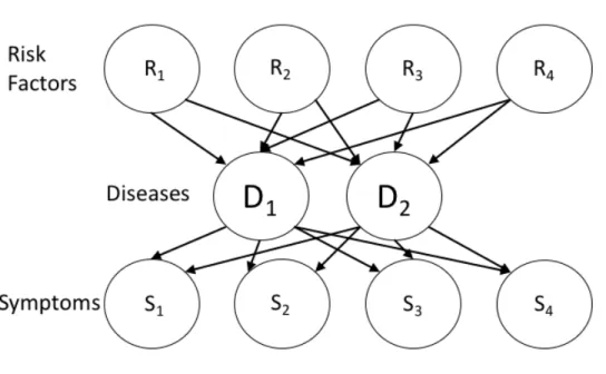
For the purpose of this thesis, we build on the 3-layer model structure used by Pradhan et al. and other researchers in prior work [31]. We represent our model in 3 layers: risk factors, diseases, and symptoms. Risk factors are activities that may put someone at risk of contracting a disease, such as smoking. The disease layer represents the presence or absence of each individual disease. Finally, the symptoms layer contains the features that result from a condition of disease.

Our network structure was developed with the assistance of domain experts from Chest Research Foundation in Pune, India. Figure 3-2 shows a simple Bayesian network with this 3-layer structure.

In order to fully parametrize the model, the following information is required: ∙ Prior probabilities: These probabilities are used to parametrize the variables

in our graph that don’t have parents: risk factors. They are also used to establish the baseline rates of disease. The prior probabilities are derived from population-level studies (described in Chapter 4).

∙ Conditional probabilities: These probabilities determine the strength of the links between different variables in our model. There are various ways to derive the estimates for the conditional probabilities. In the following two chapters, I will discuss two different ways of deriving these unknowns, one based on data and one based on expert opinion.

3.4.2 Past Use of Bayesian Networks for Disease Diagnosis

The use of causal Bayesian networks for medical diagnosis is well-documented [32] [33] [34]. The QMR-DT is one of the earliest models, which formulates diseases and findings in a bipartite graph. There are approximately 600 nodes in the disease layer and 4000 nodes in the finding layer, and the diagnosis problem is to find probabilities of the latent disease variables based on observing a subset of findings. The conditional probabilities that link the two layers were estimated from a combination of disease profile probabilities and hospital discharge data. QMR-DT used a noisy OR model.

(34)

Pradhan et al. extended this two-layer network to three layers by adding a layer of predisposing factors (eg. family history, sex, age) as parents of the disease nodes [31]. Thus, the layers were (1) predisposing factors, (2) diseases, (3) symptoms.

Onisko et al. derived parameters from small data sets as well as expert guid-ance to create a multiple-disorder liver disease diagnostic system (HEPAR-II) using a Bayesian network [35]. Seixas et al. used a 3-layer network, similar to Pradhan, to support the diagnosis of dementia, Alzheimer’s disease, and Mild Cognitive Impair-ment [36].

Anand and Downs used a noisy OR formulation to construct a belief network for asthma case finding. They constructed a two-level network from over 16,000 medical records, using demographic, x-ray, drug, and symptom data for asthma diagnosis [37]. Himes et al. constructed a Bayesian network model to predict COPD from electronic medical records of over 9000 patients [38]. They constructed features from demographic and comorbidity data. Shahmoradi et al. used a noisy OR Bayesian network to classify subtypes of COPD [39].

3.5 The Noisy OR Network

We have described a generalized 3-layer model for disease diagnosis. In this section, we will discuss the noisy OR network, which is a method to reduce the complexity of parameter estimation.

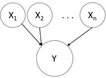
Consider the example in Figure 3-3, where there are 𝑛 parent nodes 𝑋1, 𝑋2, . . . 𝑋𝑛

that feed into one child node 𝑌 . Let us assume that all nodes in the graph represent binary random variables, taking on value 0 or 1. The conditional probability table (CPT) that relates X and 𝑌 has length 2𝑛_{in order to account for the 2}𝑛_{configurations}

of the parent variables X. This CPT grows exponentially with the number of parents of 𝑌 . Thus it becomes difficult to build a CPT for a variable with more than 3 or 4 parents. Additionally, parameters must be chosen for combinations that are not seen in the data. For example, if 𝑌 represents the presence of cough, and X represents a set of diseases (common cold, COPD, asthma, laryngitis, etc.), then the CPT requires

(35)

Figure 3-3: Graphical model for generic Bayes net with two layers: features and target variable

a set of parameters for {𝑎𝑠𝑡ℎ𝑚𝑎, 𝐶𝑂𝑃 𝐷}, {𝑎𝑠𝑡ℎ𝑚𝑎, 𝐶𝑂𝑃 𝐷, 𝑐𝑜𝑚𝑚𝑜𝑛𝑐𝑜𝑙𝑑}, and all other combinations. The complexity of this approach grows with even a small number of variables.

3.5.1 The Deterministic OR Model

The noisy OR network is a method for reducing the complexity of parameter esti-mation in Bayesian networks. It does this by using logic gates to generate full CPTs with a fraction of the number of parameters.

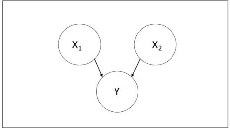
A simplified version of the noisy OR network is a simple OR gate. Figure 3-4 shows a simple network with 2 parents and one child. Table 3.1 demonstrates the calculation of conditional probabilities for the deterministic OR model with 2 parents. This model can be extended to many nodes: if any of 𝑋1, . . . 𝑋𝑛 takes on the value

(36)

Figure 3-4: Simple Bayesian network with 2 parent nodes and 1 child node 𝑃 (𝑦 = 1|𝑥1, 𝑥2) 𝑥1 = 1 𝑥1 = 0

𝑥2 = 1 1 1

𝑥2 = 0 1 0

Table 3.1: Conditional probability table (CPT) for the deterministic OR model

3.5.2 The Noisy OR Model

If we were to consider the previous example of the 𝑋_𝑖′𝑠 as diseases and 𝑌 as cough, then the interpretation of the deterministic OR is that having any one disease will necessarily result in a cough. However, in real life, diseases and symptoms have more uncertainty. To model this uncertainty, we use the noisy OR network [40] [41]. "Noisy" refers to the possibility of a symptom that is not presented (𝑌 = 0) even in the presence of disease(s). We can denote 𝑐𝑖 as the probability that 𝑋𝑖 causes 𝑌

when 𝑋𝑖 = 1 (the link probability) and 𝑞𝑖 = 1 − 𝑐𝑖 as the probability that 𝑌 is not

observed when 𝑋𝑖 = 1 (the failure probability). The noisy OR model is parametrized

by:

𝑃 (𝑦 = 0|x) = Π𝑛_𝑖∈𝐼+_(𝑥)𝑞𝑖 = Π𝑛𝑖∈𝐼+_(𝑥)(1 − 𝑐𝑖) (3.4)

where 𝐼+(𝑥) refers to the set of 𝑋𝑖 variables with value 1. It then follows that:

(37)

These equations imply that 𝑌 is absent when all causes are absent (𝑃 (𝑦 = 1|𝑥1 =

0, 𝑥2 = 0, . . . , 𝑥𝑛 = 0) = 0. It also implies that when only one cause 𝑋𝑖 is present,

then 𝑃 (𝑦 = 1|𝑥𝑖 = 1, ̸ 𝑥𝑖 = 0) = 𝑐𝑖. As the number of causes present increases, the

failure probabilities 𝑞𝑖 associated with each cause 𝑋𝑖 are multiplied, decreasing the

probability of failure and increasing the probability that the cause is present. Table 3.2 shows the CPT for the noisy OR model with 2 parents and 1 child variable. We are able to generate a full CPT for any set of 𝑛 parent nodes with only 𝑛 parameters, the 𝑐𝑖 values. This simplifies the model greatly and allows us to model child variables

with many parents.

𝑃 (𝑦 = 1|𝑥1, 𝑥2) 𝑥1 = 1 𝑥1 = 0

𝑥2 = 1 1 − (1 − 𝑐1)(1 − 𝑐2) 𝑐2

𝑥2 = 0 𝑐1 0

Table 3.2: Conditional probability table (CPT) for the noisy OR model

3.5.3 Leaky Noisy OR

If we were to model how different diseases cause cough, it would be difficult for us to explicitly model every single cause of cough. It would require a large dataset and would also greatly increase the complexity of our model. A simpler method would be to use the leaky noisy OR model.

The leaky noisy OR model includes a leak node 𝑋𝐿 which collectively represents

all other possible causes of 𝑌 that we cannot explicity model. 𝑐𝐿, the leak probability,

is the probability that 𝑌 is present even when all causes that are in our model are absent. This is especially useful in our use case, where a patient may have cough, breathlessness, and nasal symptoms even when they don’t have one of the diseases in our model (asthma, COPD, allergic rhinitis). Similarly, even though a patient may not have engaged in any of the risk factors in our model, they may still contract one of the diseases. In this scenario, we would like to include a leak probability, that represents the baseline probability of each disease.

(38)

to extend the noisy OR model to include leak probabilities.

𝑃 (𝑦 = 1|x) = 1 − 𝑞𝐿(Π𝑛𝑖∈𝐼+_(𝑥)𝑞_𝑖) = 1 − (1 − 𝑐_𝐿)(Π𝑛_𝑖∈𝐼+_(𝑥)(1 − 𝑐_𝑖)) (3.6)

Table 3.3 shows the CPT for the leaky noisy OR model with 2 parents and 1 child. 𝑃 (𝑦 = 1|𝑥1, 𝑥2) 𝑥1 = 1 𝑥1 = 0

𝑥2 = 1 1 − (1 − 𝑐1)(1 − 𝑐2)(1 − 𝑐𝐿) 1 − (1 − 𝑐2)(1 − 𝑐𝐿)

𝑥2 = 0 1 − (1 − 𝑐1)(1 − 𝑐𝐿) 𝑐𝐿

Table 3.3: Conditional probability table (CPT) for the leaky noisy OR model

3.6 The Noisy MAX Network

The models that have been described so far only work for binary variables. However, we often want to use categorical or continuous variables to add finer granularity to our model. For example, we may ask a patient the number of cigarettes that they smoke: this would be considered a continuous variable. If we divided the number of cigarettes smoked into different categories (eg. 0-5 cigarettes, 5-10 cigarettes, over 10 cigarettes), that would be considered a categorical variable. The noisy MAX model is an extension of the noisy OR model to categorical variables.

The noisy MAX requires that 𝑌 is an ordinal variable, which means that it is discrete and ordered. Age is one example of a variable that fits this description.

The link probabilities are given by: 𝑐𝑥𝑖

𝑦 = 𝑃 (𝑍𝑖 = 𝑦|𝑥𝑖) (3.7)

where 𝑍𝑖 represents the value of 𝑌 produced by 𝑋𝑖. Thus if 𝑌 is a discrete

vari-able with 𝑚 unique values, and there are 𝑛 parents of 𝑌 , then there are 𝑛𝑚 link probabilities required for the model.

The cumulative probabilities are given by:

𝑃 (𝑌 ≤ 𝑦|x) = Π𝑖Σ𝑧𝑖≤𝑦𝑐

𝑥𝑖

(39)

Then, the CPT entries can be obtained as follows:

𝑃 (𝑦|x) = 𝑃 (𝑌 ≤ 𝑦|x) − 𝑃 (𝑌 ≤ 𝑦 − 1|x) if 𝑦 ̸= 𝑦𝑚𝑖𝑛 (3.9)

𝑃 (𝑦|x) = 𝑃 (𝑌 ≤ 𝑦|x) if 𝑦 = 𝑦𝑚𝑖𝑛 (3.10)

3.7 Disease Prediction

Once the model structure and parameters are decided, we can use it for disease prediction. Consider using the model in Figure 3-2 to predict disease for an example patient whose data we have collected. This data includes presence and absence of risk factors and symptoms. We want to calculate:

𝑃 (D|R, S) = 𝑃 (R, S|D)𝑃 (D)

𝑃 (R, S) (3.11) where D is the set of diseases, R is the set of risk factors and S is the set of symptoms.

The calculation above, arrived at by Bayes’ Rule, depends on the probabilities 𝑃 (𝑅, 𝑆|𝐷) and 𝑃 (𝐷) in the numerator and the joint probability 𝑃 (𝑅, 𝑆) in the de-nominator. 𝑅 and 𝑆 are conditionally independent given 𝐷, so we can decompose 𝑃 (𝑅, 𝑆|𝐷) into 𝑃 (𝑅|𝐷)𝑃 (𝑆|𝐷). We can use the link probabilities to make this cal-culation, and the priors to make the 𝑃 (𝐷) calculation.

However, the large number of combinations of diseases needed to make the de-nominator calculation make the whole calculation intractable. This issue is well-documented in the Bayesian literature [31] [41]. Instead, we use Markov Chain Monte Carlo, an inference algorithm, to predict disease probabilities.

3.8 Adapting the Model to a Specific Population

We have discussed the benefits that the inclusion of prior probabilities in the Bayesian network offers over logistic regression. There are a variety of approaches that can be

(40)

taken to setting the prior probabilities in order to optimize our model for a given population. If we have information about the rates of disease in the population we are screening, in the form of past studies or expert knowledge, then we can use that to inform our prior probabilities. However, we also do not want to rely too much on a prior estimate and limit the effect to which data can influence the model. Therefore, in this thesis, we have taken the compromise approach of setting ranges of prior probabilities that we have derived from studies of disease rates across India and using cross-validation to select the set of prior probabilities within those ranges that yield the best performance. If we intended to use the Bayesian network model for a screening program in a particular rural community, then we may want to modify our approach. We can change the priors as well as the size of the ranges that we use based on how informed we are about the rates of disease in a particular community.

We can also modify the thresholds we use in order to reflect the prevalence of disease and cost of misclassification. Daniel Chamberlain included in his thesis, a Bayesian cost equation:

𝐸𝐶𝑜𝑠𝑡= 𝐶01𝑝(0|1)𝑝(1) + 𝐶10𝑝(1|0)𝑝(0) (3.12)

where 𝐶01 is the cost of choosing class 0 when class 1 is correct, p(0|1) is the

probability of classifying class 1 as class 0, and p(1) is the prevalence of class 1. We want to minimize the overall cost equation for the population we are screening. We can use the prior estimates to represent the prevalence in the cost equation, and set the costs 𝐶01and 𝐶10according to how much we care about certain misclassifications.

For example, if we are in a population where COPD is severely undiagnosed, we may assign a lower cost to misclassifying a respiratory infection patient as a COPD patient than vice versa. We can then set the thresholds that minimize this equation for our population of interest.

(41)

3.9 Sensitivity Analysis

It is important that the our model’s predictions are interpretable. We, as well as the doctors, need to be able to understand why the model is making certain decisions. In logistic regression, we can do a coefficient analysis and look the weights assigned to each feature to understand which features are important for prediction. In Bayesian networks, we can conduct a sensitivity analysis, which tells us what features contribute to certain predictions. Chapter 4 includes a sensitivity analysis of our Bayesian model.

3.10 Practical Limitations

We can use the noisy MAX network in order to model categorical features. How-ever, this does not account for continous variables, which may be best modeled with aspecific distribution, such as a normal distribution. In order to model continuous variables with a noisy MAX network, we have to bin the variable to convert it into a categorical variable, such as the number of cigarettes example in the previous section. The issue with using continuous probability distributions in the kind of Bayesian network that we have proposed is that it is unclear how to properly generate the entries of the variable’s conditional probability table (CPT).

Consider using a normal distribution to model peak flow rate. We may be able to estimate the mean and standard deviation of peak flow rate for asthma patients, COPD patients, etc. in our training set. However, we need to be able to specify the full CPT of peak flow rate for all combinations of diseases. For example, we need a method to combine the normal distribution for asthma patients 𝑁 (𝜇𝐴, 𝜎𝐴)

with the normal distribution for COPD patients 𝑁 (𝜇𝐶, 𝜎𝐶) for the CPT entry for

{asthma = 1, COPD = 1, AR = 0, Other = 0}. There is no clear way of specifying the CPT entries in these scenarios for continuous distributions. For this reason, it is often necessary to represent such continuous variables in terms of discrete ranges or categories. This simplication enables our Bayesian framework to be applied even to fairly complex diagnostic problems.

(42)

It is important to take these limitations into consideration when evaluating the use of the noisy OR/MAX network. The next chapter describes our approach for deriving the conditional probabilities for the network from data.

(43)

Chapter 4 Data-Derived Bayesian Network

As shown in Chapter 3, it is possible to model disease diagnosis with a 3-layer Bayesian network. We explored two approaches to assigning the link probabilities in the Bayesian network model. The first approach was to derive the parameters from previously collected data, and the second approach was to use expert knowledge to parametrize the model. This chapter details the former approach.

4.1 Design & Implementation

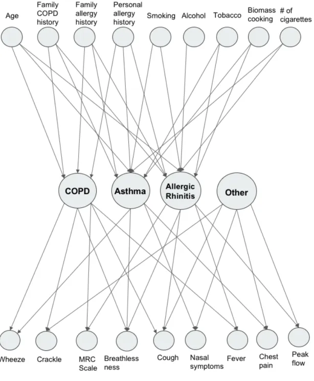
Expanding on the network shown in Figure 3-2, we describe the Bayesian network we use for disease diagnosis, shown in Figure 4-1.

Our Bayesian network structure is represented in three layers: risk factors, dis-eases, and symptoms. Data collected from the CRF study was used to train the network and generate its features. The graphical model developed from these fea-tures is shown in Figure 4-1.

4.1.1 First Layer: Risk Factors

The first layer in the network consists of risk factors. This layer represents the habits or characteristics that can put a patient at risk for a pulmonary disease. These features were taken from responses to the clinical questionnaire. The full set of risk

(44)

Figure 4-1: Full Bayesian network used for disease diagnosis. For clarity, some arrows are omitted.

(45)

factors is detailed in Table 4.1.

Feature Name Feature Description

Age Patient’s age (divided into ranges to create a dis-crete variable: 0-40, 40-60, over 60)

Family History of COPD Does the patient have a family history of COPD? Family History of

Aller-gies

Does the patient have a family history of allergies? Personal History of

Aller-gies

Does the patient have a personal history of aller-gies?

Exposure to Biomass Cooking

Is the patient currently exposed or has the patient been previously exposed to biomass cooking? Smoking History Does the patient currently smoke or has the patient

previously been a smoker?

Tobacco Chewing History Does the patient currently chew tobacco or has the patient previously chewed tobacco?

Number of Cigarettes How many cigarettes does the patient smoke ev-eryday? (divided into ranges to create a discrete variable: 0-5, 5-10, over 10)

Alcohol Consumption History

Does the patient currently consume alcohol or has the patient previously consumed alcohol?

Table 4.1: Description of risk factor features

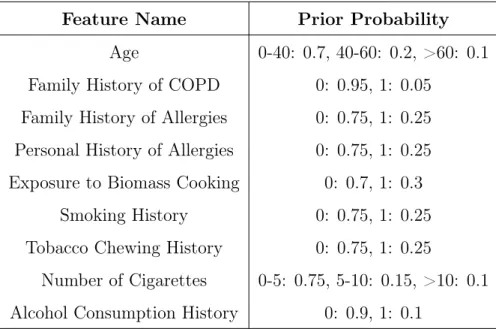
Because these variables do not have parents, we have to encode prior probabilities for all the risk factors in the model. As mentioned in previous chapters, the rates of disease and risk factor presence in our sample are not representative of the population at large. Because of this, we could not use the rates from our dataset as prior probabilities. Instead, we gathered base rates of risk factors from a variety of large-scale population studies in India [42] [43] [44] [45]. The prior probabilities are detailed in Table 4.2.

In addition to the prior probabilities, the model also requires elicitation of the link probabilities 𝑐𝑖 and 𝑐𝑥𝑦𝑖 described in equations 3.4 and 3.7 respectively. Consider

a risk factor as 𝑅 and a disease as 𝐷. The link probability relating the two in the noisy OR model is calculated as:

(46)

Feature Name Prior Probability Age 0-40: 0.7, 40-60: 0.2, >60: 0.1 Family History of COPD 0: 0.95, 1: 0.05

Family History of Allergies 0: 0.75, 1: 0.25 Personal History of Allergies 0: 0.75, 1: 0.25 Exposure to Biomass Cooking 0: 0.7, 1: 0.3

Smoking History 0: 0.75, 1: 0.25 Tobacco Chewing History 0: 0.75, 1: 0.25

Number of Cigarettes 0-5: 0.75, 5-10: 0.15, >10: 0.1 Alcohol Consumption History 0: 0.9, 1: 0.1

Table 4.2: Description of prior probabilities for risk factors. For binary features, 0 means the risk factor is absent (eg. no smoking history), and 1 means it is present (eg. patient has a history of smoking)

𝑐𝑅=

𝑁 (𝑅, 𝐷)

𝑁 (𝑅) (4.1)

Where 𝑁 (𝑅, 𝐷) is the number of patients in the training set with disease 𝐷 and risk factor 𝑅 present and 𝑁 (𝑅) is the number of patients in the training set with risk factor 𝑅 present. Similarly, for 𝑐𝑅𝑖

𝐷 in the noisy MAX model, where 𝑅𝑖 is a specific

discrete state 𝑖: 𝑐𝑅𝑖 𝐷 = 𝑁 (𝑅𝑖, 𝐷) 𝑁 (𝑅𝑖) (4.2)

4.1.2 Second Layer: Diseases

The medical conditions included in layer two are COPD, asthma, allergic rhinitis (AR), and ’Other’ (other pulmonary diseases). All of these diseases are encoded as binary variables, where 0 means the disease is absent and 1 means the disease is present. COPD and asthma are both common pulmonary diseases. Allergic rhinitis is caused by many of the same factors as COPD and asthma- it is often presented as a comorbidity with either asthma or COPD. The ’Other’ category comprises a number

(47)

of pulmonary diseases and conditions. These include URTI, pneumonia, post-TB, and interstitial lung disease (ILD). These diseases can also cause many of the symptoms associated with asthma and COPD. However, they have different pathophysiologies and thus are not triggered by the same risk factors and do not result in the same symptoms. In order to mitigate this issue, there are no links drawn between the risk factors layer and the ’Other’ node: all probabilities are assumed to be 0.

The asthma, COPD, and allergic rhinitis nodes are children of the risk factor variables. However, it is possible that a patient engages in none of the risky behavior and has no family history of illness and still contracts one of these diseases. In this case, it is important to set the leak probabilities 𝑐𝐿 for each of these diseases. The

leak probabilities can be thought of as priors in the sense that they are equivalent to the prior probabilities when all risk factor variables are equal to 0.

We use base rates reported from population-level studies to establish ranges for the leak probabilities [42] [44] [46]. Due to misdiagnosis, underdiagnosis, and differences in rates of disease across India, estimates from population-level studies can vary widely. For example, COPD prevalence estimates have ranged from 3.5% to 6.8% to 16.05% [46]. Because of this, we established ranges for our prior probabilities, and used cross-validation in order to select the values within these ranges that yielded the model with the best performance. The ranges for the disease prior probabilities are summarized in Table 4.3.

Feature Name Prior Probability COPD 0.02 - 0.2 Asthma 0.02 - 0.2 Allergic Rhinitis 0.1 - 0.25 Other 0.05 - 0.2

(48)

4.1.3 Third Layer: Symptoms

The third layer includes symptoms taken from the patient questionnaire as well as peak flow and presence/absence of lung sounds. The full set of symptoms is summa-rized in Table 4.4. The MRC breathlessness scale, one of the symptoms included, was developed by the Medical Research Council to create a numerical grade for severity of breathlessness [47]. The questions used to assess the MRC grade are shown in Table 4-2.

The ’peak flow % of predicted’ feature was derived from the peak flow meter readings. The population predicted value is based on a given patient’s gender, age, and height. The feature included in our model is the patient’s peak flow as percent-age of their population predicted value. The equations used to compute population predicted values are shown in Equations 4.3 and 4.4.

Predicted Male = −1.807 * Age (years) + 3.206 * Height (cm) (4.3)

Predicted Female = −1.454 * Age (years) + 2.368 * Height (cm) (4.4) Because we account for all possible sources of disease by including the ’Other’ category, we do not need prior or leak probabilities for this layer.

Figure 4-2: MRC Breathlessness Scale used to grade degree of breathlessness related to activities

(49)

Feature Name Feature Description

Cough Does the patient have a cough?

Breathlessness Does the patient experience breathlessness?

MRC Scale What is the degree of the patient’s breathlessness? Chest Pain Does the patient experience chest pain?

Fever Does the patient have a fever?

Nasal Symptoms Does the patient have any nasal symptoms?

Peak Flow % of predicted What is the patient’s percentage of predicted peak flow? (divided into ranges to create a discrete vari-able: Greater than 80%, 50-80%, 0-50%)

Wheeze Are there wheezes heard in the patient’s breathing? Crackle Are there crackles heard in the patient’s breathing?

Table 4.4: Description of symptom features

The link probabilities are calculated similarly to the first layer. Consider a disease as 𝐷 and a symptom as 𝑆. The link probability relating the two in the noisy OR model is calculated as:

𝑐𝐷 =

𝑁 (𝑆, 𝐷)

𝑁 (𝐷) (4.5)

For 𝑐𝐷

𝑆𝑖 in the noisy MAX model, where 𝑆𝑖 is a specific discrete state 𝑖:

𝑐𝐷_𝑆_𝑖 = 𝑁 (𝑆𝑖, 𝐷)

𝑁 (𝐷) (4.6)

Link probabilities for the ’Other’ category are calculated in the same way, with ’Other’ being treated as a single disease.

(50)

4.2 Methods

4.2.1 Data Collection & Clinical Study

The data used to train the network was collected as part of a prior study used in the development of the mobile diagnostic toolkit [15]. Data was collected from 325 patients at the Chest Research Foundation in Pune, India. Subjects were selected from an equal sample of all patients arriving at the clinic that exhibited pulmonary symptoms. After excluding some records from training due to low data quality and irrelevant diagnoses, the total subject count came to 309. Table 4.5 shows the distri-bution of diseases in the dataset.

All patients underwent the full suite of tools in the mobile toolkit. First, a tech-nician recorded lung sounds from each patient at eleven different recording locations. A pulmonologist reviewed the recordings and indicated the presence of wheezes or crackles at each location. Each patient took three peak flow meter readings and all values were recorded. A technician administered the patient questionnaire and recorded the responses.

In addition to the mobile toolkit, patients underwent full pulmonary function testing (PFT). This included spirometry, body plethysmography, impulse oscillometry and diffusion tests to determine the final diagnosis. The doctor diagnoses were used as the labels to train our model with.

The protocol for the study received ethics approval from the boards at both CRF (Pune, India) and MIT (Cambridge, MA, USA).

4.2.2 Computational Methods

The Bayesian network model was implemented using the PyMC3 Python library. 80% of the dataset was used as training and 20% was used as a test dataset. The selection was stratified by the disease set so that class sizes were balanced between the training and test sets.

(51)

probabilities. For each cross-validation iteration, the prior probability for each disease was chosen uniformly at random from the ranges described in Table 4.3. Then, the model was evaluated used the mean AUC results from the 3 folds. After 10 iterations, the parameters for the priors that yielded the highest mean AUC were chosen.

These cross-validated parameters were used for test set evaluation. Evaluation was conducted for 10 iterations with randomly selected test sets. The model was conditioned on the risk factors and symptoms of each test record. Then, we ran 1000 MCMC sampling iterations in order to infer the marginal probabilities of each disease. If all disease probabilities were lower than 0.5, the model classified the record as healthy. If both asthma and allergic rhinitis or COPD and allergic rhinitis had disease probabilities higher than 0.5, the patient was classified as having asthma and allergic rhinitis or COPD and allergic rhinitis respectively. Otherwise, the record was classified as the disease category with largest probability.

Diagnosis Count No Pulmonary Disease 98

Asthma only 49 COPD only 36 Allergic Rhinitis only 29 Asthma and Allergic Rhinitis 55 COPD and Allergic Rhinitis 14 Other Pulmonary Disease 28

Total 309

(52)

Figure 4-3: Receiver operator curve for data-derived Bayesian network model

4.3 Results

4.3.1 Prediction Results with Complete Dataset

We compared the Bayesian network model to L1-regularized logistic regression, trained using 3-fold cross-validation with a One vs. Rest classification approach. 10 randomly selected test sets were also used for evaluation of the logistic regression. For both mod-els, we created a receiver-operating-characteristic (ROC) curve. We also calculated sensitivity and specificity and area under the curve (AUC) for each model.

These values were reported at the 25th, median, and 75th percentile.

The results for the logistic regression is shown in Table 4.6 The results for the Bayesian network are shown in Table 4.7. Figure 4-3 also shows the Bayesian network ROC curve for each disease classification for one of the randomly selected test sets. Table 4.8 shows a confusion matrix of the Bayesian network predictions on one of the randomly selected test sets.

(53)

The Bayesian network achieved median AUC values greater than 0.9 for all disease groups except asthma. The network achieved median sensitivity values above 0.9 for all diseases except the ’Other’ category, which had a median sensitivity of 0.55. The specificity values were greater than 0.9 for all disease groups. The low sensitivity for the ’Other’ category makes sense because the category is comprised of patients with a variety of diseases. These diseases have different symptoms and risk factors, and thus there is no strong signal in the link probabilities derived from the data. In other words, it is difficult for the model to learn a set of features that distinctively discerns a patient in the ’Other’ category from patients with asthma, COPD, etc. Thus, the model has low sensitivity in that category.

The confusion matrix makes the misclassifications of the model more clear. Many of the misclassifications come from misclassifying an allergic rhinitis patient as a patient with asthma and allergic rhinitis, or vice versa. Similarly, some COPD pa-tients are classified as having COPD + AR. Additionally, the papa-tients in the ’Other’ category are often misclassified as having asthma.

The Bayesian network had comparable performance to the logistic regression model for all disease groups. The Bayesian model outperformed logistic regression when classifying comorbid asthma and allergic rhinitis, achieving a median AUC of 0.90 compared to the logistic regression’s AUC of 0.72. The Bayesian model also con-sistently achieved higher sensitivity values. The median Bayesian sensitivity values for all diseases except the ’Other’ category were above 0.9. In comparison, the logis-tic regression sensitivity values for asthma, COPD, and allergic rhinitis were close to 0.6, and the sensitivity values for asthma and allergic rhinitis as well as COPD and allergic rhinitis were 0. Both models achieved similar specificity values.

4.3.2 Prediction Results with Partially Missing Data

Bayesian networks can preserve their structure in the case of partially missing data by marginalizing over the missing variables using the prior and conditional probabilities. In contrast, most traditional machine learning models, such as logistic regression, can only be trained on the subset of features that are not missing.

Bayesian models for screening and diagnosis of pulmonary disease

Bayesian Models for Screening and Diagnosis of

Pulmonary Disease

by

Aneesh Anand

Submitted to the Department of Electrical Engineering and Computer

Science

in partial fulfillment of the requirements for the degree of

Master of Engineering in Electrical Engineering and Computer Science

at the

MASSACHUSETTS INSTITUTE OF TECHNOLOGY

August 2018

c

○ Massachusetts Institute of Technology 2018. All rights reserved.

Author . . . .

Department of Electrical Engineering and Computer Science

August 29, 2018

Certified by . . . .

Richard R. Fletcher

Research Scientist

Thesis Supervisor

Accepted by . . . .

Katrina LaCurts

Chair, Master of Engineering Thesis Committee

Bayesian Models for Screening and Diagnosis of Pulmonary

Disease

by

Aneesh Anand

Abstract

Acknowledgments

Contents

List of Figures

List of Tables

Chapter 1

Introduction

1.1

Burden of Pulmonary Disease

1.1.1

Global Burden

1.1.2

Pulmonary Disease Burden in India

1.2

Pulmonary Disease Diagnosis

1.2.1

Traditional Approach to Diagnosis

1.2.2

The Need for AI-Based Diagnostic Support

1.3

Project Overview

Chapter 2

Pulmonary Diagnostic Tools

2.1

Mobile Screening Tools

2.2

MIT Mobile Diagnostic Kit

2.3

Remaining Challenges

2.3.1

Disease Distribution

2.3.2

Missing Data

Chapter 3

Bayesian Networks as an Approach to

Diagnosis

3.1

Motivation

3.2

Overview of Bayesian Networks

3.3

Comparison to Logistic Regression

3.3.1

Prior Probabilities and Base Rate Neglect

3.3.2

Missing Data

3.4

A Generalized Bayesian Network for Disease

Di-agnosis

3.4.1

Network Structure

3.4.2