HAL Id: hal-01578486
https://hal.archives-ouvertes.fr/hal-01578486
Submitted on 29 Aug 2017HAL is a multi-disciplinary open access archive for the deposit and dissemination of sci-entific research documents, whether they are pub-lished or not. The documents may come from teaching and research institutions in France or abroad, or from public or private research centers.
L’archive ouverte pluridisciplinaire HAL, est destinée au dépôt et à la diffusion de documents scientifiques de niveau recherche, publiés ou non, émanant des établissements d’enseignement et de recherche français ou étrangers, des laboratoires publics ou privés.
An accurate algorithm for evaluating rational functions
Stef Graillat
To cite this version:
Stef Graillat. An accurate algorithm for evaluating rational functions. Applied Mathematics and Computation, Elsevier, 2018, 337, pp.494-503. �10.1016/j.amc.2018.05.039�. �hal-01578486�
An accurate algorithm for evaluating rational functions
Stef Graillat
*August 29, 2017
Abstract
Several different techniques intend to improve the accuracy of results computed in floating-point precision. Here, we focus on a method to improve the accuracy of the evaluation of rational functions. We present a compensated algorithm to evaluate rational functions. This algorithm is accurate and fast. The accuracy of the computed result is similar to the one given by the classical algorithm computed in twice the working precision and then rounded to the current working precision. This algorithm runs much more faster than existing implementation producing the same output accuracy.
Keywords: floating-point, error-free transformation, rational function, Horner scheme, accuracy, rounding
errors
AMS Subject Classifications: 15-04, 65G99, 65-04
1 Introduction
Evaluating a polynomial or a rational function is ubiquitous in computational sciences and their applications. For example, in signal processing, transfer functions are very often rational functions. Moreover, real functions are often approximated by polynomials or rational functions.
In this paper, we present fast and accurate algorithms to compute the evaluation of a rational function. Our aim is to increase the accuracy at a fixed precision. We show that the results have the same error estimates as if computed in twice the working precision and then rounded to working precision. This paper was motivated by papers [14,7,6], where similar approaches are used to compute summation, dot product, and polynomial evaluation.
This outline of this article is as follows. In Section2, we quickly recall some information on floating-point arithmetic and we give some definitions and notations used in the sequel. In Section3, we recall the com-pensated Horner scheme [7,6]. This algorithm makes it possible to evaluate a polynomial whose accuracy of the computed result is similar to the one given by the classical algorithm computed in twice the working precision and then rounded to the current working precision. Section4is devoted to the study of the accuracy of the classic algorithm to evaluate a rational function with Horner scheme. We also define and compute
*Sorbonne Universit´es, UPMC Univ Paris 06, CNRS, UMR 7606, LIP6, F-75005 Paris, France ([email protected],http://www-pequan.lip6.fr/~graillat).
a closed formula for the condition number of rational function evaluation. A compensated algorithm for evaluating rational functions is presented in Section5. This algorithm evaluates a fractional function and gives an accuracy of the computed result that is similar to the one given by the classical algorithm computed in twice the working precision and then rounded to the current working precision. Finally, numerical experiments showing the accuracy and the performance of our new compensated algorithm to evaluate fractional functions are presented in Section6.
2 Floating-point arithmetic
Throughout the paper, we assume to work with a floating-point arithmetic adhering to IEEE 754 floating-point standard [9]. We assume that no overflow nor underflow occur. The set of floating-point numbers is denoted by F, the relative rounding error by u. For IEEE 754 double precision, we have u = 2−53and for single precision
u = 2−24.
We denote by fl(⋅) the result of a floating-point computation, where all operations inside parentheses are done in floating-point working precision. Floating-point operations in IEEE 754 satisfy [8]
fl(a ○ b) = (a ○ b)(1 + ε1) = (a ○ b)/(1 + ε2) for ○ = {+, −, ⋅, /} and ∣εν∣ ≤ u.
This implies that
∣a ○ b − fl(a ○ b)∣ ≤ u∣a ○ b∣ and ∣a ○ b − fl(a ○ b)∣ ≤ u∣ fl(a ○ b)∣ for ○ = {+, −, ⋅, /}. (2.1) We use standard notation for error estimations. The quantities γnare defined as usual [8] by
γn ∶=
nu
1 − nu for n ∈ N, where we implicitly assume that nu ≤ 1.
Following [8], we also use the following classic properties in error analysis (we always assume that nu < 1): γk< γk+1and (1 + u)γk≤ γk+1.
One can notice that a ○ b ∈ R and a ⊚ b ∶= fl(a ○ b) ∈ F but in general we do not have a ○ b ∈ F. It is known that for the basic operations +, −, ×, the rounding error of a floating-point operation is still a floating-point number (see for example [3]):
x= a ⊕ b ⇒ a + b = x + y with y ∈ F, x= a ⊖ b ⇒ a − b = x + y with y ∈ F, x= a ⊗ b ⇒ a × b = x + y with y ∈ F.
(2.2) These are error-free transformations of the pair (a, b) into the pair (x, y).
Fortunately, the quantities x and y in (2.2) can be computed exactly in floating-point arithmetic. For the algorithms, we use Matlab-like notations. For addition, we can use the following algorithm by Knuth [12, Thm B. p.236].
Algorithm 2.1 (Knuth [12]). Error-free transformation of the sum of two floating-point numbers function [x, y] = TwoSum(a, b)
x = a ⊕ b z= x ⊖ a
Another algorithm to compute an error-free transformation is the following algorithm from Dekker [3]. The drawback of this algorithm is that we have x + y = a + b provided that ∣a∣ ≥ ∣b∣.
Algorithm 2.2 (Dekker [3]). Error-free transformation of the sum of two floating-point numbers. function [x, y] = FastTwoSum(a, b)
x = a ⊕ b y= (a ⊖ x) ⊕ b
For the error-free transformation of a product, we first need to split the input argument into two parts. Let p be given by u = 2− pand define s = ⌈p/2⌉. For example, if the working precision is IEEE 754 double precision,
then p = 53 and s = 27. The following algorithm by Dekker [3] splits a floating-point number a ∈ F into two parts x and y such that
a= x + y and x and y nonoverlapping with ∣y∣ ≤ ∣x∣.
Algorithm 2.3 (Dekker [3]). Error-free split of a floating-point number into two parts function [x, y] = Split(a)
factor= 2s+ 1 c= factor ⊗ a x = c ⊖ (c ⊖ a) y= a ⊖ x
With this function, an algorithm from Veltkamp (see [3]) makes it possible to compute an error-free transfor-mation for the product of two floating-point numbers. This algorithm returns two floating point numbers x and y such that
a× b = x + y with x = a ⊗ b.
Algorithm 2.4 (Veltkamp [3]). Error-free transformation of the product of two floating-point numbers function [x, y] = TwoProduct(a, b)
x = a ⊗ b
[a1, a2] = Split(a)
[b1, b2] = Split(b)
y= a2⊗ b2⊖ (((x ⊖ a1⊗ b1) ⊖ a2⊗ b1) ⊖ a1⊗ b2)
The TwoProduct algorithm can be re-written in a very simple way if a Fused-Multiply-and-Add (FMA) operator is available on the targeted architecture [13,2]. This means that for a, b, c ∈ F, the result of FMA(a, b, c) is the nearest floating-point number of a ⋅ b + c ∈ R. The FMA satisfies
FMA(a, b, c) = (a ⋅ b + c)(1 + ε1) = (a ⋅ b + c)/(1 + ε2) with ∣εν∣ ≤ u.
Algorithm 2.5 (Ogita, Rump and Oishi [14]). Error-free transformation of the product of two floating-point numbers using an FMA.
function [x, y] = TwoProductFMA(a, b) x = a ⊗ b
3 Compensated Horner scheme
We recall hereafter the compensated algorithm for Horner scheme. One can find a more detailed description of the algorithm in [7,6]. We first recall the classic algorithm for Horner scheme and give an error bound. We then present the compensated Horner scheme together with an error bound.
The classical method for evaluating a polynomial p(x) =
n
∑
i=0
aixi
is the Horner scheme which consists in the following algorithm.
Algorithm 3.1. Polynomial evaluation with Horner’s scheme
function res = Horner(p, x) sn= an
for i = n − 1 ∶ −1 ∶ 0 si = si+1⊗ x ⊕ ai
end res= s0
A forward error bound for the result of Algorithm3.1is (see [8, p.95]): ∣p(x) − res∣ ≤ γ2n n ∑ i=0 ∣ai∣∣x∣i = γ2ñp(∣x∣) (3.3) where ̃p(x) =∑n
i=0∣ai∣xi. It is very interesting to express and interpret this result in terms of the condition
number of the polynomial evaluation defined by
cond(p, x) ∶= limε→0sup {∣p(x) − ̂p(x)∣ε∣p(x)∣ ∶ ∣ai− ̂ai∣ ≤ ε∣ai∣, i = 0, . . . , n} .
It is well-known that cond(p, x) = ∑ n i=0∣ai∣∣x∣i ∣p(x)∣ = ̃p(∣x∣) ∣p(x)∣. (3.4) Thus we have ∣p(x) − res∣ ∣p(x)∣ ≤ γ2ncond(p, x). (3.5)
We can modify the Horner scheme to compute the rounding error at each elementary operation that are a sum and a product. This is done in Algorithm3.2.
Algorithm 3.2 (Graillat, Langlois, Louvet [7,6]). Polynomial evaluation with a compensated Horner’s scheme function res = CompHorner(p, x)
sn= an rn = 0 for i = n − 1 ∶ −1 ∶ 0 [pi, πi] = TwoProduct(si+1, x) [si, σi] = TwoSum(pi, ai) ri = ri+1⊗ x ⊕ (πi⊕ σi) end res= s0⊕ r0
If we denote by pπ and pσ the two following polynomials pπ = n−1 ∑ i=0 πixi, pσ = n−1 ∑ i=0 σixi,
then one can show, thanks to error-free transformations that p(x) = s0+ pπ(x) + pσ(x).
If one looks at the previous algorithm closely, it is then clear that s0 = Horner(p, x). As a consequence, we
can derive a new error-free transformation for polynomial evaluation p(x) = Horner(p, x) + pπ(x) + pσ(x).
The compensated Horner scheme first computes pπ(x) + pσ(x) which corresponds to the rounding errors
and then adds the obtained value to the result of the classic Horner scheme Horner(p, x).
We will show that the results computed by Algorithm3.2admits significantly better error-bounds than those computed with the classical Horner scheme. We argue that Algorithm3.2provides results as if they were computed using twice the working precision. This is summed up in the following theorem.
Theorem 3.1 (Graillat, Langlois, Louvet[7,6]). Consider a polynomial p of degree n with floating-point coeffi-cients, and a floating-point value x. The forward error in the compensated Horner algorithm is such that
∣CompHorner(p, x) − p(x)∣ ≤ u∣p(x)∣ + γ2
2ñp(x). (3.6)
It is interesting to interpret the previous theorem in terms of the condition number of the polynomial evaluation of p at x. Combining the error bound (3.6) with the condition number (3.4) for polynomial evaluation gives
∣CompHorner(p, x) − p(x)∣
∣p(x)∣ ≤ u + γ22ncond(p, x). (3.7)
In other words, the bound for the relative error of the computed result is essentially γ2
2ntimes the condition
number of the polynomial evaluation, plus the unavoidable term u for rounding the result to the working precision. In particular, if cond(p, x) < γ−1
2n, then the relative accuracy of the result is bounded by a constant
of the order of u. This means that the compensated Horner algorithm computes an evaluation accurate to the last few bits as long as the condition number is smaller than γ−1
2n≈ (2nu)−1. Besides that, (3.7) tells us that
the computed result is as accurate as if computed by the classic Horner algorithm with twice the working precision, and then rounded to the working precision.
4 Classic evaluation of rational functions
In this Section, we present a classic algorithm to evaluate a rational function. It is based on the evaluation of the numerator and denominator (which are polynomials) with the Horner scheme. We then give a definition of the condition number of the rational functions evaluation and give an explicit formula to compute it. We then study the numerical stability of the algorithm in terms of the condition number.
Let p, q two polynomials of degree n (it is not complicated to deal with polynomials with different degrees but for simplicity, we assume they both have the same degree). They are denoted by
p(x) = n ∑ i=0 aixi and q(x) = n ∑ i=0 bixi .
The rational fraction f (x) is f (x) = p(x)/q(x). A classic way to compute f (x) is via the evaluation of p(x) and q(x) with Horner scheme as explained in Algorithm4.1
Algorithm 4.1. Rational function evaluation with Horner scheme
function res = RatEval(p, q, x) res= Horner(p, x) ⊘ Horner(q, x)
The condition number of the evaluation of a rational function measures the sensitivity of the evaluation with respect to perturbations on the coefficients of the rational function. It can be defined as follows.
Definition 4.1. Let f (x) = p(x)/q(x) be a rational function. The condition number of the evaluation of f in
x is defined by
cond( f , x) ∶= limε→
0sup {∣
(̂p/̂q)(x) − (p/q)(x)
ε(p/q)(x) ∣ ∶ ∣̂ai− ai∣ ≤ ε∣ai∣, ∣̂bj− bj∣ ≤ ε∣bj∣ for i = 1, . . . , n, j = 1, . . . , m} . where ̂ai and ̂biare respectively the coefficients of ̂p and ̂q.
It is possible to obtain an explicit expression for this condition number.
Theorem 4.1. Let f (x) = p(x)/q(x) be a rational function. The condition number of the evaluation of f at x
satisfies
cond( f , x) = cond(p, x) + cond(q, x). Proof. It is easy to show that
(̂p/̂q)(x) − (p/q)(x) ε(p/q)(x) = ̂p(x)(q(x) − ̂q(x)) − ̂q(x)(p(x) − ̂p(x)) ε p(x)̂q(x) , = ε [1 ̂p(x)p (x)⋅ q(x) − ̂q(x) ̂q(x) − p(x) − ̂p(x) p(x) ] . As a consequence, we have ∣(̂p/̂q)(x) − (p/q)(x)ε (p/q)(x) ∣ ≤ 1 ε [∣ ̂p(x) p(x)∣ ⋅ ∣q(x) − ̂q(x)∣ ∣̂q(x)∣ + ∣p(x) − ̂p(x)∣ ∣p(x)∣ ] . By definition of p and ̂p, we have
∣p(x) − ̂p(x)∣ ≤ ε̃p(∣x∣) and ∣q(x) − ̂q(x)∣ ≤ ε̃q(∣x∣). It follows that ∣(̂p/̂q)(x) − (p/q)(x)ε (p/q)(x) ∣ ≤ ∣ ̂p(x)q(x) p(x)̂q(x)∣ ⋅ cond(q, x) + cond(p, x). By taking the supremum and the limit for ε → 0, we obtain
cond( f , x) ≤ cond(p, x) + cond(q, x). To show that we, indeed, have equality, let us define ̂p(x) = p(x) + ε∑n
i=0sign(aixi)aixi and ̂q(x) = q(x) −
ε∑ni=
0sign(bixi)bixi. In that case, we have
(̂p/̂q)(x) − (p/q)(x) ε(p/q)(x) = ̂p(x)q(x) p(x)̂q(x)⋅ ̃q(∣x∣) ∣q(x)∣+ ̃p(∣x∣) ∣p(x)∣.
Taking the supremum and the limit for ε → 0 proves that it is possible to construct a sequence of polynomials such the limit in the definition of the condition number converges to cond(p, x) + cond(q, x).
It is now possible to evaluate the numerical stability of the classic algorithm. It is shown in Theorem4.2that this algorithm is backward-stable.
Theorem 4.2. Let f (x) = p(x)/q(x) be a rational function with point coefficients, and x be a
floating-point value. Then if no underflow occurs, and res= RatEval(p, q, x), ∣res − f (x)∣ ∣ f (x)∣ ≤ u + [γ2n+ O(u2)] cond( f , x). Proof. We have ∣fl(qp(x) (x)) − p(x) q(x)∣ = ∣(1 + ε) fl(p(x)) fl(q(x))− p(x) q(x)∣ with ∣ε∣ ≤ u. As a consequence, ∣fl(pq(x) (x)) − p(x) q(x)∣ ≤ u ∣ fl(p(x)) fl(q(x))∣ + ∣ fl(p(x)) fl(q(x)) − p(x) q(x)∣ . (4.8)
Thanks to Equation (3.3), we know that
fl(p(x)) ≤ p(x) + γ2ñp(∣x∣) and q(x) − γ2ñq(∣x∣) ≤ fl(q(x)).
We can then deduce that
∣fl(p(x)) fl(q(x))∣ ≤ ∣ p(x) + γ2ñp(∣x∣) q(x) − γ2ñq(∣x∣)∣ = ∣ f (x)∣ ∣ 1 + γ2ncond(p, x) 1 − γ2ncond(q, x)∣ , ≤ ∣ f (x)∣(1 + γ2ncond( f , x) + O(u2)). (4.9)
Moreover, using Equation (3.5), we have
∣fl(p(x)) fl(q(x)) − p(x) q(x)∣ = ∣ q(x) fl(p(x)) − p(x) fl(q(x)) q(x) fl(q(x)) ∣ , = ∣[q(x) − fl(q(x))] fl(p(x)) − [p(x) − fl(q(x))] fl(q(x))q(x) fl(q(x)) ∣ , ≤ ∣fl(p(x)) fl(q(x))∣ ⋅ ∣ q(x) − fl(q(x)) q(x) ∣ + ∣ p(x) q(x)∣ ⋅ ∣ p(x) − fl(p(x)) p(x) ∣ , ≤ ∣fl(p(x)) fl(q(x))∣ γ2ncond(q, x) + ∣ p(x) q(x)∣ γ2ncond(p, x)∣. Now, using Equations (4.8) and (4.9), we can deduce that
∣ fl( f (x)) − f (x)∣ ≤ u∣ f (x)∣(1 + γ2ncond( f , x) + O(u2))+
∣ f (x)∣(1 + γ2ncond( f , x) + O(u2))γ2ncond(q, x) + ∣ f (x)∣γ2ncond(p, x),
that can be simplified into
∣ fl( f (x)) − f (x)∣ ≤ ∣ f (x)∣ ⋅ [u + (γ2n+ O(u2)) cond( f , x)],
5 A compensated algorithm for evaluating rational functions
In this Section, we present a compensated version of the classic algorithm for evaluating rational functions. The idea is to replace the Horner scheme used to evaluate the numerator and denominator by the compensated Horner scheme followed by a floating-point division. This is Algorithm5.1.
Algorithm 5.1. Rational function evaluation with compensated Horner scheme
function res = CompRatEval(p, q, x)
res= CompHorner(p, x) ⊘ CompHorner(q, x)
The following Theorem shows that the error bound on the accuracy of the computed result given by the compensated algorithm is improved compared to the one for the classic algorithm.
Theorem 5.1. Let f (x) = p(x)/q(x) be a rational function with point coefficients, and x be a
floating-point value. Then if no underflow occurs, and res= CompFracEval(p, q, x), ∣res − f (x)∣
∣ f (x)∣ ≤ 3u + O(u2) + [2γ22n+1+ O(u3)] cond( f , x). (5.10)
Proof. For better readability, we will denote CH(p, x) the computed result of CompHorner(p, x). By definition we have ∣CompRatEval(p, q, x) − f (x)∣ = ∣fl(CH(p, x) CH(q, x)) − f (x)∣ = ∣(1 + ε) CH(p, x) CH(q, x) − f (x)∣ with ∣ε∣ ≤ u. As a consequence, ∣CompRatEval(p, q, x) − f (x)∣ ≤ u ∣CH(p, x) CH(q, x)∣ + ∣ CH(p, x) CH(q, x) − f (x)∣ . (5.11)
Moreover, using Equation (3.7), we have ∣ CH(p, x)∣ ≤ ∣p(x)∣(1 + u) + γ2
2ñp(∣x∣) and (1 − u)∣q(x)∣ − γ22ñq(∣x∣) ≤ ∣ CH(q, x)∣.
As a consequence, we can bound ∣CH(p, x) CH(q, x)∣ ≤ ∣ p(x) q(x)∣ ⋅ 1 + u + γ2ncond(p, x) 1 − u − γ2ncond(q, x),
≤ ∣ f (x)∣ ⋅ [1 + u + γ2ncond(p, x)] ⋅ [1 + u + γ2ncond(p, x) + O(u3)],
≤ ∣ f (x)∣ ⋅ [(1 + u)2+ γ2 2ncond( f , x) + O(u3)]. (5.12) Moreover, ∣CH(p, x) CH(q, x) − f (x)∣ = ∣ CH(p, x)[q(x) − CH(q, x)] − CH(q, x)[p(x) − CH(p, x)] q(x) CH(q, x) ∣ , ≤ ∣CH(p, x) CH(q, x)∣ ⋅ ∣ q(x) − CH(q, x) q(x) ∣ + ∣ p(x) q(x)∣ ⋅ ∣ p(x) − CH(p, x) p(x) ∣ , ≤ ∣CH(p, x)
Using Equation (5.12), we deduce that ∣CH(p, x)
CH(q, x)− f (x)∣ ≤ ∣ f (x)∣ ⋅ [(1 + u)
2+ γ2
2ncond( f , x) + O(u3)] ⋅ (u + γ22ncond(q, x))+
∣ f (x)∣(u + γ2
2ncond(p, x)).
which can be simplified into ∣CH(p, x)
CH(q, x) − f (x)∣ ≤ ∣ f (x)∣ ⋅ [2u(1 + u)2+ γ22n+1cond( f , x) + O(u3)]. (5.13) Finally combining Equations (5.13) and (5.12) with Equation (5.11), we obtain
∣CompRatEval(p, q, x) − f (x)∣ ≤ u∣ f (x)∣ ⋅ [(1 + u)2+ γ2
2ncond( f , x) + O(u3)]+
∣ f (x)∣ ⋅ [2u(1 + u)2+ γ2
2n+1cond( f , x) + O(u3)].
that can be rewritten as
∣CompRatEval(p, q, x) − f (x)∣ ≤ ∣ f (x)∣[3u(1 + u)2+ (2γ2
2n+1+ O(u3)) cond( f , x)].
and so concludes the proof.
In other words, the bound for the relative error of the computed result is essentially 2γ2
2n+1times the condition
number of the rational function evaluation, plus the term 3u for rounding the result to the working precision. In particular, if cond( f , x) < (2γ2n+1)−1, then the relative accuracy of the result is bounded by a constant of
the order of 3u. This means that the compensated algorithm computes an evaluation accurate to the last few bits as long as the condition number is smaller than (2γ2n+1)−1≈ ((4n + 2)u)−1. Besides that, (5.10) tells us
that the computed result is as accurate as if computed by the classic rational function evaluation algorithm with twice the working precision, and then rounded to the working precision.
6 Numerical experiments
The numerical experiments have been done on a laptop with an Intel Core i5 processor at 2.9 GHz with 16 Gb of RAM. We used MATLAB R2016b.
We test the rational function fn(x) = pn(x)/qn(x) where pnis a random polynomial of degree n and qnis the
expand form of the polynomial (x − 1)n
. The argument x is chosen near to the unique real root 1 of qn, and
with many significant bits so that a lot of rounding errors occur during the evaluation of qn(x). We increment
the degree n from 1 until a sufficiently large range has been covered by the condition number cond( fn, x).
Here we have cond( fn, x) = cond(pn, x) + ̃ qn(∣x∣) ∣qn(x)∣ = cond(p n, x) + ∣1 + x 1 − x∣ n ,
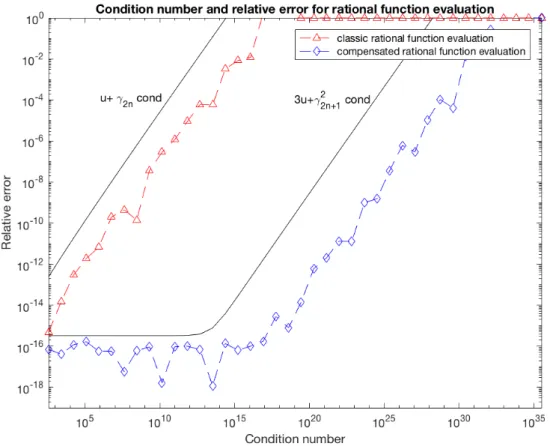
for x close to 1 and cond( fn, x) grows exponentially with respect to n. In the experiments reported on Figure1,
cond( fn, x) varies from 102 to 1035(for x = fl(1.333), that corresponds to the degree range n = 3, . . . , 42).
These huge condition numbers have some meaning since here the coefficients of pnand qn and the value x
are chosen to be exact floating-point numbers.
We experiment both RatEval and CompRatEval. For each rational function fn, the exact value fn(x) is
approximate with a high accuracy thanks to the Symbolic Math Toolbox of MATLAB. Figure1presents the relative accuracy ∣y − fn(x)∣/∣ fn(x)∣ of the evaluation y computed by the two algorithms.
Figure 1: Comparison of the accuracy of RatEval and CompRatEval
We observe that the compensated algorithm exhibits the expected behavior. The full precision solution is computed as long as the condition number is smaller than u−1≈ 1016. Then, for condition numbers between
u−1and u−2≈ 1032, the relative error degrades to no accuracy at all.
We now demonstrate the practical efficiency in terms of running time comparing our algorithm and up-to-date challenger.
Since Bailey’s double-double are usually considered as the most efficient portable library to double the IEEE-754 double precision, we consider it as a reference in the comparisons. Double-double numbers are represented as an unevaluated sum of a leading double and a trailing double. More precisely, a double-double number a is the pair (ah, al) of floating-point numbers with a = ah+ al and ∣al∣ ≤ u∣ah∣.
In the sequel, we present two algorithms to compute product of two double-double or a double times a double-double. Those algorithms are taken from [1].
Algorithm 6.1. Product of the double-double number (ah, al) by the double number b
function [ch, cl] = prod dd d(ah, al, b)
[sh, sl] = TwoProduct(ah, b)
[th, tl] = FastTwoSum(sh, (al ⊗ b))
[ch, cl] = FastTwoSum(th, (tl⊕ sl))
Algorithm 6.2. Addition of the double number b to the double-double number (ah, al)
function [ch, cl] = add dd d(ah, al, b)
[th, tl] = TwoSum(ah, b)
The double-double library can be used to implement an Horner scheme in quadruple precision like DDHorner.
Algorithm 6.3. Horner scheme with internal double-double computations
function res = DDHorner(p, x) sh= an sl = 0 for i = n − 1 ∶ −1 ∶ 0 [ph, pl] = prod dd d(sh, sl, x) [sh, sl] = add dd d(ph, pl, ai) end res= sh
With DDHorner, we can evaluate a rational function in quadruple precision.
Algorithm 6.4. Rational function evaluation with double-double Horner scheme
function res = DDRatEval(p, q, x)
res= DDHorner(p, x) ⊘ DDHorner(q, x)
We have implemented the three algorithms RatEval, CompRatEval, and DDRatEval in a C code to measure their overhead compared to the RatEval algorithm. We have programmed these tests straightforwardly with no other optimization than the ones performed by the compiler.
For each algorithm, we measured the ratio of its computing time over the computing time of the classic rational function evaluation algorithm. It turned out that our compensated algorithm CompRatEval is about 3 times slower than the classic Horner scheme. The same slowdown factor is about 10 for algorithm DDRatEval. From a practical point of view, we can state that our algorithm is about 5 times faster than the algorithm with double-doubles.
We compared RatEval, CompRatEval and DDRatEval in term of measured computing time. We tested with random rational functions where the degree of numerator and denominator vary from 100 to 100000.
Table 1: Measured computing times with RatEval normalised to 1.0
n RatEval CompRatEval DDRatEval
100 1.0 2.0 10.0 500 1.0 1.6 7.9 1000 1.0 1.7 8.2 10000 1.0 1.6 8.2 100000 1.0 1.6 8.5
7 Conclusion
We presented a fast algorithm for the evaluation of rational functions in floating-point arithmetic. We have proved that the accuracy of the result computed by our compensated algorithm is similar to the one given by the classic algorithm performed in doubled working precision. The only assumption we made is that the floating-point arithmetic available on the computer is conformed to the IEEE-754 Standard. Its low requirement make it highly portable, and our compensated algorithm could be easily integrated into numerical
libraries. Our algorithm uses only basic floating-point operations, and only the same working precision as the data. Finally, our compensated algorithm runs much more faster than existing implementation producing the same output accuracy. This approach can easily be generalized to rational functions where numerators and denominators are written in other basis and for bivariate rational functions (see [5,4,10,11] for example).
Acknowledgement
This work was partly supported by the project FastRelax ANR-14-CE25-0018-01.
References
[1] D. H. Bailey. A Fortran-90 double-double library, 2001. Available at URL =http://crd-legacy.lbl.
gov/~dhbailey/mpdist/.
[2] S. Boldo and J.-M. Muller. Some functions computable with a fused-mac. In Paolo Montuschi and Eric Schwarz, editors, Proceedings of the 17th Symposium on Computer Arithmetic, pages 52–58, Cape Cod, USA, 2005.
[3] T. J. Dekker. A floating-point technique for extending the available precision. Numer. Math., 18:224–242, 1971.
[4] P. Du, H. Jiang, and L. Cheng. Accurate evaluation of polynomials in legendre basis. J. Applied Mathematics, 2014:742538:1–742538:13, 2014.
[5] P. Du, H. Jiang, H. Li, L. Cheng, and C. Yang. Accurate evaluation of bivariate polynomials. In 17th International Conference on Parallel and Distributed Computing, Applications and Technologies, PDCAT 2016, Guangzhou, China, December 16-18, 2016, pages 51–56, 2016.
[6] S. Graillat, Ph. Langlois, and N. Louvet. Algorithms for accurate, validated and fast polynomial evaluation. Japan J. Indust. Appl. Math., 2-3(26):191–214, 2009. Special issue on State of the Art in Self-Validating
Numerical Computations.
[7] S. Graillat, N. Louvet, and Ph. Langlois. Compensated Horner scheme. Research Report 04, ´Equipe de recherche DALI, Laboratoire LP2A, Universit´e de Perpignan Via Domitia, France, 52 avenue Paul Alduy, 66860 Perpignan cedex, France, July 2005.
[8] N. J. Higham. Accuracy and stability of numerical algorithms. Society for Industrial and Applied Mathematics (SIAM), Philadelphia, PA, second edition, 2002.
[9] IEEE Computer Society. IEEE Standard for Floating-Point Arithmetic. IEEE Standard 754-2008, August 2008. Available athttp://ieeexplore.ieee.org/servlet/opac?punumber=4610933.
[10] H. Jiang, R. Barrio, H. Li, X. Liao, L. Cheng, and F. Su. Accurate evaluation of a polynomial in chebyshev form. Applied Mathematics and Computation, 217(23):9702–9716, 2011.
[11] H. Jiang, S. Li, L. Cheng, and F. Su. Accurate evaluation of a polynomial and its derivative in bernstein form. Computers & Mathematics with Applications, 60(3):744–755, 2010.
[12] D. E. Knuth. The Art of Computer Programming, Volume 2, Seminumerical Algorithms. Addison-Wesley, Reading, MA, USA, third edition, 1998.
[13] Y. Nievergelt. Scalar fused multiply-add instructions produce floating-point matrix arithmetic provably accurate to the penultimate digit. ACM Trans. Math. Software, 29(1):27–48, 2003.
[14] T. Ogita, S. M. Rump, and S. Oishi. Accurate sum and dot product. SIAM J. Sci. Comput., 26(6):1955–1988, 2005.