HAL Id: hal-02001008
https://hal.archives-ouvertes.fr/hal-02001008
Submitted on 6 Feb 2019
HAL is a multi-disciplinary open access
archive for the deposit and dissemination of sci-entific research documents, whether they are pub-lished or not. The documents may come from teaching and research institutions in France or abroad, or from public or private research centers.
L’archive ouverte pluridisciplinaire HAL, est destinée au dépôt et à la diffusion de documents scientifiques de niveau recherche, publiés ou non, émanant des établissements d’enseignement et de recherche français ou étrangers, des laboratoires publics ou privés.
locomotion
Olivier Stasse, Kevin Giraud-Esclasse, Edouard Brousse, Maximilien Naveau,
Rémi Régnier, Guillaume Avrin, Philippe Souères
To cite this version:
Olivier Stasse, Kevin Giraud-Esclasse, Edouard Brousse, Maximilien Naveau, Rémi Régnier, et al.. Benchmarking the HRP-2 humanoid robot during locomotion. Frontiers in Robotics and AI, Frontiers Media S.A., 2018, 5, �10.3389/frobt.2018.00122�. �hal-02001008�
Benchmarking the HRP-2 humanoid robot
during locomotion
Olivier Stasse1,∗, Kevin Giraud-Esclasse1, Edouard Brousse2, Maximilien Naveau3, R ´emi R ´egnier2, Guillaume Avrin2, and Philippe Sou `eres1
1Laboratoire d’Analyse et d’Architecture des Syst `emes, (LAAS) CNRS, Universit ´e
de Toulouse, France
2Laboratoire Nationale de M ´etrologie et d’essais (LNE), Paris, France
3Max-Planck Institute (MPI), Tuebingen, Germany
Correspondence*: Corresponding Author [email protected]
ABSTRACT 2
In this paper we report results from a campaign of measurement in a laboratory allowing to
3
put a humanoid robot HRP-2 in a controlled environment. We have investigated the effect of
4
temperature variations on the robot capabilities to walk. In order to benchmark various motions
5
modalities and algorithms we computed a set of performance indicators for bipedal locomotion.
6
The scope of the algorithms for motion generation evaluated here is rather large as it spans
7
analytical solutions to numerical optimization approaches able to realize real-time walking or
8
multi-contacts.
9
Keywords: benchmarking, bipedal locomotion, humanoid robot HRP-2, controlled environment, numerical optimization, walking
10
1
INTRODUCTION
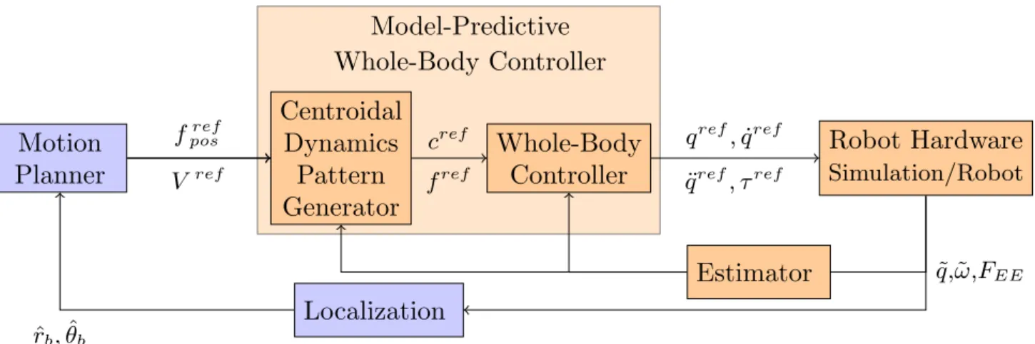
Model-Predictive Whole-Body Controller Motion Planner Centroidal Dynamics Pattern Generator Whole-Body Controller Estimator Localization Robot Hardware Simulation/Robot fposref V ref cref fref qref, ˙qref ¨ qref, τref ˜ q,˜ω,FEE ˆ rb, ˆθbFigure 1. General architecture to generate motion for a humanoid robot. In this paper the boxes in orange are the one benchmarked, whereas the blue boxes are not benchmarked
From the seminal work of Chestnutt (2010) to the recent methods proposed in the frame of the Darpa
11
Robotics Challenge (DRC) Tsagarakis et al. (2017); Lim et al. (2017); Radford et al. (2015); Johnson
12
et al. (2017); Marion et al. (2017); DeDonato et al. (2017), humanoid robots are moving using a control
13
architecture following the general framework depicted in Fig. 1. Based on an internal representation of
14
the environment and the localization of the robot (ˆrb and ˆθb being respectively the base position and
15
orientation), the Motion Planner (MP) plans a sequence of reference end-effector contact positions (fref),
16
or a reference center of mass linear velocity combined with a reference waist angular velocity (Vref).
17
These references are then provided to a Model-Predictive Whole-Body Controller (MPWBC) which
18
generates a motor command for each joint (joint torques (τref), positions (qref), velocities ( ˙qref) and
19
accelerations (¨qref)). This block is critical in terms of safety as it maintains the dynamics feasibility of
20
the control and the balance of the robot. The Model-Predictive Whole-Body Controller (WBC) can be
21
expressed as a unique optimal control problem but at the cost of efficiency in terms of computation time
22
or solution quality. This is why this controller is usually divided in two. First trajectories for the robot
23
center of mass cref and the positions of contacts with the environment fref are found using a Centroidal
24
Dynamics Pattern Generator (CDPG). And, in turn a WBC computes an instantaneous controller that
25
tracks these trajectories. More details about the CDPG can be found in the next paragraph. The whole
26
body reference is in turn sent to the Robot Hardware, which can be either the simulation or the real robot.
27
The feedback terms are based upon the measurements of the different sensors. The encoders evaluate
28
the joint position (˜q). The inertial measurement unit (IMU) measures the angular velocity (˜ωIM U) and
29
the linear acceleration (˜aIM U) of the robot torso, which give us information about the orientation of the
30
robot with respect to the gravity field. Finally the interaction with the environment is provided by the
31
force sensors classically located at the end-effectors (FEE ∈ {FRF, FLF, FRH, FLH} where the subscripts
32
have the following meaning EE: end-effector, RF : right foot, LF : left foot, RH: right hand, LH: left
33
hand). All these information are treated in an Estimator to extract the needed values for the different
34
algorithm. Finally the Localization block is dedicated to locate as precisely as possible the robot in its
35
3D environment, Various implementations of this architecture have been proposed with various levels of
36
success from the highly impressive Boston Dynamics System, to robots widely available such as Nao.
37
An open question is the robustness and the repeatability of such control system as well as its performance.
38
In this paper we propose a benchmarking of the HRP-2 robot in various set-ups and provide performance
39
indicators in scenarios which are possibly interesting for industrial scenarios.
40
The paper is structured as follows, first the paragraph 2 presents the related work on control and
41
benchmarking for humanoid robots, then paragraph 3 depicts our precedent contribution in the Koroibot
42
project and how it relates to this work, to continue, paragraph 4 lists the materials and different methods
43
used to perform the benchmarking, in turn the paragraph 5 shows the experimental results using the
44
indicators from paragraph 4, and finally the conclusion 6 summaries the contributions and results from this
45
paper.
46
2
RELATED WORK
In this paragraph we present the work that has been done relative to the control and the benchmarking of
47
humanoid robots.
48
2.0.1 Motion generation for humanoid robots
49
The different benchmarks included in this paper relate to MPWBC sketched in Fig. 1, so this section
50
is dedicated to its related work. Several techniques are used to mathematically formulate this problem.
t CoM
ˆ q
Balance, and Centroidal Momentum
WBC Locomotion problem degrees of freedom
Figure 2. Representation of the size of the locomotion problem. The abscissa represent the duration of the predicted horizon and the ordinate the number of robot DoF.
For instance hybrid-dynamics formulations as proposed by Grizzle et al. (2010) or Westervelt et al.
52
(2007) are efficient but difficult to generalize. The approaches used in this paper are based on mathematical
53
optimization which is broadly used in the humanoid robotics community. More precisely, the problem of the
54
locomotion can be described as an Optimal Control Problem (OCP). The robot generalized configuration
55
(qref) and velocity ( ˙qref) usually compose the state (x). The future contact points can be precomputed
56
by a Motion Planner or included in the state of the problem. The control of this system u, can be the
57
robot generalized acceleration (¨qref), the contact wrench (φk with k ∈ {0, . . . , Number of Contact}), or
58
the motor torques (τref). We denote by x and u the state and control trajectories. The following optimal
59
control problem (OCP) represents a generic form of the locomotion problem:
60 min x, u S X s=1 Z ts+∆ts ts `s(x, u) dt (1a) s.t. ∀t ˙x = dyn(x, u) (1b) ∀t φ ∈ K (1c) ∀t x ∈ Bx (1d) ∀t u ∈ Bu (1e) x(0) = x0 (1f) x(T ) ∈ X∗ (1g)
where ts+1 = ts+ ∆tsis the starting time of the phase s (with t0= 0 and tS = T ). Constraint (1b) makes
61
sure that the motion is dynamically consistent. Constraint (1c) enforces balance with respect to the contact
62
model. Constraints (1d) and (1e) impose bounds on the state and the control. Constraint (1f) imposes the
63
trajectory to start from a given state (estimated by the sensor of the real robot). Constraint (1g) imposes
64
the terminal state to be viable Wieber (2008). The cost (1a) is decoupled `s(x, u) = `x(x) + `u(u) and its
65
parameters may vary depending on the phase. `xis generally used to regularize and to smooth the state
66
trajectory while `utends to minimize the forces. The resulting control is stable as soon as `xcomprehends
67
the L2 norm of the first order derivative of the robot center of mass (CoM), Wieber et al. (2015).
68
Problem (1) is difficult to solve in its generic form. And specifically (1b) is a challenging constraint.
69
Most of the time the shape of the problem varies from one solver to another only by the formulation of
70
this constraint. The difficulty is due to two main factors: 1) There is a large number of degrees of freedom
(DoF). In practice we need to compute 36 DoF for the robot on a preview window with 320 iterations (1.6s)
72
to take into account the system inertia. 2) The system dynamics is non linear. Fig. 2 depicts the structure of
73
problem. To be able to solve the whole problem, represented by the full rectangle in Fig. 2 researchers used
74
nonlinear optimization. In this paper we evaluated a resolution of the MPWBC based on the formulation
75
given by Eq. 1. In this approach described in Koch et al. (2014), the authors computed a dynamical step over
76
motion with the HRP-2 robot, but this process can take several hours of computation. So simplifications
77
are necessary, for example Tassa et al. (2014), Koenemann et al. (2015) uses simplifications on the contact
78
model. This method is very efficient but is not suitable for complex contacts during walking for example.
79
Seminal works (Orin et al. (2013),Kajita et al. (2003b)) show that (1b) can be divided in two parts, the
80
non-convex centroidal dynamics (horizontal gray rectangle in Fig. 2) (Orin et al. (2013)) with few DoF
81
and the convex joint dynamics (vertical gray rectangle in Fig. 2). Kuindersma et al. (2014) and Sherikov
82
(2016) chose to deal the two gray part of Fig. 2 at once. They optimize for the centroidal momentum on
83
a preview horizon and the next whole body control. Qiu et al. (2011), Rotella et al. (2015), Perrin et al.
84
(2015) decouple the two separated gray rectangles in Fig. 2. They solve first for the centroidal momentum
85
and then for the whole body control. In general the centroidal momentum is still difficult to handle due
86
to its non-convexity. Finally Kajita et al. (2003a), Herdt et al. (2010), Sherikov et al. (2014) linearize
87
the centroidal momentum which provides a convex formulation of the locomotion problem. In Deits and
88
Tedrake (2014), the problem was formulated has a mixed-integer program (i.e. having both continuous and
89
discrete variables) in case of flat contact. In Mordatch et al. (2012), the same problem was handled using a
90
dedicated solver relying on a continuation heuristic, and used to animate the motion of virtual avatars.
91
2.1 Benchmarking 92
Different methods exist to benchmark robot control architectures, in del Pobil et al. (2006) the authors
93
argue that robotic challenges are an efficient way to do so. For example, the results of the DARPA
94
Robotics Challenge published in the Journal of Field Robotics special issues Iagnemma and Overholt
95
(2015) and Spenko et al. (2017), show the different control architecture in a determined context. Each
96
behavior successfully accomplished grants point to the team and the best team won the challenge. This
97
benchmarking was however costly as the robots had no system to support them in case of fall. In addition,
98
as it is mostly application driven it is necessary in evaluating the system integration but not the independent
99
subparts.
100
For the specific case of motion generation, it has been recently proposed by Brandao et al. (2017) to
101
use a scenario called ”Disaster Scenario Dataset”. It allows benchmarking posture generation (solved by
102
the WBC) and trajectory generation (MPWBC) using optimization. A set of problems is proposed by
103
means of foot steps locations(FRF, FLF). From this it is possible to compare algorithms realizing the
104
two functionnalities (WBC and MPWBC). The evaluation is realized in simulation using the Atlas robot
105
and the ODE dynamic simulator. This first step is necessary but one step further is to benchmark a real
106
humanoid platform. For this paper we used a more systematic decomposition of the humanoid bipedal
107
locomotion Torricelli et al. (2015). Further description can be found in paragraph 4.7. This paper focuses
108
on evaluating the MPWBC and WBC on the Robot Hardware. The Estimator used in this context is
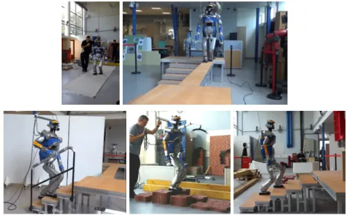
109
important but it is reflected in the stabilization process. The Motion Planning is not evaluated here as the
110
planned motion is always the same or solved at the MPWBC level. The Localization is provided by a
111
motion capture system.
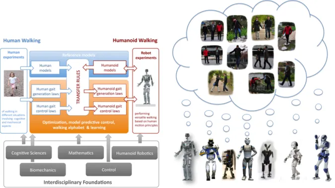
Figure 3. (left) Graphical representation of the scientific approach of the Koroibot project - (right) View of the humanoid robot used in the Koroibot project dreaming of human walking capabilities
3
THE KOROIBOT PROJECT AND OUR PRIOR CONTRIBUTIONS
The work presented in this paper takes its root in the context of the European project Koroibot (http:
113
//www.koroibot.eu/).
114
3.0.1 General purpose
115
The goal of the Koroibot project was to enhance the ability of humanoid robots to walk in a dynamic and
116
versatile way, and to bring them closer to human capabilities. As depicted in Fig. 3-(left), the Koroibot
117
project partners had to study human motions and use this knowledge to control humanoid robots via
118
optimal control methods. Human motions were recorded with motion capture systems and stored in an open
119
source data base which can be found at https://koroibot-motion-database.humanoids.
120
kit.edu/. With these data several possibilities were exploited:
121
Criteria that humans are assumed to minimize using Inverse optimal control.
122
Transfer from human behaviors to robots was done with walking alphabets and learning methods
123
Mandery et al. (2016).
124
These human behavior was safely integrated in robots applying optimal controllers.
125
Design principles were derived for new humanoid robots. Mukovskiy et al. (2017); Clever et al. (2017)
126
3.0.2 The robot challenges
127
In order to evaluate the progress of the algorithms at the beginning and at the end of the project, a set
128
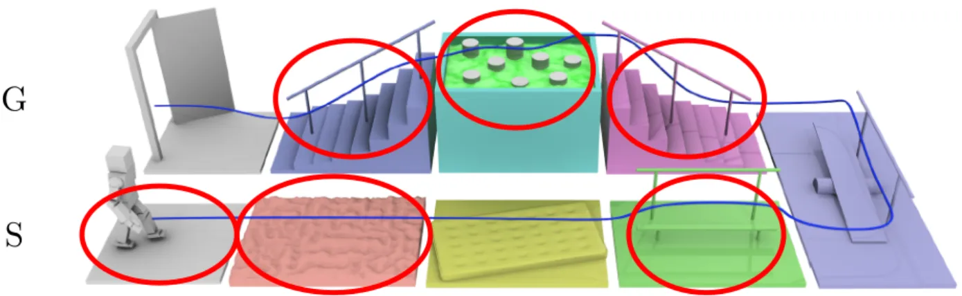
of challenges were designed focusing specifically on walking (see Fig. 4). Fig. 3-(right) shows all the
129
robot hosted by the various partners. All the team owning a robot had to perform some of these challenges
130
considering the current and potential state of their robots and controllers.
S
G
Figure 4. Challenges of the Koroibot project. In red the challenges chosen by the LAAS-CNRS.
3.0.3 The Key Performance Indicators (KPI)
132
In this context and in collaboration with the H2R project, a detailed set of key performance indicators
133
(KPI) have been proposed Torricelli et al. (2015). These KPI try to capture all the bipedal locomotion
134
patterns. Specific sub-functions of the global motor behaviors were analyzed (see Fig. 5-(right)). The results
135
are expressed as two different sub-function sets. First, the sub-functions associated to body posture task
136
with no locomotion. And second the same sub-functions but including the robot body transport. The initial
137
condition may vary depending on the experiment to perform. This is the idea of the intertrial variability. The
138
sub-functions are also classified by taking into account the changes in the environment or not. Each of these
139
functions can be evaluated for different robots using the criteria depicted in Fig. 5-(left). The performance
140
are classified in two sub categories, quantitative performance and human likeness. In addition there are
141
indications on the last two columns if the criteria is applicable on a standing task or on a locomotion task.
142
Again, all the team owning a robot had had to perform an evaluation of these KPI, considering the current
143
and potential state of their robots and controllers.
144
3.1 The work done in the Koroibot context 145
In the Koroibot context the gepetto team evaluated the KPI one the robot HRP-2 (second robot from the
146
left in (Fig. 3-(right)). Among the challenges presented in Fig. 4, we considered the following ones:
147
walking on a flat ground,
148
walking on an uneven ground,
149
walking on a mattress,
150
walking on a beam without handrail,
151
climbing a stair case with/without handrail,
152
walking on stepping stones,
153
going down a stair case without handrail,
154
They are depicted by red circles in Fig. 4. In addition to these challenges we added the perturbation
155
rejection. Considering the selected challenges we picked the following KPI sub-function:
Abilities Benchmarks
Name Description Benchmark Applicability
Posture Transport P er fo rm an ce S ta bi lit y Intratrial
Stability Ability to Maintain EquilibriumWithin a Single Trial
Time Until Falling X
Cycles Until Falling X X
Intertrial
Stability Ability to Maintain the EquilibriumAcross Different Trials Success Rate Across NDifferent Trials X X
Gross Body
Equilibrium Ability to Maintain Equilibrium Overthe Base of Support
Energy Stability Margin
(ESM) X Maximum Accepted Disturbance Amplitude X X Maximum Accepted Disturbance Frequency X X E ffi ci en cy Global Energy
Consumption Ability to Transport Body with LowEnergetic Costs
Specific Energetic cost
of Transport Cet X
Specific Mechanical Cost
of Transport Cmt X
Passivity Ability to Minimize J oint TorquesDuring Walking Passive Gait Measure(PGM) X
Reaction Time Disturbance or External CommandAbility to Promptly React to Time from Input and
Initiation of Motor Action X X
H um an Li ke ne ss K in em at ic s Gross Body
Motion Motion of the Whole Body Expressedby Global Variables
CoM Trajectory (Correlation, Dynamic Time
Warping) X X
Gait Harmony X
Body Sway (Frequency
Response Function) X
Natural Looking Motion X X
Individual J oint
Motion Motion of the Single J oints or LimbsTaken Separately
J oint Trajectory (Correlation, Dynamic Time
Warping) X X
Knee, Ankle Forefoot Rocker X
Interlimb
Coordination Ability to Coordinate BetweenDifferent Body Parts
Symmetry (Ratio Index) X X
Trunk/Arm Motion X X
Intralimb
Coordination Ability to Move Multiple J oints of theSame Limb Coordinately Kinematic Synergies X X
D yn am ic s Gross Body
Kinetics Forces Exerted Between the WholeBody and the Environment
Ground Reaction Forces (Correlation, Dynamic Time
Warping) X X
Single-J oint
Kinetics Force Exerted Among Limbs J oint Torques (Correlation,Dynamic Time Warping) X X
Dynamic Similarity
Ability of Having Leg Pattern Dynamically Similar to Most Legged
Animals
Froude Number (Dimensionless Gait
Velocity) X
Dynamicity Ability to Use Falling State for BodyProgression Dynamic Gait Measure(DGM) X
External
Compliance Ability to Respond Resiliently toExternal Disturbances Impulse ResponseFunction (IRF) X X
Internal
Compliance Ability to Store and Release Energy Active/Net J oint Torque X X
Function
Body Posture Body Transport
E nv iro nm en t S ta tio na ry In te rt ria l V ar ia bi lit y N o
Static Horizontal Surface Horizontal Ground atConstant Speed
Static Inclined Surface
Sloped Ground
Stairs
Y
es Different Static Surfaces
Variable Slopes Irregular Terrain Slippery Surface In M ot io n
Continuous Surface Tilts Treadmill at Constant Speed
Continuous Surface
Translations Soft Terrain with ConstantCompliance
Bearing Constant Weight Bearing Constant Weight
Pushes Pushes
Sudden or Pseudorandom
Surface Tilts Treadmill at Variable Speed(Including Start-Stop)
Sudden Surface Translations Seesaw
Body Sway Referenced
Platform (BSRP) Soft Ground with VariableCompliance
In te rt ria l V ar ia bi lit y N o Y es
Figure 5. (left) Performances indicators (right) The motor skills considered in the benchmarking scheme. This scheme is limited to bipedal locomotion skills. The concept of intertrial variability represent modifications of the environment between trials. (dashed) Motor skills evaluated in Naveau (2016) (not dashed) Motor skills evaluates in this paper.
horizontal ground at constant speed,
157
stairs,
158
bearing constant weight (the robot’s own weight)
159
success rate across N different trials,
160
mechanical energy,
161
mechanical plus electrical energy,
162
All these choices are shown in Fig. 5 by red ellipses on the table. The mathematical details and results
163
are presented below in paragraph 4.7.
164
4
MATERIALS AND METHODS
In this paragraph the experimental setups used to compute each of the performance indicators given in 4.7
165
are described. It also presents the motor skills given in Fig. 5 and their implementation. In addition to this,
166
the algorithms used to perform the different test are depicted in paragraph 4.8.
167
4.1 Different temperatures 168
LNE is equipped with temperature varying rooms which allowed us to quantify some of the performance
169
indicators between 5◦C and 45◦C. In this way, we evaluated the robustness and limits of our robot for all
(b) (a)
(c)
Figure 6. Pictures of the experimental setup at LNE (a) the robot hang up to walk on a slope (b) the
translational plate (c) the temperature controlled chamber (end of the robot climbing 15 cm at 10◦C)
the performance indicators. It appeared that the robot behavior deteriorates at low temperatures. At 5◦C it
171
was not possible to perform the calibration procedure as the robot could not move. At 10◦C the friction
172
are sufficiently low such that the robot could move. Another phenomena occurs above 40◦C: thermal
173
protection prevents the robot from moving if the temperature is too high. This happens at 40◦C after few
174
motions due to internal temperature build up. In this room, apart from these extreme cases, the motions and
175
indicators measurements have be performed as expected on a flat ground or on the stairs from the Koroibot
176
project. This staircase is made of 4 stairs and a platform with each stair separated by 15 cm height. The
177
dimension of one stair case is 1 m × 0.25 m × 0.05 cm.
178
4.2 Tilted surfaces 179
In the context of the body skills in motion, we considered tilting surfaces. This was tested with the
180
stabilizer commercially available with HRP-2. The setup is a platform which can be tilted upward and
181
downward on one side with an hydraulic actuator. The surface was tilted continuously until the robot fell
182
off. On the other hand, we tested walking algorithms with different angles (pointing up or down) until the
183
robot fell down. Tests were realized with the robot pointing down, pointing up and across the slope. In
184
Fig. 5 this corresponds to Body Posture - Continuous Surface Tilts.
185
4.3 Horizontal translations 186
We used a mobile plate controlled in the horizontal plane to perform continuous oscillating surface
187
translations at various frequencies and various amplitudes. The platform was using a hydraulic actuator.
188
The aim was to find the frequency and the amplitude that the controlled robot is able to sustain. In Fig. 5
189
this corresponds to Body Posture - Continuous Surface translations.
190
4.4 Bearing 191
In order to test bearing weights with the robot, we added bags of 5 kgs to 15 kgs in such way that the
192
robot balance is maintained. This approach is a bit limited as they are several ways to bear a weight. Indeed
193
it can be done with a backpack, in collaboration with someone, by holding the object against its chest. Each
of this approach comes with its own specific constraint. In order to avoid such constraints, we decided to
195
take the most simplest choice and hang soft weights on the front and the back of the chest. In Fig. 5 this
196
corresponds to Body Transport - Bearing Constant Weight.
197
4.5 Pushes 198
This paragraph presents the pushes experiments. We tried to find the sufficient force to make the robot
199
fall down. This was achieved by using a stick on top of which was fixed a force sensor displaying the
200
maximum force measured during a physical interaction. The experience was realized while the robot was
201
standing and walking. The force was applied in the sagittal and frontal planes until making HRP-2 fall. The
202
force was applied behind the waist of the robot. This part of HRP-2 was made specifically soft to support
203
impacts. The walking part is the most difficult in terms of repeatability as the robot might be in different
204
foot support and therefore be less stable depending on the situation. In Fig. 5 this corresponds to Body
205
Posture - Pushes and Body Transport - Pushes.
206
4.6 Data 207
A CAD model of this staircase used is available on the github repository where all the log
208
of the experiments are also present: https://github.com/laas/koroibot KPI. All the computation
209
performed on the logs and implementing the key performance indicators are available here:
210
https://github.com/laas/EnergyComputation.
211
4.7 Key Performance indicators (KPI) 212
In this section the performance indicators used to evaluate the humanoid robot HRP-2 are described.
213
They are mostly based on the work proposed in Torricelli et al. (2015). In the Koroibot project we used key
Figure 7. Sample of the experimental setup of the Koroibot project in LAAS-CNRS
214
performance indicators (KPI) to analyze the behavior of the robot at the beginning and at the end of the
215
project. These results lead us toward the improvements to be made. In 2013 the algorithm mostly used and
216
implemented on HRP-2 in LAAS-CNRS where the walking pattern generators described in Morisawa et al.
217
(2007) and in Herdt et al. (2010). The performance indicators chosen were:
The execution time TM = tend− tbegin, where tbeginis found when the sum of the norm of the motor 219
axis velocities reaches 6 rad s−1for the first time in the log and tendis when the sum of the norm of
220
the motor axis velocities is below 0.5 rad s−1.
221
The walked distance, being the distance between the final base position and the first one. The base
222
pose is reconstructed using an odometry with the joint positions only. The drift of this odometry is
223
8cm over a 3.6m during a straight walk.
224
The success rate, being the number of time a specific task could be performed without fall, over the
225
total number of trial of the task.
226
The maximum tracking error from the planned trajectory, T rackingError(t) =
Z t+0.1
t
|qref − ˜q|dt/0.1
M axT rackingError = max
t (T rackingError(t))
with T rackingError being the average normed difference between the desired joint trajectory
227
(qref) and the joint pose measured from the encoder (˜q) during 0.1s starting at time t. And
228
M axT rackingError being the maximum value of the T rackingError function.
229
The mechanical energy consumed normalized over the walking distance D and the execution time
TM.
Emechanical =
Z tend
tbegin
|τ ω|dt/(TM D)
with Emechanical being the integral over time of the mechanical power, τ being the torques applied at
230
the robot joints and ω being the velocity of the robot joints
231
The electrical energy dissipated by the motor resistance normalized over the walking distance D and
the execution time TM,
Emotor resistance = Z tend tbegin R i2dt/(TM D) = Z tend tbegin R kc2τ2dt/(TM D)
with Emotor resistancebeing the integral over time of the electric power dissipated, R being the motor
232
resistances, kc being the electric motor torque constant and τ being again the torques applied at the
233
robot joints.
234
The total energy consumed during the walking distance D and the execution time TM,
Etotal = Emechanical + Emotor resistance+ Eelectronics
with Etotalbeing the sum of the energy consumed by the system normalized over the walking distance
D and the execution time TM, and Eelectronicsbeing the energy consumed by the on-board electronic
cards. Eelectronicsis neglected in this study so:
The mechanical cost of transport and the total cost of transport, Emechanical cost transport =
Z tend
tbegin
|τ ω|dt/(m g D)
Etotal cost transport =
Z tend tbegin |τ ω|dt + Z tend tbegin R kc2τ2dt ! /(m g D)
with Emechanical cost transport and Etotal cost transport being the respectively the mechanical and total
235
cost of transport, m being the total mass of the robot, and g = 9.81ms−2the gravity constant.
236
The Froude number,
Fr = v √ gl v = D TM
where v is the robot center of mass mean velocity along the horizontal plane,, and l is the leg length.
237
This number represents the ratio between the kinetic energy and the potential energy. It can also be
238
interpreted as an indicator on the stepping frequency.
239
The trajectories were generated off line and repeatedly played on the robot to analyze their robustness.
240
Views of the experimental setups can be seen in Fig. 7.
241
4.8 Motion generation for humanoid robots locomotion 242
This section explains the links between the motion generation architecture depicted in Fig.1 and the
243
Key Performance Indicators given in the paragraph 4.7. The set of function entitled body posture depicted
244
in Fig.1-(right) represents the behavior which is provided by what is called a whole-body controller. It
245
consists in two parts:
246
• an estimator, which provides the orientation of the robot with respect to the gravity field and the
247
positions of the end-effectors in contact with the environment.
248
• a whole-body controller which guarantee that the robot balance is maintained with respect to cref,
249
fref and possibly a qref.
250
In this paper we have evaluated independently only one whole body motion controller. It is the stabilizer
251
provided by Kawada Inc. We give detailed performances evaluation of this controller in the experimental
252
part of this paper. It was described in various paper such as Kajita et al. (2007) and Kajita et al. (2001).
253
The set of function entitled body transport depicted in Fig.1-(right) in this paper are four CDPG and
254
one MPWBC. The four CDPG evaluated in this paper are the following ones: Carpentier et al. (2016),
255
a multi-contact centroidal dynamic pattern generator used to climb stairs with given contact positions,
256
Kajita et al. (2003a) the original walking pattern generator implemented by Shuuji Kajita with given
257
foot steps, Morisawa et al. (2007) an analytical walking pattern generator allowing immediate foot step
258
modifications, Naveau et al. (2017) a real time non linear pattern generator able to decide autonomously
259
foot-steps positions. In each case the goal of the CDPG is to generate a center of mass trajectory and
260
the foot-steps trajectories. For Kajita et al. (2003a), Naveau et al. (2017), and Morisawa et al. (2007) a
261
dynamical filter is used to correct the center of mass trajectory to improve the dynamical consistency of
the motion. In each case, a whole body motion generator (not to be confused with a whole body motion
263
controller) is used without feedback to generate the reference position qref, and the desired zref which is
264
then send to the stabilizer. For Naveau et al. (2017) and Morisawa et al. (2007) we used the stack of task
265
described in Mansard et al. (2009) as a Generalized Inverse Kinematics scheme. In Carpentier et al. (2016)
266
a Generalized Inverse Dynamics was used to generate the reference value for qref and cref. The MPWBC
267
provides directly the controls. The one used is from Koch et al. (2014) using the Muscod-II Diehl et al.
268
(2001) nonlinear solver.
269
5
EXPERIMENTS
In this paragraph we present the numerical results obtained from the computation of the KPI explained in
270
details in paragraph 4.7 for each set of experiments. As a reminder here the list of the KPI:
271
walked distance,
272
success rate,
273
max tracking error,
274
duration of the experiment,
275
mechanical joint energy,
276
actuators energy,
277
cost of transport,
278
mechanical cost of transport,
279
Froude number.
280
A video displaying a mosaic of all the experiments is available at the following URL:
281 https://www.youtube.com/watch?v=djWGsb44JmY&feature=youtu.be. 282 5.1 Climbing stairs 283 5.1.1 Stairs of 10 cm 284
In this experiment, the humanoid robot HRP-2 is climbing stairs of 10 cm height without any handrail.
285
The difficulty of this task is that the robot has to do quite large steps and to perform vertical motion.
286
Because of the large motion issue the robot is climbing one stair at a time. Which means that the robot put
287
one foot on the next stair and the other on the same stair. This avoid a too large joint velocity that the robot
288
could not track.
289
Morisawa et al. (2007) CDPG was evaluated at the beginning of the project although the variation of
290
height violates the assumption of the cart table model. But thanks to the dynamical filter the motion
291
generated was sufficiently dynamically consistent so that the stabilizer could cope with the situation. The
292
test was performed in a room at 20◦C. The KPI results can be seen in Fig. 11-(tool upstairs).
293
The other test was performed at the end of the project on the CDPG Carpentier et al. (2016). This time
294
the CDPG took into account the center of mass height variation but not the whole body motion. The
295
stabilizer should theoretically less trouble to compensate for the simplifications made. For Carpentier et al.
296
(2016) three different temperatures were tested: 10◦C, 20◦C and 35◦C. The numerical results are depicted
297
in Fig. 8.
298
Interestingly, the temperature level has a direct impact in terms of mechanical cost as it diminishes with
299
the increase in temperature. It is reflected in the tracking error. This intertrial variation do not come from
10°C 20°C 35°C m 1.73 nb:4 1.71 nb:4 1.73 nb:5 Walked distance 10°C 20°C 35°C 100 8 × 101 9 × 101 Dimensionless 0.80 nb:4 0.80 nb:4 1.00 nb:5 Success rate 10°C 20°C 35°C 6 × 10³ 7 × 10³ 8 × 10³ rad 7.23E-03 nb:4 6.52E-03 nb:4 6.13E-03 nb:5
Max tracking error
10°C 20°C 35°C 101
102
s 20.00
nb:4 20.00 nb:4 20.00 nb:5
Duration of the experiment
10°C 20°C 35°C 6 × 101 7 × 101 8 × 101 J.m-1.s-1 73.91 nb:4 68.65 nb:4 60.62 nb:5 Mechanical energy 10°C 20°C 35°C 2 × 10² J.m-1.s-1 180.21 nb:4 169.70 nb:4 160.29 nb:5 Total energy 10°C 20°C 35°C 6 × 100 7 × 100 Dimensionless 6.43 nb:4 6.06 nb:4 5.72 nb:5
Total cost of transport
10°C 20°C 35°C Dimensionless 2.64 nb:4 2.45 nb:4 2.16 nb:5
Mechanical cost of transport
10°C 20°C 35°C Dimensionless 3.55E-02 nb:4 3.50E-02 nb:4 3.56E-02 nb:5 Froude number Algorithm : 10cm
Figure 8. Climbing 10 cm stairs without handrail
the change of reference trajectory as it is strictly the same for every trial. There is a level of adaptation due
301
to the stabilizer, but each temperature has been tested at least 4 times. A possible explanation is the fact
302
that the grease in the harmonic drive generate less friction with higher temperature.
303
As the cost of transport is dimensionless it allows to compare the two motions regardless of their duration.
304
It is then interesting to see that the cost of transport in Fig. 11-(tool upstairs) and in Fig. 8-(10◦C) are
305
very similar. And that at the same temperature the total cost of transport for Carpentier et al. (2016)
306
CDPG is 9.6% better (from 6.71 to 6.06). One explanation is that the motion from Carpentier et al. (2016)
307
CDPG being more dynamically consistent, the stabilizer consume less energy to compensate for the model
308
simplifications.
309
5.1.2 Stairs of 15 cm
310
In this experiment, the humanoid robot HRP-2 is climbing stairs of 15 cm height using a handrail. In
311
addition the robot is not using any stabilization algorithm, because there are non-coplanar contacts.
312
In this setup the Morisawa et al. (2007) CDPG has to be used without handrail because of the model
313
simplifications. Trials has therefore been done using a WBC (described in Mansard et al. (2009)) without
314
the handrail. The results show that the current demanded by the motors went up to 45 A. And because the
315
HRP-2 batteries can not provide more than 32 A, all trial failed. This is the reason why the results are not
316
shown in this study.
317
Nevertheless, tests using the handrail could be performed with Carpentier et al. (2016) CDPG. The
318
corresponding results are depicted in Fig. 9. It confirms that the energy is decreasing with the increase of
319
temperature without the stabilizer. Note that the energy spend by the robot is clearly higher than for the
320
experience on the 10 cm stairs, i.e. a 36% of increase for the energy of walking.
10°C 20°C 35°C 40°C 8 × 101 m 0.75 nb:4 0.75 nb:3 0.75 nb:5 0.75 nb:5 Walked distance 10°C 20°C 35°C 40°C 100 4 × 101 6 × 101 Dimensionless 0.40 nb:4 0.50 nb:3 1.00 nb:5 1.00 nb:5 Success rate 10°C 20°C 35°C 40°C 102 9 × 10³ rad 9.59E-03 nb:4 9.62E-03 nb:3 9.11E-03 nb:5 9.51E-03 nb:5
Max tracking error
10°C 20°C 35°C 40°C 101
102
s 20.00
nb:4 20.00 nb:3 20.00 nb:5 20.00 nb:5
Duration of the experiment
10°C 20°C 35°C 40°C 102 9 × 101 J.m-1.s-1 100.50 nb:4 97.39 nb:3 92.99 nb:5 90.75 nb:5 Mechanical energy 10°C 20°C 35°C 40°C 3 × 10² J.m-1.s-1 301.04 nb:4 289.00 nb:3 284.09 nb:5 284.40 nb:5 Total energy 10°C 20°C 35°C 40°C 101 Dimensionless 10.75 nb:4 10.32 nb:3 10.14 nb:5 10.15 nb:5
Total cost of transport
10°C 20°C 35°C 40°C Dimensionless 3.59 nb:4 3.48 nb:3 3.32 nb:5 3.24 nb:5
Mechanical cost of transport
10°C 20°C 35°C 40°C
Dimensionless
1.54E-02
nb:4 1.54E-02 nb:3 1.53E-02 nb:5 1.53E-02 nb:5
Froude number Algorithm : 15cm
Figure 9. Climbing 15 cm stairs with a handrail
5.1.3 Stepping Stones
322
In this experience, the humanoid robot HRP-2 had to go up and down on stairs made of red interlocking
323
paving stones. Between each stairs there is a height difference of ±5 cm. It is using the CDPG described
324
in Morisawa et al. (2007). It is slightly different from the previous experiments because there are holes
325
between the stairs. To cope with this, the generated trajectories had to always change the height of the next
326
support foot. As the paving stones were always slightly moving due to the robot weight the balance was
327
difficult to obtain in a reliable way. As indicated in the graph depicted in Fig.11, despite a success rate
328
of 1, the tracking error reaches a level (8e−03). This tracking error is greater than the one obtained by the
329
10 cm climbing experiment at 10◦C but lower than the one obtained by the 15 cm climbing experiment
330
at 35◦C (which is the lower for this temperature and the CDPG). A possible explanation why the energy
331
consumption is greater is greater than the 10 cm climbing stairs is mostly due to the unstability of the
332
stones and the fact that in this experiment the robot climb the stairs in a human fashion, i.e not one stair at
333
a time.
334
5.2 Walking on a beam 335
This experiments was realized using the CDPG Morisawa et al. (2007). In this experiment the humanoid
336
robot HRP-2 is walking on a beam. Initially, the experiment success rate on a real beam was around 20 %.
337
This rate was improved to achieve a 90 % success rate, thanks a new implementation of the dynamical
338
filter presented in Kajita et al. (2003a). It reduced the drift which is important as the beam length is 3 m
339
long. This could be probably improved by a proper vision feed-back. In this study though the robot walked
340
on a normal ground as if it where on a beam. The reason is the absence of a beam in the temperature
341
controlled room. This means that the balance problem is exactly the same though the precision of the foot
10°C 20°C 35°C m 3.46 nb:4 3.47 nb:4 3.46 nb:5 Walked distance 10°C 20°C 35°C 100 Dimensionless 1.00 nb:4 1.00 nb:4 1.00 nb:5 Success rate 10°C 20°C 35°C 5 × 10³ rad 5.11E-03 nb:4 4.61E-03 nb:4 4.96E-03 nb:5
Max tracking error
10°C 20°C 35°C
s 45.12
nb:4 45.13 nb:4 45.14 nb:5
Duration of the experiment
10°C 20°C 35°C 2 × 101 J.m-1.s-1 19.48 nb:4 17.01 nb:4 16.61 nb:5 Mechanical energy 10°C 20°C 35°C 5 × 101 J.m-1.s-1 47.12 nb:4 44.50 nb:4 45.36 nb:5 Total energy 10°C 20°C 35°C 4 × 100 Dimensionless 3.80 nb:4 3.59 nb:4 3.66 nb:5
Total cost of transport
10°C 20°C 35°C Dimensionless 1.57 nb:4 1.37 nb:4 1.34 nb:5
Mechanical cost of transport
10°C 20°C 35°C
3 × 10²
Dimensionless
3.14E-02 nb:4 3.15E-02 nb:4 3.14E-02 nb:5
Froude number Algorithm : Beam
Figure 10. Walking on a beam
step location is discarded. Hence in this study the success rate is 1. The corresponding result is depicted in
343
Fig. 10.
344
To perform the motion, the robot has to execute faster motions with its legs than compare to straight
345
walking. It is emphasized by the increase of the cost of transport compared to normal straight walking (see
346
Fig.13). Though the robot’s leg are moving faster, the step frequency is lowered compared to a normal
347
walking in order to keep the joint velocities in the feasible boundaries. This is reflected by the fact that the
348
Froude number is around 35% less that a straight walking one (see Fig.13).
349
5.3 Straight flat ground walking 350
5.3.1 Temperatures
351
In the temperature controlled room the humanoid robot HRP-2 is performing a 2 m straight walking
352
following the implementation of Kajita et al. (2003a). The corresponding result is depicted in Fig. 13. Note
353
that the energy with respect to the temperature is following the same trend as for the experiments on the
354
stairs and on the beam.
355
We also tested the algorithm Naveau et al. (2017) at 10◦C. The total cost of transport is higher than the
356
algorithm Kajita et al. (2003a) at the same temperature but lower than the one used for going over the beam.
357
It is however largely less than the total cost of transport for climbing stairs at 10◦C.
358
The fact that the energy cost is higher for Naveau et al. (2017) than for Kajita et al. (2003a) at the same
359
temperature is that Naveau et al. (2017) provide a higher range of motion but the generated motion are
360
closer to the limit of the system, so the stabilizer spend more energy to compensate for this.
Skor tool upstairs down stairs muscode stepping stones 100 4 × 101 6 × 101 2 × 100 m 1.44 nb:2 0.92 nb:1 0.89 nb:1 0.37 nb:2 1.73 nb:3 Walked distance
Skor tool upstairs down stairs muscode stepping stones
100 6 × 101 Dimensionless 0.50 nb:2 1.00 nb:1 1.00 nb:1 0.50 nb:2 1.00 nb:3 Success rate
Skor tool upstairs down stairs muscode stepping stones
102
6 × 10³
rad 9.00E-03 nb:2 8.86E-03 nb:1 5.91E-03 nb:1
1.40E-02 nb:2
8.00E-03 nb:3
Max tracking error
Skor tool upstairs down stairs muscode stepping stones
101 4 × 100 6 × 100 2 × 101 s 9.18 nb:2 11.13 nb:1 14.56 nb:1 4.23 nb:2 16.50 nb:3
Duration of the experiment
Skor tool upstairs down stairs muscode stepping stones
102 103 J.m-1.s-1 127.26 nb:2 187.33 nb:1 64.49 nb:1 785.18 nb:2 72.03 nb:3 Mechanical energy
Skor tool upstairs down stairs muscode stepping stones
103 J.m-1.s-1 217.02 nb:2 337.50 nb:1 148.60 nb:1 1344.65 nb:2 142.64 nb:3 Total energy
Skor tool upstairs down stairs muscode stepping stones
101 4 × 100 6 × 100 Dimensionless 3.56 nb:2 6.71 nb:1 3.86 nb:1 10.15 nb:2 3.57 nb:3
Total cost of transport
Skor tool upstairs down stairs muscode stepping stones
2 × 100 3 × 100 4 × 100 6 × 100 Dimensionless 2.09 nb:2 3.72 nb:1 1.68 nb:1 5.92 nb:2 1.79 nb:3
Mechanical cost of transport
Skor tool upstairs down stairs muscode stepping stones
3 × 10² 4 × 10² 6 × 10² Dimensionless 6.43E-02 nb:2 3.38E-02 nb:1 2.52E-02 nb:1 3.59E-02 nb:2 4.43E-02 nb:3 Froude number Algorithm : Multiple algorithms
Figure 11. Multiple algorithms: going up with a tool on a wooden pallet 10 cm (tool upstairs), going down on a wooden pallet 10 cm(down stairs), going over an obstacle solving an OCP approach (muscode), stepping on a interlocking paving stones (stepping stones)
5.3.2 Bearing weights
362
We made the humanoid robot HRP-2 walks while bearing weights at ambient temperature between 15◦
363
and 19◦. The two algorithms Kajita et al. (2003a) and Naveau et al. (2017) were tested. The robot was able
364
to walk while carrying up to 14 kg for the two algorithms. Note that, as expected, the effort to compensate
365
for the additional weight reflects in the cost of transport.
366
5.3.3 Pushes
367
We performed pushes in the lateral direction and in the frontal direction while the robot was walking
368
along a straight line. The two algorithms Kajita et al. (2003a) and Naveau et al. (2017) were again tested.
369
In our case, the tested algorithm was not able to modify its foot-steps according to the pushes in contrary to
370
the impressive work of Takumi et al. (2017). For this specific set of experiments with push from the back,
371
the robot was able to sustain forces from 31 N to 47 N . Pushes applied in the lateral plane were varying
372
from 23 N to 40 N . For Kajita et al. (2003a), the cost of transport has a value of 3.31 similar to the beam
373
behavior. It is lower than the cost of transport for climbing stairs. The cost of transport for Naveau et al.
374
(2017) is of 4.08. For both algorithms pushes are among the most consuming behaviors. It is due to the
375
stabilizer compensating for the perturbation.
376
5.3.4 Slopes
377
The robot walked on a straight line while being on a slope of various angles ([1◦− 3.0◦]) -and with two
378
possible directions (upward or downward). The two algorithms Kajita et al. (2003a) and Morisawa et al.
379
(2007) were tested. For Kajita et al. (2003a) the cost of transport is higher than standard straight walking
Grvl 10°C 20°C 35°C Brg Psh Slne FrcB FrcG FrcN 100 2 × 100 3 × 100 4 × 100 m 1.25 nb:8 2.43 nb:52.43 nb:52.45 nb:5 3.04 nb:9 0.80 nb:7 2.27 nb:102.22 nb:32.19 nb:32.16 nb:1 Walked distance Grvl 10°C 20°C 35°C Brg Psh Slne FrcB FrcG FrcN 100 4 × 101 6 × 101 Dimensionless 1.00 nb:81.00 nb:51.00 nb:51.00 nb:5 0.90 nb:9 0.43 nb:7 0.71 nb:10 1.00 nb:31.00 nb:31.00 nb:1 Success rate Grvl 10°C 20°C 35°C Brg Psh Slne FrcB FrcG FrcN 102 6 × 10³ rad 5.60 nb:86.15 nb:5 5.57 nb:55.89 nb:56.19 nb:9 14.69 nb:7 6.86 nb:10 5.08 nb:35.21 nb:35.17 nb:1
Max tracking error
Grvl 10°C 20°C 35°C Brg Psh Slne FrcB FrcG FrcN 101 4 × 100 6 × 100 s 9.06 nb:8 8.59 nb:5 8.44 nb:58.55 nb:5 13.14 nb:9 4.35 nb:7 11.25 nb:10 8.58 nb:3 8.41 nb:38.41 nb:1
Duration of the experiment
Grvl 10°C 20°C 35°C Brg Psh Slne FrcB FrcG FrcN 102 6 × 101 2 × 10² 3 × 10² J.m-1.s-1 nb:8 80 89 nb:5 70 nb:5 64 nb:5 46 nb:9 226 nb:7 94 nb:10 65 nb:3 nb:367 nb:168 Mechanical energy Grvl 10°C 20°C 35°C Brg Psh Slne FrcB FrcG FrcN 102 2 × 10² 3 × 10² 4 × 10² J.m-1.s-1 157 nb:8 131 nb:5 114 nb:5 108 nb:5 82 nb:9 435 nb:7 162 nb:10 106 nb:3 109 nb:3 nb:1110 Total energy Grvl 10°C 20°C 35°C Brg Psh Slne FrcB FrcG FrcN 2 × 100 3 × 100 4 × 100 Dimensionless 2.54 nb:8 2.02 nb:5 1.73 nb:5 1.66 nb:5 1.94 nb:9 3.31 nb:7 2.50 nb:10 1.64 nb:31.65 nb:31.66 nb:1
Total cost of transport
Grvl 10°C 20°C 35°C Brg Psh Slne FrcB FrcG FrcN 100 2 × 100 Dimensionless 1.45 nb:8 1.24 nb:5 1.07 nb:5 0.99 nb:5 1.08 nb:9 1.73 nb:7 1.48 nb:10 1.01 nb:31.02 nb:31.03 nb:1
Mechanical cost of transport
Grvl 10°C 20°C 35°C Brg Psh Slne FrcB FrcG FrcN 101 6 × 10² Dimensionless 5.65 nb:8 0.12 nb:50.12 nb:50.12 nb:5 9.50 nb:9 7.57 nb:7nb:107.96 0.11 nb:30.11 nb:3 0.11 nb:1 Froude number Algorithm : hwalk
Figure 12. Straight walk with Kajita’s walking pattern generator Kajita et al. (2003a)
but far less than during the pushes. For Morisawa et al. (2007) the cost of transport is higher than even
381
the pushes for Kajita et al. (2003a) and the same level than the beam. It can be explained by the fact that
382
when the experiment has been realized the dynamical filter was not used. Therefore the stabilizer had to
383
compensate for the discrepancy between the motion dynamic and the reference of the center of pressure.
384
An algorithm able to estimate the ground slope and adapt to it would probably increase the efficiency of
385
this motion.
386
5.3.5 Frictions
387
The robot walked on carpets with different textures implying different friction coefficients bought in
388
a home center. In this case, we did no see any consequences with the CDPG Kajita et al. (2003a). This
389
is probably due to the particular shape of the soils which is one way to affect the friction coefficient. A
390
possible extension of this work would be to use more slippery ground. But a proper way to handle such
391
case is to implement a slip observer such as it was done Kaneko et al. (2005).
392
5.3.6 Uneven terrain
393
The robot walked over gravles of calibrated size bought in a nearby home center. We tested several
394
diameters with the CDPG Kajita et al. (2003a). The robot was able to walk on gravles of size up to 8 mm.
395
Beyond this size, the robot was falling. Note that in Fig.13 the cost of transport is slightly more expensive
396
that classical straight walking in nominal temperature, but not much that walking at 10◦C. It is far less
397
expensive that climbing a slope or to counteract pushes. As expected it has no impact on the frequency of
398
the footstep as can be see in the Froude Number.
10°C Brg Psh 100 2 × 100 m 2.11 nb:1 1.42 nb:4 0.77 nb:6 Walked distance 10°C Brg Psh 100 5 × 101 6 × 101 7 × 101 8 × 101 9 × 101 Dimensionless 1.00 nb:1 0.80 nb:4 0.50 nb:6 Success rate 10°C Brg Psh 102 6 × 10³ 2 × 10² 3 × 10² rad 2.60E-02 nb:1 5.07E-03 nb:4 1.12E-02 nb:6
Max tracking error
10°C Brg Psh 101 9 × 100 2 × 101 s 17.56 nb:1 12.11 nb:4 8.81 nb:6
Duration of the experiment
10°C Brg Psh 102 6 × 101 J.m-1.s-1 51.35 nb:1 72.34 nb:4 121.82 nb:6 Mechanical energy 10°C Brg Psh 102 2 × 10² J.m-1.s-1 109.15 nb:1 162.77 nb:4 256.95 nb:6 Total energy 10°C Brg Psh 3 × 100 4 × 100 Dimensionless 3.42 nb:1 2.90 nb:4 4.08 nb:6
Total cost of transport
10°C Brg Psh 2 × 100 Dimensionless 1.61 nb:1 1.30 nb:4 1.92 nb:6
Mechanical cost of transport
10°C Brg Psh 4 × 10² 5 × 10² Dimensionless 4.92E-02 nb:1 4.42E-02 nb:4 3.70E-02 nb:6 Froude number Algorithm : NPG
Figure 13. Straight walk with the walking pattern generator described in Naveau et al. (2017)
5.3.7 Walking over an obstacle
400
We have computed the same performance indicators for the behavior described in Koch et al. (2014) in
401
the frame of the Koroibot project. This work is quite different from the others as it implements a MPWBC
402
under the formulation of an Optimal Control Problem given by Eq.1. The solution of this problem was
403
computed by the Muscod-II Diehl et al. (2001) solver. As the solver is trying to maximize a solution which
404
is not on a reduced space (the centroidal dynamics for the previous algorithms) but on the whole robot,
405
the solution find is near real constraints of the robot in terms of joint position, velocity, acceleration and
406
torques. This is reflected in the cost of transport which is very high, 10.15, almost as high as the climbing
407
stair of 15cm (see Fig.11-(muscode)).
408
5.4 Stabilizer 409
The stabilizer described in Kajita et al. (2007) and Kajita et al. (2001) was extremely resilient during all
410
the tests. An horizontal plane generated oscillations along the sagittal plane and the perpendincular plane
411
at 1 Hz and 2 Hz at various amplitude [10, 20, 30, 40, 48] in mm. Along the sagittal plane at 40 mm and
412
48 mm for both frequencies the feet of the robot were raising. In the perpendicular plane at 40 mm and
413
48 mm for both frequencies the overall robot rotated of about 15◦and 20◦. It was also tried to increase
414
the frequency for a given amplitude of 10 mm. In the sagittal plane, the robot was able to reach 7 Hz
415
without falling. In the perpendicular plane at 7 Hz the robot was making violent oscillations (without
416
falling) reaching mechanical resonance. The trial was subsequently stopped. The results are depicted in
417
Fig.14. We can clearly see that for the oscillation in the perpendicular plane the increase of total energy is
418
following an exponential curve, compare to the same experience in the sagital plane. This clearly shows
halfsitting 30mm_1Hz 40mm_1Hz 48mm_1Hz 3 × 10³ rad 2.44E-03 nb:1 2.55E-03 nb:1 2.65E-03 nb:1 2.73E-03 nb:1
Max tracking error
halfsitting 30mm_1Hz 40mm_1Hz 48mm_1Hz 102 101 100 101 J.s-1 5.64E-03 nb:1 4.56 nb:1 6.45 nb:1 8.74 nb:1 Mechanical energy halfsitting 30mm_1Hz 40mm_1Hz 48mm_1Hz 4 × 101 5 × 101 6 × 101 7 × 101 J.s-1 37.10 nb:1 53.48 nb:1 59.06 nb:1 65.97 nb:1 Total energy halfsitting 30mm_2Hz 40mm_2Hz 48mm_2Hz 3 × 10³ rad 2.44E-03 nb:1 2.85E-03 nb:1 3.04E-03 nb:1 3.11E-03 nb:1
Max tracking error
halfsitting 30mm_2Hz 40mm_2Hz 48mm_2Hz 102 101 100 101 J.s-1 5.64E-03 nb:1 9.74 nb:1 13.51 nb:1 16.66 nb:1 Mechanical energy halfsitting 30mm_2Hz 40mm_2Hz 48mm_2Hz 102 4 × 101 6 × 101 J.s-1 37.10 nb:1 67.21 nb:1 78.90 nb:1 84.72 nb:1 Total energy halfsitting 10mm_4Hz 10mm_5Hz 10mm_6Hz 10mm_7Hz 3 × 10³ rad 2.44E-03 nb:1 2.72E-03
nb:1 2.70E-03 nb:1 2.72E-03 nb:1 2.74E-03 nb:1
Max tracking error
halfsitting 10mm_4Hz 10mm_5Hz 10mm_6Hz 10mm_7Hz 102 101 100 101 J.s-1 5.64E-03 nb:1 8.50 nb:1 11.66 nb:1 13.89 nb:1 13.42 nb:1 Mechanical energy halfsitting 10mm_4Hz 10mm_5Hz 10mm_6Hz 10mm_7Hz 4 × 101 5 × 101 6 × 101 7 × 101 J.s-1 37.10 nb:1 59.47 nb:1 57.82 nb:1 61.63 nb:1 60.19 nb:1 Total energy Algorithm : kawada FB halfsitting 20mm_2Hz 30mm_2Hz 40mm_2Hz 48mm_2Hz 3 × 10³ rad 2.44E-03 nb:1 2.63E-03 nb:1 2.70E-03 nb:1 2.82E-03 nb:1 2.88E-03 nb:1
Max tracking error
halfsitting 20mm_2Hz 30mm_2Hz 40mm_2Hz 48mm_2Hz 102 101 100 101 J.s-1 5.64E-03 nb:1 6.67 nb:1 9.15 nb:1 11.75 nb:1 14.08 nb:1 Mechanical energy halfsitting 20mm_2Hz 30mm_2Hz 40mm_2Hz 48mm_2Hz 4 × 101 6 × 101 J.s-1 37.10 nb:1 48.19 nb:1 50.41 nb:1 55.36 nb:1 59.04 nb:1 Total energy halfsitting 10mm_3Hz 10mm_4Hz 10mm_5Hz 10mm_6Hz 10mm_7Hz 2 × 10³ rad 2.44E-03 nb:1 2.45E-03 nb:1 2.45E-03 nb:1 2.38E-03 nb:1 2.07E-03 nb:1 2.39E-03 nb:1
Max tracking error
halfsitting 10mm_3Hz 10mm_4Hz 10mm_5Hz 10mm_6Hz 10mm_7Hz 102 101 100 101 J.s-1 5.64E-03 nb:1 4.53 nb:1 4.86 nb:1 5.66 nb:1 8.77 nb:1 15.00 nb:1 Mechanical energy halfsitting 10mm_3Hz 10mm_4Hz 10mm_5Hz 10mm_6Hz 10mm_7Hz 102 4 × 101 6 × 101 J.s-1 37.10 nb:1 46.06 nb:1 47.61 nb:1 52.74 nb:1 78.06 nb:1 105.63 nb:1 Total energy Algorithm : kawada SD
Figure 14. Stabilization evaluation of the algorithm described in Kajita et al. (2007) and Kajita et al. (2001). The upper figure show the results along the sagittal plane, whereas the lower figure depicts the results along the perpendicular plane.
that we reach the resonance frequence of the system as it can be seen in the video available at the following
420
location https://www.youtube.com/watch?v=djWGsb44JmY&feature=youtu.be.
6
CONCLUSION
6.1 Summary and major outcomes 422
In this paper we presented a benchmarking for the control architecture such as the one in Fig.1
423
implemented on the HRP-2 robot owned by LAAS-CNRS. The performance indicator used in this paper
424
are mostly based on Torricelli et al. (2015). Based on this work we computed the following set of KPI:
425
walked distance,
426
success rate,
427
max tracking error,
428
duration of the experiment,
429
mechanical joint energy,
430
actuators energy,
431
cost of transport,
432
mechanical cost of transport,
433
Froude number.
434
They all represent either the particular characteristics of the experiments or the performance of the control
435
architecture used.
436
The list of algorithms executed on the HRP-2 robot were:
437
a flat ground capable CDPG from Kajita et al. (2003a),
438
an analytical flat ground capable CDPG from Morisawa et al. (2007),
439
a non linear flat ground capable CDPG from Naveau et al. (2017),
440
a multi-contact CDPG from Carpentier et al. (2016),
441
a MPWBC from Koch et al. (2014),
442
a WBC which is the stabilizer from Kajita et al. (2007) and Kajita et al. (2001)
443
a WBC that computes the joint position from the end-effector plus center of mass trajectories from
444
Mansard et al. (2009)
445
a WBC that computes the joint acceleration from the end-effector plus center of mass trajectories
446
used in Carpentier et al. (2016)
447
The list of environmental conditions where the tests could successfully occur are:
448
a temperature controlled room which provided from 10◦C to 35◦C,
449
a slope of various angles ([1◦− 3.0◦]),
450
a controlled mobile platform that simulates a translating ground,
451
a set of calibrated weight from 5 kgs to 15 kgs,
452
a stick with a force sensor on it to apply measured perturbation on the robot,
453
different floors with different friction.
454
The list of the motion performed in the environmental conditions where:
455
climbing up 10 cm high stairs without handrail,
456
climbing up 15 cm high stairs with handrail,
457
walking over stepping stones,
458
walking on a beam,
walking on a flat ground,
460
walking on a slope,
461
walking over obstacles.
462
From all these results and experiments few major results come out. First the temperature plays a roll
463
on the energy consumed during a motion. We observed that the colder the room is the more mechanical
464
and electrical energy is consumed. We also noticed that the more the motion is at the limit of stability the
465
more the stabilizer has to inject energy into the system to compensate for potential drift. This create a
466
noticeable increase in energy consumption, e.g. when the robot walk on a beam, step over obstacle, walk
467
on stepping stones. However the most expensive motion is climbing stairs which is clearly a challenge for
468
future potential applications where stairs are involved.
469
Finally in terms of cost of transport, the algorithm proposed by Carpentier et al. (2016) seems to be the
470
most efficient and the most versatile. Its main disadvantage during this campaign was the lack of on-line
471
implementation compare to Morisawa et al. (2007) and Naveau et al. (2017).
472
6.2 Future work 473
We could not properly compute the KPI when we tried to vary the friction of the ground. A future work is
474
then to implement a proper slip observer like the one in Kaneko et al. (2005). Build a stabilizer that could
475
be used in multi-contact in order to compensate for the external perturbation and the modeling assumption.
476
Furthermore, the LAAS-CNRS acquired a new humanoid robot Talos Stasse et al. (2017). The future
477
work consist in implementing all the algorithms presented in this paper and perform the benchmarking on
478
this new robot.
479
AUTHOR CONTRIBUTIONS
OS, EB, KGE conducted the experiments on the temperature, climbing stairs, at the LNE. MN and OS
480
conducted the experiments with Koroibot. OS, EB and PS conceived the research idea. PS obtained funding
481
for the project. OS, KGE, MN, EB, RG, GA and PS participated in the preparation of the manuscript.
482
ACKNOWLEDGMENTS
The financial support provided by the European Commission within the H2020 project ROBOCOM++
483
(JTC2016-PILOTS, Projet-ANR-16-PILO-0001) is gratefully acknowledged.
484
SUPPLEMENTAL DATA
As a reminder, a CAD model of the staircase used is available on the github repository where
485
all the log of the experiments are also present: https://github.com/laas/koroibot KPI. All the
486
computation performed on the logs and implementing the key performance indicators are available here:
487
https://github.com/laas/EnergyComputation.
488
REFERENCES
Brandao, M., Hashimoto, K., and Takanishi, A. (2017). Sgd for robot motion? the effectiveness of
489
stochastic optimization on a new benchmark for biped locomotion tasks. In Int. Conf. on Humanoid
490
Robotics
Carpentier, J., Tonneau, S., Naveau, M., Stasse, O., and Mansard, N. (2016). A Versatile and Efficient
492
Pattern Generator for Generalized Legged Locomotion. In Int. Conf. on Robotics and Automation
493
Chestnutt, J. (2010). Navigation and Gait Planning (Springer London). 1–28
494
Clever, D., Harant, M., Mombaur, K., Naveau, M., Stasse, O., and Endres, D. (2017). Cocomopl: A
495
novel approach for humanoid walking generation combining optimal control, movement primitives and
496
learning and its transfer to the real robot hrp-2. IEEE Robotics and Automation Letters 2, 977–984
497
DeDonato, M., Polido, F., Knoedler, K., Babu, B. P. W., Banerjee, N., Bove, C. P., et al. (2017). Team
498
wpi-cmu: Achieving reliable humanoid behavior in the darpa robotics challenge. Journal of Field
499
Robotics34, 381–399
500
Deits, R. and Tedrake, R. (2014). Footstep planning on uneven terrain with mixed-integer convex
501
optimization. In Int. Conf. on Humanoid Robotics
502
del Pobil, A. P., Madhavan, R., and Messina, E. (2006). Benchmarks in robotics research. In Workshop
503
IROS
504
Diehl, M., Leineweber, D. B., and Sch¨afer, A. (2001). MUSCOD-II Users’ Manual. Universit¨at Heidelberg
505
Grizzle, J. W., Chevallereau, C., Ames, A. D., and Sinnet, R. W. (2010). 3d bipedal robotic walking:
506
models, feedback control, and open problems. IFAC Proceedings Volumes
507
Herdt, A., Perrin, N., and Wieber, P.-B. (2010). Walking without thinking about it. In Int. Conf. on
508
Intelligent Robots and Systems
509
Iagnemma, K. and Overholt, J. (2015). Introduction. Journal of Field Robotics 32, 313–314. doi:10.1002/
510
rob.21600
511
Johnson, M., Shrewsbury, B., Bertrand, S., Calvert, D., Wu, T., Duran, D., et al. (2017). Team ihmc’s
512
lessons learned from the darpa robotics challenge: Finding data in the rubble. Journal of Field Robotics
513
34, 241–261
514
Kajita, S., Kanehiro, F., Kaneko, K., Fujiwara, K., Harada, K., Yokoi, K., et al. (2003a). Biped walking
515
pattern generation by using preview control of zero-moment point. In Int. Conf. on Robotics and
516
Automation
517
Kajita, S., Kanehiro, F., Kaneko, K., Fujiwara, K., Harada, K., Yokoi, K., et al. (2003b). Resolved
518
momentum control: Humanoid motion planning based on the linear and angular momentum. In Int.
519
Conf. on Intelligent Robots and Systems
520
Kajita, S., Nagasaki, T., Kaneko, K., and Hirukawa, H. (2007). Zmp-based biped running control. IEEE
521
Robotics Automation Magazine14, 63–72
522
Kajita, S., Yokoi, K., Saigo, M., and Tanie, K. (2001). Balancing a humanoid robot using backdrive
523
concerned torque control and direct angular momentum feedback. In Int. Conf. on Robotics and
524
Automation. 3376–3382
525
Kaneko, K., Kanehiro, F., Kajita, S., Morisawa, M., Fujiwara, K., Harada, K., et al. (2005). Slip observer
526
for walking on a low friction floor. In Int. Conf. on Intelligent Robots and Systems. 634–640
527
Koch, K. H., Mombaur, K., Stasse, O., and Soueres, P. (2014). Optimization based exploitation of the
528
ankle elasticity of hrp-2 for overstepping large obstacles. In Int. Conf. on Humanoid Robotics
529
Koenemann, J., Del Prete, A., Tassa, Y., Todorov, E., Stasse, O., Bennewitz, M., et al. (2015). Whole-body
530
model-predictive control applied to the HRP-2 humanoid. In Int. Conf. on Intelligent Robots and Systems
531
Kuindersma, S., Permenter, F., and Tedrake, R. (2014). An efficiently solvable quadratic program for
532
stabilizing dynamic locomotion. In Int. Conf. on Robotics and Automation
533
Lim, J., Lee, I., Shim, I., Jung, H., Joe, H. M., Bae, H., et al. (2017). Robot system of drc-hubo+ and
534
control strategy of team kaist in darpa robotics challenge finals. Journal of Field Robotics 34, 802–829