MALTE MEINSHAUSEN1,3, BILL HARE2, TOM M.L. WIGLEY3, DETLEF VAN VUUREN4, MICHEL G.J. DEN ELZEN4and ROB SWART5
1Swiss Federal Institute of Technology (ETH Zurich), Environmental Physics, Environmental Science Department, R¨amistrasse 101, CH-8092 Zurich, Switzerland
Email: [email protected]
2Visiting Scientist, Potsdam Institute for Climate Impact Research (PIK), Telegrafenberg A31, D-14412 Potsdam, Germany
3National Center for Atmospheric Research, NCAR, P.O. Box 3000, Boulder, CO 80307, Colorado, United States
4Netherlands Environmental Assessment Agency (MNP), 3720 BA Bilthoven, The Netherlands
5EEA European Topic Center for Air and Climate Change (ETC/ACC), MNP 3720 BA Bilthoven, The Netherlands
Abstract. So far, climate change mitigation pathways focus mostly on CO2and a limited number of
climate targets. Comprehensive studies of emission implications have been hindered by the absence of a flexible method to generate multi-gas emissions pathways, user-definable in shape and the climate target. The presented method ‘Equal Quantile Walk’ (EQW) is intended to fill this gap, building upon and complementing existing multi-gas emission scenarios. The EQW method generates new mitigation pathways by ‘walking along equal quantile paths’ of the emission distributions derived from existing multi-gas IPCC baseline and stabilization scenarios. Considered emissions include those of CO2 and all other major radiative forcing agents (greenhouse gases, ozone precursors and
sulphur aerosols). Sample EQW pathways are derived for stabilization at 350 ppm to 750 ppm CO2
concentrations and compared to WRE profiles. Furthermore, the ability of the method to analyze emission implications in a probabilistic multi-gas framework is demonstrated. The probability of overshooting a 2◦C climate target is derived by using different sets of EQW radiative forcing peaking pathways. If the probability shall not be increased above 30%, it seems necessary to peak CO2
equivalence concentrations around 475 ppm and return to lower levels after peaking (below 400 ppm). EQW emissions pathways can be applied in studies relating to Article 2 of the UNFCCC, for the analysis of climate impacts, adaptation and emission control implications associated with certain climate targets. See www.simcap.org for EQW-software and data.
1. Introduction
Ten years after its entry into force, the United Nations Framework Convention on Climate Change (UNFCCC) has been ratified by 188 countries.1It calls for the pre-vention of ‘dangerous anthropogenic interference with the climate system’ (Article 2). In order to study the transient climate impacts of human-induced greenhouse gas (GHG) emissions and its implications for emission control policies, multi-gas emissions pathways that capture a wide range of intervention and non-intervention emission futures are required.
Climatic Change (2006) 75: 151–194
The aim of this study is to present a method that can simultaneously meet three goals relevant to studies relating to Article 2.
• The first goal is to generate multi-gas emissions pathways consistent with the range of climate policy target indicators under discussion. The target parameter and its level can be freely selected. Examples of target parameters
include CO2 concentrations, radiative forcing, global mean temperatures or
sea level rise.
• The second goal is that the multi-gas pathways generated should have a treat-ment of non-CO2 gases and radiative forcing agents that is consistent with
the range of multi-gas scenarios in the literature. The inclusion of a non-CO2
component in the newly created emissions pathways might significantly im-prove on mitigation pathways generated in the past but without the necessity of a comprehensive analysis of mitigation options across energy, agriculture, and other sectors. Several studies have shown that it is important to take into account the full range of greenhouse gases including, but not limited to, the six greenhouse gases and gas groups controlled by the Kyoto Protocol both for economic cost-effectiveness and climatic reasons (Reilly et al., 1999; Hansen et al., 2000; Manne and Richels, 2001; Sygna et al., 2002; Eickhout et al., 2003; van Vuuren et al., 2003). However, until recently, most studies have focused on CO2only.
• The third goal is to create a method to generate multi-gas pathways for user-specified climate targets. Developing a flexible method, rather than only a lim-ited number of mitigation pathways, has significant advantages. For example, it can facilitate a comprehensive exploration of the emission implications of certain climate targets, given our scientific uncertainties in the main climate systems components, such as climate sensitivity and ocean diffusivity. There are two broad classifications of emissions pathways: a non-interventionist (baseline) path or one with some level of normative intervention (mitigation). Fur-thermore, a distinction is drawn here betweenscenarios and emissions pathways.
Whereas the latter focus solely on emissions, ascenario represents a more complete
description of possible future states of the world, including their socio-economic characteristics and energy and transport infrastructures. Under this definition, many of the existing ‘scenarios’ are in fact pathways, including the ones derived in this
study. Following the distinction between ‘emissionscenarios’ and ‘concentration profiles’ introduced by Enting et al. (1994), the term ‘profiles’ is here used for time
trajectories of concentrations.
Existing mitigation pathways or scenarios differ in many respects, for example in regard to the type and level of their envisaged climate targets (see overview in Table I).
One of the major challenges for the design of global mitigation pathways is the balanced treatment of CO2and non-CO2emissions over a range of climate targets
TABLE I
Overview of intervention pathways and scenarios
Name Climate Target Characteristic/comment Reference
‘S’ profiles CO2concentration
stabilization at 350, 450, 550, 650 and 750 ppm
CO2profiles developed as part
of a carbon-cycle inter-comparison exercise (Enting et al., 1994). CO2
emissions departed from ‘business-as-usual’ in 1990. CO2emissions varied only.
(Enting et al., 1994; Houghton et al., 1994)15 ‘WRE’ profiles CO2concentration stabilization at 350, 450, 550, 650, 750 and 1000 ppm
Variant of ‘S’ profiles with a later departure from
‘business-as-usual’ emissions depending on the target concentration level. CO2
emissions varied only.
(Wigley et al., 1996) Post-SRES (IPCC stabilization scenarios) CO2concentration stabilization at levels between 440 and 750 ppm
Emission scenarios developed during and subsequent to the work for the Special Report on Emission Scenarios (SRES) (Nakicenovic and Swart, 2000). Model dependent coverage and variation of major greenhouse gases and other radiative forcing agents.
Different modeling groups, namely AIM, ASF, IMAGE, LDNE, MARIA, MESSAGE, MiniCAM, PETRO, WorldScan (see e.g. Morita et al., 2000; and figure 2-1d in Nakicenovic and Swart, 2000)16 TGCIA450 CO2concentration stabilization at 450 ppm
Single pathway with coverage of all major greenhouse gases and radiative forcing agents to complement the non-intervention SRES illustrative scenarios for AOGCM based climate impact studies. (Swart et al., 2002) IMAGE Se CO2equivalent concentration stabilization (based on radiative forcing of all GHGs included in Kyoto Protocol) at 550, 650 and 750 ppm
Following the concept of stabilizing CO2equivalent
concentrations (Schimel et al., 1997), the IMAGE team designed
CO2-equivalent emissions
pathways (based on 100-year GWP) with both (a) non-CO2
GHG emissions leading to 100 ppm CO2equivalent
concentrations and (b) non-CO2emissions according
to cost-optimal mixes.
(Eickhout et al., 2003) (van Vuuren et al., 2003)
TABLE I (Continued)
Name Climate target Characteristic/comment Reference
MESSAGE-WBGU ’03 CO2concentration stabilization at 400 and 450 ppm
Three intervention scenarios generated with MESSAGE for energy-related CO2and
non-CO2emissions based on
different SRES baselines (A1-450; B1-400; B2-400). Non-energy related emissions based on AIM model. Commissioned by WBGU (2003).
(Nakicenovic and Riahi, 2003)
EMF-21 Radiative forcing
stabilization at 4.5 W/m2
Baseline and model-dependent, cost-optimized scenarios for all major greenhouse gases and other radiative forcing agents. To be published.
Various modeling groups; (de la Chesnaye, 2003)
EQW Freely selectable17 Emissions pathways with all
major radiative forcing agents ‘consistently’ varying with the stringency of climate target. Freely selectable departure year from ‘business-as-usual’.
This study
debate on ‘early action’ versus ‘delayed response’ (see e.g. Ha-Duong et al., 1997;
see e.g. Azar, 1998). Both issues arise from the fact that a long-term concentration, temperature or sea-level target can be achieved through more than one emissions pathway. Emissions in one gas (e.g. CO2) can be balanced against reductions in
another gas (e.g. N2O), which leads to a ‘multi-gas indeterminacy’. This is
some-what parallel to the debate on the ‘timing of emission reductions’, since emissions in the near-term may be balanced against reductions in the long-term. Obviously, there is a clear difference too: The ‘timing’ of emission reductions touches inter-generational equity questions much more directly than trade-offs between gases. Only indirectly, trade-offs between gases might have some implications for in-tergenerational issues, e.g. if states operate under a ‘Global Warming Potential’ (GWP) based commitment period regime for gases of different lifetimes (Smith and Wigley, 2000b; Sygna et al., 2002). This paper proposes a method, which is characterized by its unique way of handling the ‘multi-gas indeterminacy’.
In the next section we review previous approaches to handling non-CO2gases
in intervention pathways and in climate impact studies (Section 2). The ‘Equal Quantile Walk’ (EQW) method is presented subsequently (Section 3). EQW gen-erated multi-gas pathways are presented and compared with existing mitigation pathways (Section 4). Limitations of the EQW method are discussed subsequently
(Section 5). Finally, we conclude and suggest future work that can build on the presented method (Section 6).
2. Previous Approaches to Handling Non-CO2Gases in Mitigation Pathways and Climate Impact Studies
To date, four different approaches have been used to handle the treatment of non-CO2emissions in mitigation pathways. The simplest and most widely applied
ap-proach we term here the ‘one size fits all’ approach, which means that different CO2
pathways are complemented by a single set of non-CO2emissions. For example,
the IPCC Second Assessment Report (SAR) focused only on CO2when assessing
stabilization scenarios (see IPCC, 1996, section 6.3). The temperature implications of the S profiles (see Table I) were thus derived in the SAR by assuming constant emissions for SO2 and constant concentrations for non-CO2greenhouse gases at
their 1990 levels. Subsequently, Schimel et al. (1997) presented estimates of how non-CO2emissions might change in the future for the S profiles. Azar and Rhode
(1997) presented temperature implications of the S profiles by assuming a 1W/m2 contribution by other greenhouse gases and aerosols. However, the non-CO2
emis-sions or radiative forcing contributions were still assumed to be independent of the CO2stabilization levels. The Third Assessment Report (IPCC TAR) presented the
temperature effects of S and WRE profiles by assuming a common non-intervention scenario (SRES A1B) for non-CO2 emissions (see figure 9.16 in Cubasch et al.,
2001).
Clearly, it is inconsistent to assume ‘non-intervention’ scenarios for non-CO2
gases in a general ‘climate-policy’ intervention scenario. An overestimation of the associated effect on global mean temperatures for a certain CO2 concentration is
likely to be the result. There are a number of ways in which non-CO2gases might
be accounted for more realistically, including the approach presented in this paper. Mitigation scenarios might want to assume a consistent mix of climate and air pol-lution related policy measures to lower CO2 emissions as well as to make use of
the extensive non-CO2mitigation potentials (see e.g. de Jager et al., 2001).
Fur-thermore, constraints on carbon emissions are likely to be automatically correlated with lower non-CO2 emissions from common sources (e.g. limiting the burning
of fossil fuels generally results in both, lower CO2and lower aerosol emissions).
Indeed, the approaches described below take account of such correlations between CO2and non-CO2gases in various ways.
The second approach that has been used may be referred to as ‘scaling’ and was
first employed by Wigley (1991). Non-CO2emissions, concentrations or radiative
forcing are proportionally scaled with CO2. Some studies analysed the S profiles
and accounted for non-CO2gases, including sulphate aerosols, by scaling the
ra-diative forcing of CO2. For example, the combined cooling effect of SO2aerosol
to the CO2related radiative forcing in Wigley (1995) and Raper et al. (1996); 23%
is the 2100 average for the 1992 IPCC emission scenarios (Leggett et al., 1992) according to Wigley and Raper (1992). Later, aerosols and greenhouse gases have been treated separately. For both the S and WRE-profiles, SO2 emissions were
either held constant at their 1990 levels or the negative forcing due to sulphate aerosols (‘S(x)’) was directly scaled with changes in CO2 emissions since 1990
(‘F(x)/F(1990)’), according to S(x)= [S(1990)/F(1990)]∗F(x). The scaling proce-dure for sulphate emissions was a significant improvement to explicitly capture the correlated nature of SO2and fossil CO2emissions. The positive forcing of non-CO2
greenhouse gases has then been assumed to be 33% of the CO2related radiative
forcing (Wigley et al., 1996).
A third approach is to take source-specific reduction potentials for all gases into account. Thus, rather than assuming that proportional reductions are possible across all gases, emission scenarios are developed by making explicit assumptions about reductions of the different gases. Realized reductions vary with the stringency of the climate target. In case of most of the Post-SRES scenarios, reductions in non-CO2 emissions result from systemic changes in the energy system as a result of
policies that aim to reduce CO2emissions. This in particular involves CH4 from
energy production and transport (see e.g. Post-SRES scenarios as presented in Morita et al. (2000), and Swart et al. (2002)). This method does not directly take into account the relative costs of reductions for different gases.
A fourth, more sophisticated, approach is to find cost-optimizing mixes of gas-to-gas reductions with the help of more or less elaborated energy and land-use models. In its simplest form, a set of (time-dependent) Marginal Abatement Cost curves (MAC) for different gases are used, thus enabling the determination of an optimal set of reductions across all gases (see e.g. den Elzen and Lucas, 2005). Some studies mix both model-inherent cost estimates and exogenous MACs (see e.g. van Vuuren et al., 2003; den Elzen et al., 2005). Ideally, dynamically coupled (macro-)economic-energy-landuse models could aim to find cost-effective reduc-tion strategies that take into account model-specific assumpreduc-tions about endogenous technological development, institutional and regulatory barriers as well as other driving forces for CO2 and non-CO2 emissions. Some of the more sophisticated
models within the Energy Modelling Forum (EMF) 21 model-inter-comparison study aim to do so (de la Chesnaye, 2003).
One important distinction among scenarios of this fourth ‘cost-optimizing’ ap-proach can be drawn in regard to what exactly the modeling groups optimize. Some optimizing methods handle the ‘multi-gas indeterminacy’ by finding a cost-optimizing solution for matching a prescribed aggregated emission path (see e.g. den Elzen and Meinshausen, 2005). In this way the substitution between gases is done using GWPs, which closely reflects current political (emission trading) frameworks. A different method is to determine gas-to-gas ratios by finding a cost-efficient emission path over time to match a long-term climate target. In this latter approach, GWPs are not used to determine the substitution between gases but an
intertemporal optimization is performed to find cost-efficient emission paths to-wards a certain climate target. In general, the outcomes of these two optimization methods can be rather different, with the GWP-based approaches suggesting earlier and deeper cuts of short-lived greenhouse gases. The latter intertemporal optimiza-tion approaches rather advise to solve the ‘multi-gas indeterminacy’ in favor of reductions of long-lived gases from the beginning with reductions of short-lived gases, such as CH4, only becoming important closer to times, when the climate
target might be overshoot.
Whilst the ‘one size fits all’ and the ‘scaling’ approaches have the virtue of
computational simplicity, they have the clear disadvantage that the emission levels from the non-CO2gases and forcing agents may be economically or technologically
‘unrealistic’. In other words, the assumed contribution of non-CO2gases and
forc-ing agents is unlikely to be consistent with the underlyforc-ing literature on multi-gas greenhouse mitigation scenarios based, for example, on methods three and four. The much more sophisticated third and fourth methods described here have the compelling advantage of generating multi-gas pathways consistent with a process based understanding of emission sources and control options and their relationship to other economic factors, as well as dynamic interactions amongst sectors–as in the case of the more sophisticated studies within method four. These methods are usually based on integrated assessment models (e.g. MESSAGE, IMAGE, AIM etc). So far, the volume of output and the complexity of input assumptions and related databases has militated against their use for generating large numbers of scenarios for arbitrary climate targets and different time paths of emissions. How-ever, a solid exploration of emission implications of climate targets would require sensitivity studies with (large ensembles) of multi-gas mitigation pathways.
Thus, the EQW method offers a computationally flexible approach to derive multi-gas emissions pathways for a wide range of climate targets and scientific parameters, by extending and building upon scenarios under approaches three and four above. Obviously, EQW pathways are an amendment to, but not a replace-ment of the mitigation scenarios of approaches three and four. The generation of EQW pathways vitally depends on such mitigation scenarios, which capture the current knowledge on mitigation potentials. There are numerous questions that are best answered by specific scenarios under approaches three and four, e.g. in regard to implications for energy infrastructure and economic costs, which can-not be answered by EQW emissions pathways alone. However, EQW pathways are a vital extension, when it comes to explore the (multi-gas) emission impli-cations under various kinds of climate targets, possibly in a probabilistic frame-work (see e.g. Section 4.2). Whether certain emission reductions are considered feasible is outside the scope of this study and is a judgment that is likely to change over time as new insights into technological, institutional, management and behavioral options are gained. Furthermore, the EQW pathways might be used to append CO2-only scenarios with a corresponding set of non-CO2 emissions
Many climate impact studies that explore climate change mitigation futures reflect the scarcity of fully developed multi-gas mitigation pathways to date. For example, Arnell et al. (2002) and Mitchell et al. (2000) made assumptions similar to those used in the IPCC SAR (IPCC, 1996, Section 6.3). Their implementation of the S750 and S550-profiles assumes constant concentrations of non-CO2gases
at 1990 levels, but did not consider forcing due to sulphate aerosols. Some studies bound CO2concentrations at a certain level, e.g. 2× or 3× pre-industrials levels,
after having followed a ‘no climate policy’ reference scenario, e.g. IS92a (see e.g. Cai et al., 2003). Other studies assume ‘no climate policy’ trajectories for non-CO2gases, thereby focusing solely on the effect of CO2stabilization (Dai et al.,
2001a,b) – although it should be noted that theses studies made a deliberate choice to consider the effects of CO2reductions alone in order to explore sensitivities in a
controlled way.
3. The ‘Equal Quantile Walk’ Method
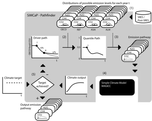
We will refer to the presented method as the ‘Equal Quantile Walk’ (EQW) ap-proach for reasons explained below. A concise overview on the consecutive steps of the EQW method is provided in Figure 1. The approach aims to distil a ‘ distri-bution of possible emission levels’ for each gas, each region and each year out of
a compilation of existing non-intervention and intervention scenarios in the litera-ture that use methods three and four above (see Figure 1 and Section 2). Once this distribution is derived, which is notably not a probability distribution (cf. Section 5.1.2), emissions pathways can be found, that are ‘comparably low’ or ‘comparably high’ for each gas. In this way the EQW method builds on the sophistication and detailed approaches that are inherent in existing intervention and non-intervention scenarios without making its own specific assumptions on different gases’ reduction potentials.
Here, the term ‘comparably low’ is defined as a set of emissions that are on the
same ‘quantile’ of their respective gas and region specific distributions. Hence, the approach is called ‘Equal Quantile Walk’ (cf. Figure 3 and Section 3.3). For exam-ple, thequantile path can, over time, be derived by prescribing one specific gas’s
emissions path in a particular region, such as fossil fuel CO2for the OECD region
(Section 3.2). The corresponding quantile path is then applied to all remaining
gases and regions and a global emissions pathway is obtained by aggregating over the world regions (Section 3.3). Consequently, EQW pathway emissions for one gas can go up over time, while emission of another gas go down, but an EQW pathway for a more ambitious climate target will be assumed to have lower emissions across all gases compared to an EQW pathway for a less ambitious climate target. Subse-quently, a simple climate model is used to find the corresponding profiles of global mean temperatures, sea levels and other climate indicators. Here we use the simple climate model MAGICC 4.1 (Wigley and Raper, 2001, 2002; Wigley, 2003a). This
I
II -x%
-y%
OECD REF ASIA ALM
Simple Climate Model MAGICC SRES / Post-SRES Target achieved?
-CO2 CO2 CO2 CO2 CO2 N2O CO2 CO2 CO2 CO2 CO2 N2O CH4 CO2 + SiMCaP - Pathfinder (1) I 0 0.5 1 (2) (3) (4) (5) CO2 CO2 CO2 CO2 CO2 N2O CO2 CO2 CO2 CO2 CO2 N2O CH4 CO2 Emission pathway Climate target Output emission pathway CO2 CO2 CO2 CO2 CO2 N2O CO2 CO2 CO2 CO2 CO2 N2O CH4 CO2 CO2 CO2 CO2 CO2 CO2 N2O CO2 CO2 CO2 CO2 CO2 N2O CH4 CO2 CO2 CO2 CO2 CO2 CO2 N2O CO2 CO2 CO2 CO2 CO2 N2O CH4 CO2 CO2 CO2 CO2 CO2 CO2 N2O CO2 CO2 CO2 CO2 CO2 N2O CH4 CO2 OECD f ossil C O2Driver path Quantile Path
Climate output
Distributions of possible emission levels for each year t
t t t t t t t t t t
Figure 1. The EQW method as implemented in SiMCaP’s ‘pathfinder’ module. (1) The ‘distributions of possible emission levels’ are distilled from a pool of existing scenarios for the 4 SRES world regions OECD, REF, ASIA and ALM.13(2) The common quantile path of the new emissions pathway
is derived by using a driver emission path, such as the one for fossil CO2 emissions in OECD countries. The driver path is here defined by sections of constant emission reductions (‘−x/y%’) and years at which the reduction rates change (‘I’ and ‘II’). (3) A global emissions pathway is obtained by assuming that – in the default case – the quantile path that corresponds to the driver path applies to all gases and regions. (4) Using the simple climate model MAGICC, the climate implications of the emissions pathway are computed. (5) Within SiMCaP’s iterative optimisation procedure, the quantile paths are optimised until the climate outputs and the prescribed climate target match sufficiently well.
is the model that was used for global-mean temperature and sea level projections in the IPCC TAR (see Cubasch et al., 2001 and Section 3.4 and Appendix A).
An iterative procedure is used to find emissions pathways that correspond to a predefined arbitrary climate target. This is implemented in the ‘EQW pathfinder’ module of the ‘Simple Model for Climate Policy Assessment’ (SiMCaP). More specifically, SiMCaP’s iterative procedure begins with a single ‘driver’ emission path (such as fossil CO2 in the OECD region) and then uses the ‘equal quantile’
assumption to define emissions for all other gases and regions. The driver path is then varied until the specified climate target is sufficiently well approximated using a least-squares goodness of fit indicator (see Figure 1). SiMCaP’s model
components and a set of derived EQW emissions pathways are available from the authors or at http://www.simcap.org.
3.1. DISTILLING A DISTRIBUTION OF POSSIBLE EMISSION LEVELS
In order to determine a possible range of different gases’ emission levels a set of scenarios is needed. Here, the 40 non-intervention IPCC emission scenarios from the Special Report on Emission Scenarios (Nakicenovic and Swart, 2000)2 are
used in combination with 14 Post-SRES stabilization scenarios from the same six modeling groups,3 as presented by Swart et al. (2002). This combined set of 54 scenarios is used in this study to derive the distributions of possible emission lev-els. The Post-SRES intervention scenarios are scenarios that stabilize atmospheric CO2 concentrations at levels between 450 ppm to 750 ppm. Most of the
Post-SRES scenarios only target fossil CO2explicitly, although lower non-CO2
emis-sions are often implied due to induced changes on all energy-related emisemis-sions. For halocarbons (CFCs, HCFCs and HFCs) and other halogenated compounds (PFCs, SF6), the post-SRES scenarios, however, provide no additional
informa-tion. Therefore, the A1, A2, B1 and B2 non-intervention IPCC SRES scenarios were supplemented with one intervention pathway in order to derive the distribu-tion of possible emission levels. Since most of the halocarbons and halogenated compounds can be reduced at comparatively low costs compared to other gases (cf. USEPA, 2003; Ottinger-Schaefer et al., submitted), the added intervention path-way assumes a smooth phase-out by 2075. Clearly, future applications of the EQW method can be based on an extended set of underlying multi-gas scenarios (such as EMF-21), thereby capturing the best available knowledge on multi-gas mitigation potentials.
The combined density distribution for the emission levels of the different gases has been derived by assuming a Gaussian smoothing window (kernel) around each of the 54 scenarios. The resulting non-parametric density distribution for a given year and gas can be viewed as a smoothed histogram of the data (see Figure 2). A narrow kernel would reveal higher details of the underlying data until every single scenario is portrayed as a spike–as in a high-resolution histogram. Wider kernels can also be used to some degree to interpolate and extrapolate information of the limited set of reduction scenarios into underrepresented areas within and outside the range of the scenarios. Thus, the chosen kernel width has to strike a balance between-on the one hand-allowing a smooth continuum of emission levels and the design of slightly lower emissions pathways and – on the other hand – appropriately reflect-ing the lower bound as well as the possibly asymmetric nature of the underlyreflect-ing data.
In this study, a medium width of the kernel is chosen-close to the optimum for estimating normal distributions (Bowman and Azzalini, 1997). For a limited number of cases a narrower kernel width was chosen, namely for the N2O related
0 1 2 3 4 5 6 7 (GtC)
0 50 100 150 200 250 (MtCH4)
a) OECD; Fossil CO2; 2050
b) OECD; CH4; 2100 narrow narrow medium medium wide wide densit y densit y
Figure 2. Derived non-parametric density distribution by applying smoothing kernels with default kernel width for this study (solid line ‘medium’), a wide kernel width (dashed line ‘wide’) and a narrow kernel width (dotted line ‘narrow’). See text for discussion.
distributions in order to better reflect the lower bound of the distribution. A narrower kernel for N2O guarantees a more appropriate reflection of the sharp lower bound
of the distribution of N2O emission levels, which is suggested by the pool of
existing SRES & post-SRES scenarios (see Figure 9c). The application of a wider kernel would have resulted in an extensive lapping of the derived non-parametric distribution into low emission levels that are not represented within the set of existing scenarios. The inclusion of a wider set of currently developed multi-gas scenarios might actually soften this seemingly hard lower bound for N2O emissions
in the future.4Furthermore, the distribution of possible emission levels might extend
into negative areas, which is, for most emissions, an implausible or impossible characteristic. Thus, derived distributions have been truncated at zero with the exception of land-use related net CO2emissions.
Land use CO2emissions, or rather CO2removal, have been bound at the lower
end according to the SRES scenario database literature range as presented in fig-ure SPM-2 of the Special Report on Emission Scenarios (Nakicenovic and Swart, 2000). Specifically, the applied lower bound ranges between−1.1 and −0.6 GtC/yr between 2020 and 2100. The maximum total uptake of carbon in the terrestrial biosphere from policies in this area over the coming centuries is assumed to ap-proximately restore the total amount of carbon lost from the terrestrial biosphere. Specifically, it was assumed that from 2100 to 2200, the lower bound for the land-use related CO2emission distribution smoothly returns to zero so that the accumulated
sequestration since 1990 does not exceed the deforestation related emissions be-tween 1850 and 1989, estimated to be 132 GtC5(Houghton, 1999; Houghton and
3.2. DERIVING THE QUANTILE PATH
For an EQW pathway, emissions of each gas in a given year and for a given region are assumed to correspond to the same quantile of the respective (gas-, year- and region-specific)distribution of possible emission levels. Depending on the climate
target and the timing of emission reductions, the annual quantiles might of course change over time (cf. inset (2) in Figure 1). It is possible to prescribe thequantile path directly. For example, aggregating emissions that correspond to the
time-constant 50% quantile path would result in the median pathway over the whole scenario data pool. In general, however, what we do is prescribe one of the gases’ emissions as ‘driver path’, for example the one for fossil CO2emissions in OECD
countries. The correspondingquantile path can then be applied to all other gases
in that region. If desired, the same quantile path may be applied to all regions. For a discussion on the validity of such an assumption of ‘equal quantiles’ the reader is referred to Section 5.1.1 with alternatives being briefly discussed in Section 5.1.7. Theoretically, one could for example also prescribe aggregate emissions as they are controlled under the Kyoto Protocol (Kyoto gases) and any consecutive treaties using 100-yr GWPs.14 Specifically, one could derive the corresponding
quantile path by projecting the prescribed aggregate emissions onto the distribution
of possible aggregate emission levels implied by the underlying scenarios. Such quantile paths, possibly regionally differentiated due to different commitments, could then be applied to all gases individually in the respective regions, provided a pool of standardized scenarios for the same regional disaggregation existed.
In this study, we have adopted a fairly conventional set of climate policy as-sumptions to derive the emissions pathways. One of the key agreed principles in the almost universally ratified United Nations Framework Convention on Climate Change (UNFCCC, Article 3.1) is that of “common but differentiated responsi-bilities and respective caparesponsi-bilities” which requires that “developed country Parties should take the lead in combating climate change”.1As a consequence, it is ap-propriate to allow the emission reductions in non-Annex I regions6 to lag behind
the driver. Furthermore, a constant reduction rate (exponential decline) of absolute OECD fossil CO2emissions has been assumed for ‘peaking’ scenarios after a
pre-defined ‘departure year’ from the baseline emission scenario (here assumed to be the median over all 54 IPCC scenarios). For ‘stabilization’ scenarios, the annual rate of reduction was allowed to change once in the future in order to lead to the desired stabilization level (see inset 2 within Figure 1). A constant annual emission reduction rate has been chosen for two reasons: (a) simplicity, and (b) because of the fact that such a path is among those that minimize the maximum of annual reductions rates needed to reach a certain climate target.
Up to the predefineddeparture year, e.g. 2010, emissions follow the median
scenario (quantile 0.5; cf. Figure 3). The departure year can differ from region to region and indeed, as noted above, this is required by the UNFCCC and codified further in the principles, structure and specific obligations in the Kyoto Protocol.
0 0.5 1 100 101 102 103 104 OECD Emissions (MtC O2 eq) 0 0.5 1 0 0.5 1 Fossil CO2 CH4 N2O CF4 C2F6 HFC-134a SF6 Quantile Quantile Quantile Fossil CO2 CH4 N2O CF4 C2F6 HFC-125 HFC-134a HFC-143a HFC-227ea HFC-245ca SF6 Fossil CO2 CH4 N2O CF4 C2F6 HFC-125 HFC-134a HFC-143a HFC-227ea HFC-245ca SF6
Year 2000 Year 2050 Year 2100
Figure 3. The derived distributions of possible emission levels displayed as (inverse) cumulative distribution functions for OECD countries in the years 2000 (right), 2050 (middle) and 2100 (left). The nearly horizontal lines for the year 2000 (left panel) illustrate that all 54 underlying scenarios share approximately the same emission level assumptions for the year 2000 (basically because these scenarios are standardized). In later years, here shown for 2050 and 2100, the scenarios’ projected emissions diverge, so that the lower percentile (left side of each panel) corresponds to lower emissions compared to the upper percentile (right side of each panel) of the emission distributions. Thus, the slope of cumulative emission distribution curves goes from lower-left to upper-right. New mitigation pathways are now constructed by assuming a set of emissions for each year that corresponds to the same quantile (black triangles) in a respective year. These quantiles can for example be chosen so that a prescribed emission path for fossil CO2is matched. The non-fossil CO2emissions are then chosen
according to the same quantile (see dots on dashed vertical lines). The same procedure is applied to other non-OECD world regions by using either the same or different quantile path (see text). For this illustrative figure (but not for any of the underlying calculations within the EQW method), all emissions have been converted to Mt CO2-equivalent using 100-yr GWPs.14Note the logarithmic
vertical scale, which causes zero and negative emissions not being displayed.
Here non-Annex I countries are assumed to diverge from the baseline scenario a bit later (2015) than Annex-I countries (2010) and follow aquantile path that
corresponds to a hypothetically delayed departure of fossil fuel CO2emissions in
OECD countries.
Generally, it should be noted that there could be a difference between actual emissions and the assumed emission limitations in each region to the extent that emissions are traded between developed and developing countries.
3.3. FINDING EMISSIONS PATHWAYS
Once the non-parametricdistributions of possible emission levels (Section 3.1) are
defined and thequantile paths (3.2) prescribed, multi-gas emissions pathways for
any possible climate target can be derived. For any specific year, the emission levels of each greenhouse gas and aerosol for different regions are selected according to a specific single quantile for the particular year and region. This will result in a set of emissions that is ‘comparably low’ or ‘high’ in relation to the underlying pool of existing emission scenarios (see Figure 3). As a final step a smoothing spline algorithm has been applied to the individual gases pathways other than the driver path, restricted to the years after the regions’ departure year from the baseline scenario.
3.4. THE CLIMATE MODEL
All major greenhouse gases and aerosols are inputs into the climate model, namely carbon dioxide (CO2), methane (CH4), nitrous oxide (N2O), the two most relevant
perfluorocarbons (CF4, C2F6), and five most relevant hydrofluorocarbons
(HFC-125, HFC-134a, HFC-143a, HFC-227ea, HFC-245ca), sulphur hexafluoride (SF6),
sulphate aerosols (SO2), nitrogen oxides (NOx), non-methane volatile organic
com-pounds (VOC), and carbon monoxide (CO). Emissions of these gases are calculated for the different climate targets using the EQW method. Thus, these emissions were varied according to the stringency of the climate target. For the limited number of re-maining human-induced forcing agents, the assumed emissions follow either a ‘one size fits all’ or ‘scaling’ approach, due to the lack of data within the pool of SRES
and Post-SRES scenarios. Specifically, the forcing due to substances controlled by the Montreal Protocol is assumed to be the same for all emissions pathways. Similarly, emissions of other halocarbons and halogenated compounds aside from those eight explicitly modeled are assumed to return linearly to zero over 2100 to 2200 (‘one size fits all’). The combined forcing due to fossil organic carbon and
black organic carbon was scaled with SO2emissions after 1990 (‘scaling’), as in
the IPCC TAR global-mean temperature calculations.
A brief description of the default assumptions made in regard to the employed simple climate model MAGICC and natural forcings are given in the Appendix.
4. ‘Equal Quantile Walk’ Emissions Pathways
The following section presents some results in order to highlight some of the key characteristics of the EQW method. First, we compare the results of the EQW method with previous CO2 concentration stabilization pathways. It is shown that
stabilization level, which is the result of EQW pathways taking into account the non-CO2mitigation potentials to the extent that they are included in the underlying
multi-gas scenarios. Second, we examine two sets of peaking pathways, where the global mean radiative forcing peaks and hence where concentrations do not necessarily stabilize (not as soon as under CO2 stabilization profiles at least). In
principle, these may be useful in examining emissions pathways corresponding to climate policy targets that recognize that it may be necessary to lower peak temperatures in the long term in order to take account of–for example–concerns over ice sheet stability (Oppenheimer, 1998; Hansen, 2003; Oppenheimer and Alley, 2004). Provided one makes specific assumptions on the most important climate parameters, such as climate sensitivity, one could also derive temperature (rate) limited pathways (not shown in this study).
4.1. COMPARISON WITH PREVIOUS PATHWAYS
This section compares EQW multi-gas emissions pathways with emissions of the S and WRE CO2stabilization profiles. In order to allow a comparison between these
emissions pathways, sample ‘EQW’ emissions pathways were designed to reach CO2stabilization at 350 to 750 ppm. After the default departure years (2010 for
Annex I regions and 2015 for non-Annex I), the quantile path corresponds to a rate of reduction of OECD fossil CO2emissions between−5.2% and −0.5% annually
depending on the stabilization level. These annual emission reductions are adjusted at a point in the future (derived in the optimization procedure) in order to allow CO2concentrations to stay at the prescribed stabilization levels (see Table II).
While fossil CO2 emissions between WRE and these sample EQW pathways
converge in the long-term, the near and medium-term fossil CO2emissions differ
(see Figure 4). For the lower stabilization levels, the assumptions chosen here for the EQW pathways lead to slightly higher fossil CO2 emissions than the WRE
pathways, which is mainly due to the fact that the land-use related CO2emissions
are substantially lower under the EQW than under WRE. For the same reason, cumulative fossil CO2 emissions are slightly higher for the EQW pathways than
for the corresponding WRE pathways (not shown in figures). For the less stringent profiles, namely stabilization levels between 550 and 750 ppm, the EQW assump-tions lead to fossil CO2emissions that are lower in the near term, but decline more
slowly and are higher in the 22nd century and beyond. The main reason for this difference might be of a methodological nature rather than founded on differing explicit assumptions on ‘early action’ vs. ‘delayed response’. As for the original S profiles and many recent stabilization profiles (Eickhout et al., 2003), the WRE profiles were defined as smoothly varying CO2 concentration curves using Pad´e
approximants (cf. Enting et al., 1994) and emissions were determined by inverse calculations. In contrast to this ‘top-down’ approach, the EQW method can be cat-egorized as a ‘bottom-up’ approach in the transient period up to CO2stabilization,
T ABLE II Reduction rates for OECD fossil CO 2 (driver paths ), W orld fossil CO 2 and W orld aggre gated K yoto gases (6-GHGs) with and without ‘Other CO 2 ’ that are compatible with reaching CO 2 stabilisation le v els from 350 to 750 ppm according to the EQW method. After the departure years (2010/2015 for Anne x-I/ non-Anne x I), OECD fossil CO 2 emissions are assumed to decrease at a constant rate (‘Reduction rate I’). From the ‘adjustment year ’ onw ards, the annual emission reduction rate is reduced in order to stabilize CO 2 concentrations (‘Reduction rate II’). The three presented parameter v alues, reduction rate I and II and the adjustment year , are optimal in the sense, that the resulting CO 2 concentration profiles best match the prescribed stabilization le v els under a least-squares goodness-of-fit indicator . Other sources’ and gases’ emissions follo w the same quantile path (see Section 3.3) resulting in v ariable w orldwide reduction rates for fossil CO 2 and aggre gated emissions (using 100-yr GWPs) o v er time. W orld F ossil W orld 6-GHGs W orld 6-GHGs CO 2 excl. ‘Other CO 2 ’ incl. ‘Other CO 2 ’ OECD F ossil CO 2 CO 2 Range reduction Range reduction Range reduction stabilization Reduction rate Adjustment Reduction rate rates 2020–2100 rates 2020–2100 rates 2020–2100 le v el (ppm) I (%/year) year II (%/year) (%/year) (%/year) (%/year) 350 − 5.17 2120 0.00 − 1.05 to − 4.64 − 0.61 to − 3.24 − 0.28 to − 5.19 450 − 2.18 2070 − 0.74 − 0.62 to − 1.31 − 0.65 to − 0.93 − 0.71 to − 1.57 550 − 0.93 2211 − 0.38 + 0.62 to − 1.01 + 0.40 to − 0.82 + 0.03 to − 1.12 650 − 0.63 2327 − 0.01 + 0.86 to − 0.67 + 0.66 to − 0.59 + 0.40 to − 0.77 750 − 0.46 2379 0.00 + 0.98 to − 0.48 + 0.80 to − 0.44 + 0.59 to − 0.55
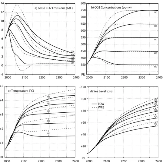
PIL +1 +2 +3 +4 +5 2000 2100 2200 2300 2400 -2 0 2 4 6 8 10 12 14 2000 2100 2200 2300 2400 PIL 350 400 450 500 550 600 650 700 750 800 b) CO2 Concentrations (ppmv) c) Temperature (˚C)
a) Fossil CO2 Emissions (GtC)
d) Sea Level (cm) WRE 2000 2100 2200 2300 2400 2000 2100 2200 2300 2400 PIL +20 +40 +60 +80 +100 +120 750 650 550 350 450 750 650 550 350 450 750 650 550 350 450 750 650 550 350 450 EQW
Figure 4. Comparison of WRE profiles (dashed) with EQW profiles (solid). (a) Fossil CO2pathways
differ (see text) for the (b) prescribed CO2 stabilization levels at 350, 450, 550, 650 and 750 ppm.
(c) Global mean surface temperature increases above pre-industrial levels (‘PIL’) are lower for the EQW profiles for any CO2stabilization (c) due to lower non-CO2emissions. Correspondingly, sea
level increases are lower for EQW profiles (d). As in the IPCC TAR (cf. figure 9.16 in Cubasch et al., 2001), the WRE CO2emissions pathways are here combined with non-CO2emissions according to
the IPCC SRES A1B-AIM scenario (dashed lines).
since the profile towards CO2stabilization is prescribed by multiple constraints on
the fossil CO2emissions rather than on CO2concentrations themselves.
Under the most stringent of the analyzed CO2concentration targets, stabilization
at 350 ppm, near term fossil CO2 emissions depart, slightly delayed, from the
baseline scenario in comparison to the WRE350 pathway, which assumes a global departure in 2000 (cf. Figure 4). Compared to the S-profiles, this difference (for all stabilization levels) is even larger as the S profiles assume an early start of
emission reductions in the 1990s and a smoother path thereafter, which already seems unachievable today, due to recent emissions increases.
A comparison including non-CO2 gases can be done using the WRE profiles
as they are presented in the IPCC TAR (see figure 9.16 in Cubasch et al., 2001). There, the effects for the WRE CO2stabilization profiles are computed by assuming
non-CO2 gas emissions according to the A1B-AIM scenario (see Figure 4 and
Figure 5. For the comparison, it is thus important to keep in mind that the EQW pathways are not compared to the WRE CO2 profiles per se, but to the WRE
pathways in combination with this specific assumption for non-CO2emissions.
The EQW method chooses non-CO2emissions on the basis of the CO2quantile,
which for all analyzed CO2stabilization profiles implies that it chooses emissions
significantly below the A1B-AIM levels–as also the fossil CO2emissions are below
those of the A1B-AIM scenario. Mainly due to these lower non-CO2emissions, the
radiative forcing implications related to EQW pathways are significantly reduced for the same CO2 stabilization level when compared to WRE pathways, i.e. for
stabilization at 450 ppm (see Figure 5). Partially offsetting this ‘cooling’ effect is the reduced negative forcing due to decreased aerosol emissions. The negative forcing from aerosols can be significant (cf. dark area below zero in Figure 5) and can mask some positive forcing due to CO2 and other greenhouse gases. In the
year 2000, this masking is likely to be about equivalent to the forcing due to CO2
alone (the upper boundary of the “CO2” area is near the zero line in Figure 5).
However, note that large uncertainties persist in regard to the direct and indirect radiative forcing of aerosols (see e.g. Anderson et al., 2003).7The total radiative
forcing for the WRE450 scenario in 2400 is ca. 3.9 W/m2and around 3 W/m2for the EQW-S450C.
Owing to the effect on radiative forcing, the lowered non-CO2emissions that
result from the EQW method lead to less pronounced global mean temperature increases in comparison to the WRE CO2 stabilization profiles in combination
with the A1B-AIM non-CO2emissions. For the same CO2stabilisation levels, the
corresponding temperatures are about 0.5◦C cooler by the year 2400 (assuming a climate sensitivity of approximately 2.8◦C by computing the ensemble mean over 7 AOGCMs-see Appendix A). Consequently, the sea level rise is also slightly reduced when assuming the EQW pathways (cf. Figure 4).
4.2. RADIATIVE FORCING(CO2EQUIVALENT)PEAKING PROFILES
A variety of climate targets can be chosen to derive emissions pathways with the EQW method. In this section, two sets of multi-gas emissions pathways are chosen so that the corresponding radiative forcing peaks between approximately 2.6 and 4.5 W/m2with respect to pre-industrial levels. The CO2equivalent peaking
concentrations are 475 to 650 ppm (see Figure 6). No time-constraint is placed on the attainment of the peak forcing.
1700 1800 1900 2000 2100 2200 2300 2400 -2 -1 0 1 2 3 4 SO4DIR SO4IND BIOAER
CO2
CH4 N2O HALOtot TROPOZ FOC+FBC EQW-S450C -1 0 1 2 3 4 5 R adiativ e F or cing ( W/m 2) R adiativ e F or cing ( W/m 2) SO4DIR SO4IND BIOAERCO2
CH4 N2O HALOtot TROPOZ FOC+FBC WRE450(with non-CO2 acc. to SRES A1B-AIM)
Figure 5. Aggregated radiative forcing as a result of the WRE emissions pathway (upper graph) and the EQW pathway (lower graph) for stabilization of CO2concentrations at 450 ppm. Since the ‘EQW’
multi-gas pathways take into account reductions of non-CO2gases, the positive radiative forcing due
to CH4, N2O, tropospheric ozone (‘TROPOZ’), halocarbons and other halogenated compounds minus
the cooling effect due to stratospheric ozone depletion (‘HALOtot’) as well as the negative radiative forcing due to sulphate aerosols (indirect ‘SO4IND’ and direct ‘SO4DIR’) and biomass burning related aerosols (‘BIOAER’) is substantially reduced. The combined warming and cooling due to fossil fuel related organic & black carbon emissions (‘FOC+FBC’) is scaled towards SO2emissions
(see text).
The first set ‘A’ of derived EQW peaking pathways assumes a fixed departure year, but variable rates of emission reductions thereafter. The second set ‘B’ holds the reduction rates of the driver emission path constant, but assumes varying de-parture years. Specifically, the peaking pathways ‘A’ assume a dede-parture from the median emission scenario in 2010 for Annex I countries (IPCC SRES regions REF
& OECD13and a departure in 2015 for non-Annex I countries (ASIA & ALM). OECD fossil CO2 emissions, the driver emission path, are assumed to decline at
a constant rate, which differs between the individual pathways ‘A’, after the fixed departure year. The second set ‘B’ of peaking pathways assumes a departure year from the median emission scenario between 2010 and 2050 for Annex I countries (5 years later for non-Annex I countries), and a 3% decline of OECD fossil CO2
driver path emissions. As highlighted in the method section, emissions in non-OECD regions and from non-fossil CO2sources are assumed to follow thequantile path corresponding to the preset driver path (see Figure 6, Section 3.2 and 3.3).
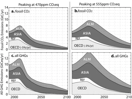
For the derived emissions pathways that peak between 470 and 555 ppm CO2eq,
global fossil CO2emissions are between 46% to 113 % of 1990 emission levels in
2050 (see Table III) and 11% to 33% in 2100, depending on the peaking target. In parallel to the greenhouse gas emissions, the EQW method derives aerosol and ozone precursor emissions that are ‘comparably low’ in regard to the
underly-ing set of SRES/Post-SRES scenarios. Thus, despite the fact that sulphate aerosol precursor emissions (SOx) have a cooling effect, SOx emissions are assumed to
decline sharply for the more stringent climate targets (see Table III). The linkage between SOx and CO2 emissions is also seen in mitigation scenarios from
cou-pled socio-economic, technological model studies and is partially due to the fact that both stem from a common source, namely fossil fuel combustion (see as well Section 5.1.1). Another reason is that mitigation scenarios represent future worlds which inherently include environmental policies in both developed and developing countries-where the abatement of acid deposition and local air pollution has usually even higher priority than greenhouse gas abatement.
Depending on the shape of the emissions pathways (e.g. set A or B), and de-pending on the peak level between 470 and 650 ppm CO2eq, radiative forcing peaks
between 2025 and 2100. After peaking, radiative forcing (CO2equivalence
concen-trations) stays significantly above pre-industrial levels for several centuries. This is ←−−−−−−−−−−−−−−−−−−−−−−−−−−−−−−−−−−−−−−−−−−−−−−−−−−−−−−−−−
Figure 6. Two sets of multi-gas pathways derived with the EQW method. The two sets are distinct in so far as set A assumes a fixed departure year from the median emission path (2010) and a different reduction rate thereafter (−7% to 0%) (A.1). The pathways of set B assume a fixed reduction rate for OECD fossil CO2emissions (−3%/yr), but variable departure years. Emissions of other gases and in
other regions follow the corresponding quantile paths (see text). For illustrative purposes, the GWP-weighted sum of greenhouse gas emission is shown in panels A.2 and B.2. Using a simple climate model, the radiative forcing implications of the multi-gas emissions pathways can be computed, here shown as CO2 equivalent concentrations with black dots indicating the peak values (A.3 and
B.3). The temperature implications are computed probabilistically for each peaking pathway using a range of different climate sensitivity pdfs (see text). In this way, one can illustrate the probability of overshooting a certain temperature threshold (here 2◦C above pre-industrial) under such peaking pathways given different climate sensitivity probability distributions (dashed lines in darker shaded area of A.4 and B.4). Lighter shaded areas depict the probability of overshooting 2◦C in equilibrium in case that concentrations were stabilized and not decreased after the peak. The full set of emission data is available at http://www.simcap.org.
TABLE III
Specifications (I), emission implications (II) and probabilities of overshooting 2◦C (III) for three radiative forcing peaking pathways (cf. Figure 6). Departure years and annual OECD fossil CO2emission reductions (‘driver path’) were prescribed. For illustrative purposes only,
greenhouse gas emissions (CO2, CH4, N2O, HFCs, PFCs, and SF6) were aggregated using
100-year GWPs14including and excluding landuse related CO
2emissions (‘other CO2’). The
maximum CO2equivalence concentration (radiative forcing) is shown and its associated
prob-ability of overshooting 2◦C global mean temperature rise above pre-industrial for a range of different climate sensitivity probability density function estimates (see text). The probability of overshooting is clearly lower for the peaking pathways, where concentrations drop after reach-ing the peak level, in comparison to hypothetical stabilization pathways, where concentrations are stabilized at the peak.
Peaking Peaking Peaking
pathway 1 pathway 2 pathway 3 I. Specifications
Set of pathway A A/B B
Departure years (Annex I/Non-Annex I) 2010/15 2010/15 2020/25
Driver path OECD fossil CO2reduction −5%/yr −3%/yr −3%/yr
II. Emission implications
Emissions (1990 level) 2050 Emissions relative to 1990
Fossil CO2(5.98 GtC) 46% 80% 113%
CH4(309 Mt) 77% 94% 112%
N2O (6.67 TgN) 68% 76% 81%
GHG excl. other CO2(8.72 GtCeq) 55% 82% 110%
GHG incl. other CO2(9.82 GtCeq) 41% 65% 90%
SOx(70.88 TgS) 4% 13% 26%
III. Peak concentration and probability of overshooting
Peak concentration CO2eq ppm (radiative 470 (2.80) 503 (3.17) 555 (3.70)
forcing W/m2)18
Probability>2◦C (peaking) 5–60% 25–77% 48–96%
Probability>2◦C (stabilisation) 35–88% 49–96% 69–100%
mainly due to the slow redistribution processes for CO2between the atmospheric,
oceanic and abyssal sediment carbon pools.
The temperature response of the climate system is largely dependent upon its cli-mate sensitivity, which is rather uncertain. A range of recent studies have attempted to quantify this uncertainty in terms of probability density functions (PDFs) (see e.g. Andronova and Schlesinger, 2001; Forest et al., 2002; Gregory et al., 2002; Knutti et al., 2003; Murphy et al., 2004). These studies are used here to compute each emissions pathway’s probabilistic climate implications by running the simple climate model with an array of climate sensitivities, weighted by their respective probabilities according to particular climate sensitivity PDFs. The probabilistic
temperature implications of the radiative forcing peaking pathway sets can then be shown in terms of their probability of overshooting a certain temperature threshold, here chosen as 2◦C above pre-industrial levels (see it Figure 6). The faster the radia-tive forcing drops to lower levels after the peak, the less time there is for the climate system to reach equilibrium warming. Thus, for peak levels of 550 ppm CO2eq and
above, the peaking pathways B involve slightly lower probabilities of overshooting a 2◦C temperature thresholds, as their concentrations decrease slightly faster than for the higher peaking pathways of set A. The probability of overshooting 2◦C would obviously be higher for both sets, if radiative forcing were not decreasing after peaking, but stabilized at its peak value, as depicted by the lighter shaded areas in Figure 6 A.4 and B.4 (Azar and Rodhe, 1997; Hare and Meinshausen, 2004; Meinshausen, 2005).
In summary, it has been shown that the EQW method can provide a useful tool to obtain a large numbers of multi-gas pathways to analyze research questions in a probabilistic setting. Furthermore, the results suggest that if radiative forcing is not peaked at or below 475 ppm CO2eq (∼2.8 W/m2) with declining concentrations
thereafter, it seems that an overshooting of 2◦C can not be excluded with reasonable confidence levels (see Figure 6).
5. Discussion and Limitations
The following section discusses some of the potential limitations, namely those related to the EQW method itself (Section 5.1), and those related to the underlying pool of scenarios (Section 5.2). In addition, the use of a simple climate model implies some limitations briefly mentioned in Appendix A.
5.1. DISCUSSION OF AND POSSIBLE LIMITATIONS ARISING FROM THE METHOD ITSELF
The following section briefly discusses several issues that are directly related to the proposed EQW method: namely the assumption of unity rank correlations (5.1.1); the question, whether the individual underlying scenarios are assumed to have a certain probability (5.1.2); regional emission outcomes (5.1.4); the baseline (in-)dependency (5.1.5); land-use change related emissions and their possible political interpretations (5.1.5); alternative gas-to-gas and timing strategies (5.1.7); and the probabilistic framework (5.1.8).
5.1.1. Unity Rank Correlation
New emissions pathways produced with the EQW method will rank equally across all gases in a specific region for a specific year. In other words, an emissions pathway for a less stringent climate target (e.g. peaking at 550 ppm CO2eq) has
higher emissions for all gases and all regions compared to an emissions pathway for a less stringent climate target (e.g. 475 ppm CO2eq).
Note that this inbuilt unity rank correlation assumption of the EQW method does not necessarily lead to positive absolute correlations between different gases’ or regions’ emissions. In other words, for a particular EQW mitigation pathway, emissions of one gas, e.g. CO2 in Asia, might still be increasing in a particular
year, while emissions of another gas, e.g. methane in OECD, are already decreas-ing dependdecreas-ing on the emission distributions in the underlydecreas-ing pool of emission scenarios.
The unity rank correlation could be an advantage of the EQW approach. How-ever, it could also be a limitation in the presence of negative rank correlations for emissions: for example, if fossil fuel emissions were largely reduced due to a replacement with biomass, a negative correlation might arise between fossil fuel CO2and biomass-burning related aerosol emissions, such as SOx, NOx etc. Thus,
if fossil fuel CO2emissions decrease, some aerosol emissions might increase. NOx
and N2O emission changes may be negatively correlated up to a certain degree as
well. Coupled socio-economic, technological, and land use models, such as those used for creating the SRES and Post-SRES scenarios, are generally able to account for these underlying anti-correlation effects. Thus, the following analysis assumes that an analysis of the SRES and Post-SRES scenarios can provide insights about real world dynamics in regard to whether inherent process based anti-correlations of emissions are so dominant, that the unity rank correlation assumption at given aggregation levels would be invalidated.
The question is, therefore, whether any negative rank correlations are apparent at the aggregation level considered here, namely the 4 SRES world regions. For the pool of existing SRES and Post-SRES scenarios that are used, no negative rank correlations between fossil fuel CO2and any other gases’ emissions are apparent
at this stage of aggregation by sources and regions (see Figure 7 and Appendix B). The rank correlation between fossil fuel CO2 and ‘Other CO2’ or ‘N2O total’ is
basically zero or rather small, while rank correlations with other gases are positive, especially for the ASIA and ALM region.
Between fossil fuel CO2 and the land-use and agriculture dominated ‘Other
CO2’ and ‘N2O’ emissions, there is little or no rank correlation. In other words, in
the underlying SRES and post SRES data set, the sources of these emissions are largely unrelated. The primary reason for this is that ‘Other CO2’ sources are at
present dominated by tropical deforestation (Fearnside, 2000). Another reason why existing scenarios with low fossil fuel CO2emissions do not necessarily correspond
to large reductions in deforestation emissions or large net sequestration appears to be that some modeling groups assume different policy mixes or different root causes of deforestation–potentially out of reach for climate policies.
In summary, the validity of the EQW approach is not limited as long as it is only applied at aggregation levels, where negative rank correlations are generally not evident, as is the case in this study. The fact that there are inherent, process
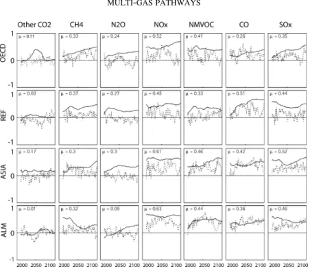
Figure 7. Rank correlations within the pool of existing SRES/Post-SRES scenarios between fossil fuel CO2emissions and other greenhouse gas emissions and aerosols (columns) for the 4 SRES World
regions (rows). The Kendall rank correlation (solid line), its mean from 2010 to 2100 (μ) and the Spearman rank correlation (dotted lines) are given (see Appendix B).
based anti-correlations of certain emissions at local or more subsource-specific level(s), does not invalidate this unity rank correlation assumption, as long as these underlying anti-correlations are not dominant.
The differing population assumptions of the underlying scenarios might appear to be, at first sight, a reason for the positively rank correlated emissions across different gases. A scenario that assumes high population growth is likely to predict high human-induced emissions across all gases. However, a closer look at per-capita (instead of absolute) emissions shows that differing population assumptions are not the reason for the positively rank correlated emission levels nor the large variation of absolute emissions. Rank correlations across the different gases on a per-capita basis (a) are generally non-negative and (b) are not uniformly lower or higher across all regions and gases than do rank correlations that are based on absolute emissions. On average, these per capita rank correlations are only marginally lower than rank correlations based on absolute emissions. Specifically, the change of the mean Kendall rank correlation index over 2010 to 2100 is insignificantly different from zero (−0.008) when averaged over all gases. Maximal changes are +0.07 and−0.11 for some gases (standard deviation of 0.043), if per-capita emissions are analyzed instead of absolute emissions (cf. Figure 7).
Given the absence of negatively rank correlated emissions, the seeming dis-advantage of the EQW approach, namely that it assumes unity rank correlation between fossil CO2 emissions and those of other gases, might actually be an
ad-vantage. Since the EQW approach is primarily designed to create new families ofintervention pathways, correlating reduction efforts between otherwise
uncor-related greenhouse gas sources might be a sensible characteristic. In other words, for those sources that are not correlated with fossil fuel CO2 emissions, namely
land-use dominated and agricultural emissions, the EQW approach suggests that a climate-policy-mix might tackle these sources in parallel to tackling fossil fuel emissions. Given that some policy options are available to reduce emissions in the land-use sector (see e.g. Pretty et al., 2002; see e.g. Carvalho et al., 2004)8it would seem very likely that the more a reduction effort is put into reducing fossil fuel related emissions, the more a parallel reduction effort will be put into reducing land-use related emissions as well.
5.1.2. Assuming a Certain Probability of Underlying Scenarios?
The application of some statistical tools within the EQW method assumes equal validity of each of the 54 scenarios within the underlying pool. This assumption, however, does not affect the outcome. As the following results show, the EQW method is rather robust to the relative ‘probability’ (weighting) within the scenario pool. Thus, the EQW method is largely independent of the assumed likelihood of single scenarios.
The sensitivity of the EQW method to different weightings of the underlying scenarios has been analyzed as follows. Four sensitivity runs have been performed. In each of them, members of one of the four IPCC scenarios families A1, A2, B1 and B2 have been multiplied three times. In effect, the original 54 plus the multiplied scenarios were then analyzed to derive the ‘distributions of possible emission levels’, as outlined above (3.1). Keeping other parts of the EQW method the
same, intervention pathways were derived for global-mean temperature peaking at 2◦C above the pre-industrial level. The results show that the pathways’ sensitivities to the weighting are rather small. Obviously, if a scenario’s frequency or weight-factor is changed, slightly different emissions pathways will result, since basically all scenarios differ with respect to relative gas and regional shares (see Table IV).
Obviously, assuming a different set of scenarios altogether in order to derive the
distribution of possible emission levels might change the outcome considerably.
It should be kept in mind that the EQW method is not designed to determine how likely it might be that future emissions will be below a certain level. Similar to the medians calculated by Nakicenovic et al. (1998) for the IPCC database, the derived ‘distributions of possible emission levels’ are by no means probability estimations
(cf. e.g. Grubler and Nakicenovic, 2001). If, however, one would have a set of scenarios with a well defined likelihood for each of them, then more far reaching conclusions could be drawn instead of designing normative scenarios, as is done here.
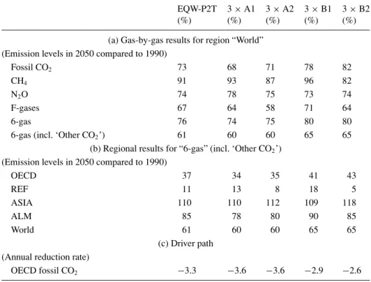
TABLE IV
Sensitivity analysis with respect to the underlying SRES scenario family frequencies. The common climate target ‘peaking below 2◦C’ is prescribed for and met by all 5 pathways assuming a climate sensitivity of 2.8◦C (7 AOGCM ensemble mean). Whereas the first pathway (EQW-P2T) was derived by using the underlying data pool of 54 unique scenarios, the four sensitivity pathways were derived by multiplying the frequency of A1, A2, B1 or B2 scenario family members three times (3× A1 to
3× B2). Shown are the emission levels in 2050 compared to 1990 levels for different gases (a) and
regions (b) and the annual reduction rate for OECD fossil CO2emissions (c)
EQW-P2T 3× A1 3 × A2 3 × B1 3 × B2
(%) (%) (%) (%) (%)
(a) Gas-by-gas results for region “World” (Emission levels in 2050 compared to 1990)
Fossil CO2 73 68 71 78 82
CH4 91 93 87 96 82
N2O 74 78 75 73 74
F-gases 67 64 58 71 64
6-gas 76 74 75 80 80
6-gas (incl. ‘Other CO2’) 61 60 60 65 65
(b) Regional results for “6-gas” (incl. ‘Other CO2’)
(Emission levels in 2050 compared to 1990)
OECD 37 34 35 41 43 REF 11 13 8 18 5 ASIA 110 110 112 109 118 ALM 85 78 80 90 85 World 61 60 60 65 65 (c) Driver path (Annual reduction rate)
OECD fossil CO2 −3.3 −3.6 −3.6 −2.9 −2.6
5.1.3. Sensitivity to Lower Range Scenarios
If the EQW method produces a new emissions pathway near to or slightly outside the range of existing scenarios, there is a high sensitivity to scenarios in the underlying data base that are at the edge of the existing distribution. Certain measures can and are applied to limit this sensitivity, and its undesired effects, by (a) using an appropriate kernel-width to derive the ‘distribution of possible emission levels’ (see Section 3.1), (b) enlarging the pool of underlying scenarios by explicit intervention scenarios at the lower edge of the distribution, namely by the inclusion of Post-SRES stabilization scenarios, while at the same time (c) restricting the pool to scenarios of widely accepted modeling groups with integrated and detailed models.
Clearly, entering ‘unexplored’ terrain with this approach is only a second best option in the absence of fully developed scenarios for the more stringent climate targets. Ideally, the EQW method would be applied on a large pool of scenarios
including those with the most stringent climate targets. Such fully developed mit-igation scenarios might be increasingly available in the future. For example, new MESSAGE and IMAGE model runs (Nakicenovic and Riahi, 2003; van Vuuren et al., 2003) and forthcoming multi-gas scenarios developed within the Energy Modeling Forum EMF-21 (see e.g. de la Chesnaye, 2003) could build the basis of updated EQW pathways.
5.1.4. Regional Emissions & Future Commitment Allocations
Geo-political realities, the historic responsibility of different regions, their ability to pay, capability to reduce emissions, vulnerability to impacts as well as other fairness and equity criteria will inform the global framework for the future differentiation of reduction commitments. Thus, splitting up a global emissions pathway and choosing a commitment differentiation is not solely a scientific or economic issue, but rather a (sensitive) political one.
Regionally different emission paths result from the application of the EQW method to the 4 SRES regions. This is a direct consequence of the regional emission shares within the pool of underlying SRES / Post-SRES scenarios as well as possibly regionally differentiateddeparture years from the median (see Section 3.2). Thus,
the EQW method is not, in itself, an emission allocation approach based on explicit differentiation criteria. The method captures the spectrum of allocations in the pool of underlying existing scenarios and allows for some flexibility by setting regionally differentiated departure years for example.
Under default assumptions, the derived emissions pathways entail an increasing share of non-Annex I emissions independent of the climate target (Figure 8). This is in accordance with many of the approaches for the differentiation of future commitments (den Elzen, 2002; H¨ohne et al., 2003). Nevertheless, a sensitivity analysis with different climate parameters, departure years and possibly different quantile paths for different regions allows making important contributions in the discussion on future commitments. In addition, EQW pathways can be used as input for detailed emission allocation analysis tools, such as FAIR (den Elzen and Lucas, 2005), in order to obtain assessments of future climate regime proposals that are consistent with certain climate targets.
5.1.5. Baseline Independency & Absence of Socio-Economic Paths
In line with the most popular previous mitigation pathways, the derived pathways do not attempt to reflect a certain economic development pathway. The socio-economic characteristics of a future world can hardly be derived by walking along certain quantiles of the distributions of GDP development, productivity, fertility, etc. As pointed out by Grubler and Nakicenovic (2001): “Socioeconomic variables and their alternative future development paths cannot be combined at will and are not freely interchangeable because of their interdependencies. One should not, for example, create a scenario combining low fertility with high infant mortality, or zero economic growth with rapid technological change and productivity growth – since