HAL Id: hal-03233662
https://hal.archives-ouvertes.fr/hal-03233662
Submitted on 26 May 2021
HAL is a multi-disciplinary open access
archive for the deposit and dissemination of
sci-entific research documents, whether they are
pub-lished or not. The documents may come from
teaching and research institutions in France or
abroad, or from public or private research centers.
L’archive ouverte pluridisciplinaire HAL, est
destinée au dépôt et à la diffusion de documents
scientifiques de niveau recherche, publiés ou non,
émanant des établissements d’enseignement et de
recherche français ou étrangers, des laboratoires
publics ou privés.
Data assimilation for urban noise maps generated by a
meta- model
Antoine Lesieur, Vivien Mallet, Pierre Aumond, Arnaud Can
To cite this version:
Antoine Lesieur, Vivien Mallet, Pierre Aumond, Arnaud Can. Data assimilation for urban noise maps
generated by a meta- model. Forum Acusticum 2021, Dec 2020, Lyon / Virtual, France. pp.697-698,
�10.48465/fa.2020.0389�. �hal-03233662�
DATA ASSIMILATION FOR URBAN NOISE MAPS GENERATED BY A
META-MODEL
Antoine Lesieur
1Vivien Mallet
1Pierre Aumond
2Arnaud Can
21
INRIA, LJLL, Sorbonne Universit´e, F-75012 Paris, France
2
UMRAE, Univ Gustave Eiffel, IFSTTAR, CEREMA, F-44344 Bouguenais, France
[email protected], [email protected],[email protected], [email protected]
1. INTRODUCTION
A regulatory noise map is a 2D representation of the equiv-alent average noise level field over an urban area. In methods such as CNOSSOS-EU, the emission algorithm is based on a discretization method, each road section is described by a set of ponctual sources whose intensity de-pends on the road, traffic (density and speed) and weather data, and the propagation algorithm computes the trans-mission path between the sources and the receivers. When the propagation phase is applied at a city level, the high number of sources and receivers makes this method com-putationally expensive. It is not suitable for the generation of hourly or even daily noise maps, the computation time would be too energetically intensive. In addition, The ac-curacy of the noisemap computation is limited by the qual-ity of its input data. Traffic data, is only measured on a restricted area and some roads are assigned with a rough approximation for their traffic data. Keeping track of the noise level helps to better evaluate sleep disturbance and noise annoyance.
The use of a network of microphones spread across a study area has shown some results to infer a noisemap from ponctual noise data. However, There were few attempts to merge the sensors with the simulated map conducted to compute a spatial interpolation in order to estimate the noise level in area with no noise sensor [1].
As part of the CENSE project, the objective of this work is to develop a strategy to display accurate hourly noisemaps, starting with:
• An open source noise map simulator,
• Annually averaged input data for the simulation, • Hourly traffic and weather data from local sensors, • A network of microphones spread across the study
area.
The approach presented here uses both model and ob-servation data and then allows a much more dynamic ap-proach where 1 h noise level can be evaluated. This work proposes a two steps approach:
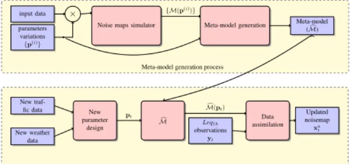
• Meta-modeling: quickly approximates the noisemap output of the model with a model. A meta-model is a way to estimate how a noisemap behaves
Noise maps simulator input data
parameters variations {p(i)}
×
Meta-model generation Meta-model ( cM) {M(p(i))}
Meta-model generation process New
traf-fic data New parameter
design New weather
data
c
M Leq1h assimilationData
observations yt pt Updated noisemap xa t c M(pt)
Figure 1. functional diagram of the data assimilation pro-cess, each significant block is described in the indicated paragraph
regarding some small variations of its parameters. Meta-models for noisemaps have been studied in a previous work [2]
• Data assimilation: Provides an analysis map which combines both the data from the simulation and the data from the observation.
A validation phase will be executed with a leave-one-out cross validation method.
2. DATA ASSIMILATION
The solution which will be used in this work is called BLUE, for Best Linear Unbiased Estimator. Starting with the output of the meta-model, a correction layer is super-posed, which depends on B, the covariance matrix of the error between the simulation at the observation points and the observed values, R, the covariance matrix of the obser-vation error and the real time estimation error.
At each timestep, a so-called background map xb = c
M(p) ∈ Rn is computed as shown in the functional
dia-gram in figure 1, it is an estimation of the real state noise level distribution field xt. It is impossible to know the
ex-act value xtwhether from the simulator or from the
sen-sors. In addition a set of observations y ∈ Rp is given. Let:
• H ∈ Rp×nbe the observation matrix which maps xt to the observed values y, so that y is the observation of the state Hxt.
• eb be the simulation error , eo be the observation error and B and R their respective covariance ma-trices.
Based on xb, B, y, R and H, an analysis state vector xa
is computed as the so-called “Best Linear Unbiased Esti-mator” which is linearly dependant on xband y, has unbi-ased error ea = xa− xt, and has a variance with minimum
trace. This estimator is uniquely defined as
xa= xb+ K(y − Hxb) (1) where
K = BHT(HBHT + R)−1 (2)
3. RESULTS: CROSS VALIDATION
An experiment has been conducted in an area of Paris, France of 3 km2with a grid of 8456 receivers and a net-work of 16 observation points on a time period of 9 months in 2015.
The leave-one-out cross-validation consists in removing the observations of a given microphone from the data as-similation process. Only the observations from the other microphones are used to correct the noise level distribu-tion. This procedure is carried out for all microphones, one by one, only one microphone is removed at a time. At the removed station, the meta-model performance is com-pared to the performance after assimilation of the obser-vations of the other microphones. This enables to check whether the assimilation properly distributes in space the corrections that originate from the observed locations. The cross-validation evaluates the effects of the data assimila-tion method at locaassimila-tions without any observaassimila-tions.
Figure 2 shows how the correction due to the observa-tions propagates across the study area. It follows the in-tuition that the more an observation point is overestimated (resp. underestimated) the more its neighborhood will have a negative correction (resp. positive).
250 0 250 500 750 1000 m error < -6 -6.0 - -4.0 -4.0 - -2.0 -2.0 - 0 0 0 - 2.0 2.0 - 4.0 4.0 - 6.0 > 6 xa < -6 -6.0 - -4.0 -4.0 - -2.0 -2.0 - 0 0 0 - 2.0 2.0 - 4.0 4.0 - 6.0 > 6
Figure 2. This map displays an example of the correction given by the observations at a given time.
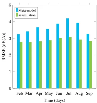
This reduction of the variance is noticeable in figure 3 where the root mean squared error is displayed at each
month for each step of the data assimilation process. At each step the RMSE is reduced and goes from an aver-age of 3.6 dB(A) with the annual simulation only (up to 4.2 dB(A) during the month of August) down to an aver-age of 2.9 dB(A) at the final staver-age.
Feb Mar Apr May Jun Jul Aug Sep 0 1 2 3 4 5 Time (days) RMSE (dB (A)) Meta-model assimilation
Figure 3. RMSE in dB(A) of the error between the obser-vation and the background (blue) or the analysis in leave-on-out cross-validation (green)
4. CONCLUSION
The data assimilation applied to noisemaps generated through a meta-model favorably improves the performance of the generated noisemap (from an average RMSE of 3.85 dB(A) to 2.78 dB(A)) and allows to grasp the hour to hour evolution of the noise level distribution across the study area.
5. ACKNOWLEDGMENTS
The authors would like to thank the CENSE project team for initiating this project, the Agence Nationale de la Recherche (ANR) for their financial support, the city of Paris and BRUITPARIF for granting access to their data and Nicolas Fortin of the UMRAE/IFSTTAR department for his technical support on the NoiseModelling software.
6. REFERENCES
[1] W. Wei, T. Van Renterghem, B. De Coensel, and D. Botteldooren, “Dynamic noise mapping: A map-based interpolation between noise measurements with high temporal resolution,” Applied Acoustics, vol. 101, pp. 127–140, 01 2016.
[2] A. Lesieur, P. Aumond, A. Can, and V. Mallet, “Meta-modeling for urban noise mapping,” in International Commission for acoustics, 2019.