Assimilation of GRACE data into the MESH model to improve the estimation of snow water equivalent

(1)

Département de Géomatique Appliquée

Faculté des Lettres et Sciences Humaines

Université de Sherbrooke

Assimilation des données GRACE dans le modèle MESH pour

l’amélioration de l'estimation de l'équivalent en eau de la neige

Assimilation of GRACE data into the MESH model to

improve the estimation of snow water equivalent

Ala Bahrami

Directeur de recherche: Kalifa Goïta Codirecteur de recherche: Ramata Magagi

Thèse présentée pour l'obtention du grade Philosophiae Doctor (PhD) en télédétection, cheminement en physique de la télédétection

August 2020 ©Ala Bahrami, 2020

(2)

(3)

Identification du jury

Directeur de recherche: Professor Dr. Kalifa Goïta, Université de Sherbrooke, Canada

Codirecteur de recherche: Professor Dr. Ramata Magagi, Université de Sherbrooke, Canada Membre du jury externe: Professor Dr. Barton Forman, University of Maryland, USA

Membre du jury interne: Professor Dr. Alexandre Langlois, Université de Sherbrooke, Canada Membre du jury interne: Professor Dr. Yacine Bouroubi, Université de Sherbrooke, Canada

(4)

Abstract

Water storage changes over space and time play a major rule in the Earth’s climate system through the exchange of water and energy fluxes among the Earth’s water storage compartments and between atmosphere, continents, and oceans. In many parts of northern-latitude areas spring meltwater controls the availability of freshwater resources. With respect to terrestrial hydrologic process, snow water equivalent (SWE) is the most critical snow characteristic to hydrologists and water resource managers. The first objective of this study examined the spatiotemporal variations of terrestrial water storages and their linkages with SWE variabilities over Canada. Terrestrial water storage anomaly (TWSA) from the Gravity Recovery and Climate Experiment (GRACE), the WaterGAP Global Hydrology Model (WGHM), and the Global Land Data Assimilation System (GLDAS) were employed. SWE anomaly (SWEA) products were provided by the Global Snow Monitoring for Climate Research version 2 (GlobSnow2), Advanced Microwave Scanning Radiometer‐Earth Observing System (AMSR-E), and Canadian Meteorological Centre (CMC). The grid cell (1°×1°) and basin-averaged analyses were applied to find any possible relationship between TWSA and SWEA over the Canadian territory, from December 2002 to March 2011. Results showed that GRACE versus CMC provided the highest percentage of significant positive correlation (62.4% of the 1128 grid cells), with an average significant positive correlation coefficient of 0.5, and a maximum of 0.9. In western Canada, GRACE correlated better with multiple SWE data sets than GLDAS. Yet, over eastern Canada, mainly in the northern Québec area (~ 55ºN), GRACE provided weak or insignificant correlations with all snow products, while GLDAS appeared to be significantly correlated. For the TWSA-SWEA analysis at the basin-averaged scale, significant relationships were observed between TWSA and SWEA for most of the fifteen basins considered (53% to 80% of the basins, depending on the SWE products considered). The best results were obtained with the CMC SWE products, compared to satellite-based SWE data. Stronger relationships were found in snow-dominated basins (Rs >= 0.7), such

as the Liard [root mean square error (RMSE) = 21.4 mm] and Peace Basins (RMSE = 26.76 mm). However, despite high snow accumulation in northern Québec, GRACE showed weak or insignificant correlations with SWEA, regardless of the data sources. The same behavior was observed in the western Hudson Bay Basin. In both regions, it was found that the contribution of non-SWE compartments, including wetland, surface water, as well as soil water storages has a

(5)

significant impact on the variations of total storage. These components were estimated using the WGHM simulations and then subtracted from GRACE observations. The GRACE-derived SWEA correlation results showed improved relationships with three SWEA products (CMC, GlobSnow2, AMSR-E). The improvement is particularly important in the sub-basins of the Hudson Bay, where very weak and insignificant results were previously found with GRACE TWSA data. GRACE-derived SWEA showed a significant relationship with CMC data in 93% of the basins (13% more than GRACE TWSA). In general, results revealed the importance of SWE changes in association with the terrestrial water storage (TWS) variations.

The second objective of this thesis investigates whether integration of remotely sensed terrestrial water storage (TWS) information, which is derived from GRACE, can improve SWE and streamflow simulations within a semi-distributed hydrology land surface model. A data assimilation (DA) framework was developed to combine TWS observations with the MESH (Modélisation Environnementale Communautaire – Surface Hydrology) model using an ensemble Kalman smoother (EnKS). This study examined the incorporation and development of the ensemble-based GRACE data assimilation framework into the MESH modeling framework for the first time. The snow-dominated Liard Basin was selected as a case study. The proposed assimilation methodology reduced bias of monthly SWE simulations at the basin scale by 17.5% and improved unbiased root-mean-square difference (ubRMSD) by 23%. At the grid scale, the DA method improved ubRMSD values and correlation coefficients of SWE estimates for 85% and 97% of the grid cells, respectively. Effects of GRACE DA on streamflow simulations were evaluated against observations from three river gauges, where it could effectively improve the simulation of high flows during snowmelt season from April to June. The influence of GRACE DA on the total flow volume and low flows was found to be variable. In general, the use of GRACE observations in the assimilation framework not only improved the simulation of SWE, but also effectively influenced the simulation of streamflow estimates.

Key words: Gravity Recovery and Climate Experiment (GRACE), Terrestrial Water Storage

(TWS), MESH (Modélisation Environnmentale Communautaire – Surface Hydrology), Snow Water Equivalent (SWE), Data Assimilation (DA), Ensemble Kalman smoother (EnKS).

(6)

Résumé

Les variations dans l'espace et le temps du stock d'eau à travers jouent un rôle important dans le système climatique de la Terre à travers l'échange des flux d'eau et d'énergie entre les compartiments du stock d’eau de la Terre, et entre l'atmosphère, les continents et les océans. Dans les régions nordiques, la fonte de la neige contrôle la disponibilité des ressources en eau. Concernant le processus hydrologique terrestre, l'équivalent en eau de la neige (SWE) est la caractéristique de neige la plus importante pour les hydrologues et les gestionnaires des ressources en eau. Le premier objectif de cette étude a examiné les variations spatio-temporelles des réservoirs terrestres d'eau et leurs liens avec les variabilités de SWE au Canada. Des anomalies de stockage d'eau terrestre (TWSA) provenant de GRACE (Gravity Recovery and Climate Experiment), du modèle hydrologique mondial WaterGAP (WGHM) et du modèle GLDAS (Global Land Data Assimilation System) ont été utilisées. Les produits du SWEA (Snow Water Equiavalent Anomaly) sont fournis par le GlobSnow2 (Global Snow Monitoring for Climate Research version 2), le AMSR-E (Advanced Microwave Scanning Radiometer‐Earth Observing System) et le Centre météorologique canadien (CMC). L'analyse par cellule de grille (1°×1°) a été appliquée pour trouver toute relation possible entre TWSA et SWEA sur le territoire canadien, de décembre 2002 à mars 2011. Les résultats montrent que GRACE par rapport à CMC a fourni le pourcentage le plus élevé de corrélation positive significative (62,4% des 1128 cellules de la grille), avec un coefficient de corrélation positif significatif moyen de 0,5 et un maximum de 0,9. Dans la partie ouest du pays, GRACE a montré un meilleur accord avec plusieurs produits SWE que GLDAS. Pourtant, dans l'est du Canada, principalement dans le nord du Québec (~ 55° N), GRACE a fourni des corrélations faibles ou insignifiantes avec tous les produits SWE, contrairement à GLDAS qui semblait être significativement corrélé. Dans le cas de l’analyse à l'échelle du bassin versant, les relations significatives ont été observées entre TWSA et SWEA pour la plupart des quinze bassins considérés (53% à 80% des bassins, selon les produits SWE considérés). Les meilleurs résultats ont été obtenus avec les produits CMC SWE, par rapport aux données SWE satellitaires. Des relations plus fortes ont été trouvées dans les bassins dominés par la neige (Rs> = 0,7), tels que le bassin versant de Liard [erreur quadratique moyenne (RMSE) = 21,4 mm] et le bassin versant de Peace (RMSE = 26,76 mm). Cependant, malgré une forte accumulation de neige dans le nord du Québec, GRACE a montré des corrélations faibles ou insignifiantes avec SWEA, peu importent

(7)

les sources de données. Le même comportement a été observé dans le bassin versant ouest de la Baie d’Hudson. Dans les deux régions, il a été constaté que la contribution des compartiments non-SWE, y compris les zones humides, les eaux de surface, ainsi que les stocks d'eau du sol a un effet significatif sur les variations du stock total. Ces composantes ont été estimées à l'aide des simulations du modèle WGHM, puis soustraites des observations GRACE. Ces résultats de corrélation SWEA dérivés de GRACE ont montré une amélioration des relations avec les trois produits SWE (CMC, GlobSnow2, AMSR-E). L'amélioration est particulièrement importante dans les sous-bassins de la Baie d’Hudson, où des résultats très faibles et insignifiants avaient été précédemment trouvés avec les données GRACE TWSA. La SWEA dérivée de GRACE a montré une relation significative avec les données CMC dans 93% des bassins (13% de plus que GRACE TWSA). En somme, les résultats obtenus dans ce premier objectif ont montré le rôle important du SWE dans les variations du stock terrestre de l'eau dans la région d’étude.

Le deuxième objectif de cette thèse examine si l'intégration des informations de TWS (terrestrial water storage) dérivées de GRACE (Gravity Recovery and Climate Experiment), peut améliorer les simulations du SWE et du débit d’eau dans un modèle hydrologique semi-distribué de schéma de surface. Un cadre d'assimilation de données (DA) a été développé pour combiner les observations TWS avec le modèle MESH (Modélisation Environnementale Communautaire - Hydrologie de Surface) en utilisant un ensemble Kalman Smoother (EnKS). Cette étude était la première du genre à tenter une assimilation des données GRACE dans le modèle MESH pour améliorer l’estimation du SWE. Le bassin versant de la Liard dominé par la neige a été choisi pour le site d’étude. À l’échelle du bassin versant, la méthodologie d'assimilation proposée a réduit le biais des simulations mensuelles de SWE à 17,5% et amélioré le ubRMSD (unbiased root-mean-square difference) de 23%. À l'échelle de la grille, la méthode DA a amélioré l’estimation du SWE pour les valeurs ubRMSD et les coefficients de corrélation pour 85% et 97% des cellules de la grille, respectivement. Les effets de GRACE DA sur les simulations de débit ont été évalués par rapport aux observations de trois stations des débits, où il pourrait effectivement améliorer la simulation des débits élevés pendant la saison de fonte de la neige d'avril à juin. L'influence de GRACE DA sur le volume total et les faibles débits d’eau a été trouvée variable. En général, l'utilisation des observations GRACE dans le cadre d'assimilation non seulement a amélioré la simulation de SWE, mais a également influencé efficacement la simulation des estimations de débit.

(8)

Mots-clés: Gravity Recovery and Climate Experiment (GRACE), Stock d'eau Terrestre (TWS),

MESH (Modélisation Environnmentale Communautaire – Surface et Hydrologie), équivalent en eau de la neige (SWE), Assimilation de Données (DA), Ensemble Kalman smoother (EnKS).

(9)

List of Figures

Figure 1.1. The schematic overview of the Earth’s water movement ... 2

Figure 1.2. The evaluation of modeled and observed SWE over 12 year period. Left images present the time mean of SWE (mm) in March for CLASS, CMC, and GlobSnow. Left images show seasonal cycles of the total modeled, land only (exclusion of lakes), CMC, and GlobSnow SWE for the tundra, boreal, and southern zones. ... 7

Figure 2.1. GRACE mission concept. ... 14

Figure 2.2. GRACE and GRACE-FO mission data flow. ... 16

Figure 2.3. Mackenzie GEWEX Study (MAGS) modeling strategy. ... 20

Figure 2.4. MESH modeling framework. ... 22

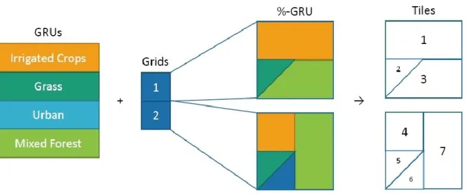
Figure 2.5. The GRU approach to basin discretization used in MESH ... 24

Figure 2.6. Schematic diagram of CLASS ... 25

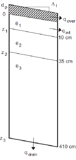
Figure 2.7. Soil moisture and land-surface drainage representation in MESH-CLASS. In this figure dp, z, θ, Λ, and q present water ponded on the surface, soil depth, volumetric soil moisture, soil slope, and flow respectively. ... 27

Figure 2.8. Runoff routing concept ... 28

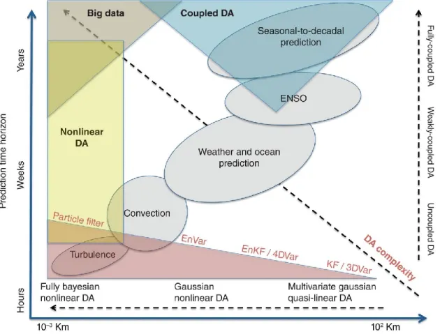
Figure 2.9. Required data assimilation method based on mode resolution and prediction time horizon ... 30

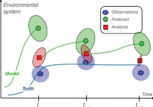
Figure 2.10. Illustration of sequential data assimilation. Observations (blue), forecast (green), and analysis (red). The true signal is presented by the blue line, ... 31

Figure 3.1. Map of land cover types. ... 42

Figure 3.2. Map of digital elevation model (DEM ). ... 43

Figure 3.3. Location of the fifteen Canadian river basins ... 43

Figure 3.4. Mackenzie and Liard basin boundary discretizations. ... 45

Figure 3.5. General methodology of this study ... 53

(16)

Figure 4.2. Flowchart for analyzing the TWSA-SWEA relationship. ... 64 Figure 4.3. Gridded correlation coefficient analysis between GRACE/GLDAS-derived TWSA

and GlobSnow2/AMSR-E/CMC-derived SWEA: (a) results for GRACE and GlobSnow2; (b) results for GLDAS and GlobSnow2: (c) results for GRACE and AMSR-E: (d) results for GLDAS and AMSR-E: (e) results for GRACE and CMC: (f) results for GLDAS and CMC... 67

Figure 4.4. Gridded p-value analysis between GRACE/GLDAS-derived TWSA and

GlobSnow2/AMSR-E/CMC-derived SWEA: (a) results for GRACE and GlobSnow2; (b) results for GLDAS and GlobSnow2: (c) results for GRACE and AMSR-E: (d) results for GLDAS and AMSR-E: (e) results for GRACE and CMC: (f) results for GLDAS and CMC. ... 68

Figure 5.1. Overview location of the fifteen Canadian river basins considered. Information about

the basin is presented in Table 5.1. ... 90

Figure 5.2. Flowchart for preprocessing and comparing GRACE-derived TWSA/SWEA to the

multisource SWEA products. ... 92

Figure 5.3. WGHM time mean storage compartment, including canopy, wetland, groundwater,

surface water, SWE, and soil moisture in the fifteen studied basins during the snow seasons from 2002 to 2011. ... 95

Figure 5.4. Basin-average DJFM time series of GRACE TWSA, CMC SWEA, GlobSnow2

SWEA, AMSR-E SWEA, and GRACE SWEA for the Fraser, Churchill, Southwestern of Hudson Bay, La Grande, Nelson, Northeastern Hudson Bay, Nottaway, Ungava Bay Basins from December 2002 until March 2011. ... 96

Figure 5.5. Basin-average DJFM time series of GRACE TWSA, CMC SWEA, GlobSnow2

SWEA, AMSR-E SWEA, and GRACE SWEA for the Western Hudson Bay, Athabasca, Bear and Peel, Liard, Peace, Slave, Saint Lawrence River Basins from December 2002 until March 2011... 97

Figure 6.1. Map of the Liard Basin, including the digital elevation model (DEM), basin

boundary, locations of streamflow observations, and automated snow survey locations (triangles). Red circles indicate three river stations: (A) Liard River Near the Mouth ; (B) Liard River at Fort Liard; and (C) Liard River at Lower Crossing. ... 124

(17)

Figure 6.3. Time Series of MESH-derived TWS estimates from the OL (dark gray), DA (light

gray) simulation, and the GRACE observations with the error bar of 17 mm in the Liard Basin. The dark and light gray areas show the ranges of OL and DA ensembles, while the thick dashed and solid lines correspond to the respective ensemble means. ... 134

Figure 6.4. Time Series of MESH-derived SWE estimates in the Liard Basin on the left Y-axis

and their corresponding ensemble spreads on the right Y-axis. OL and DA ensemble means are shown with solid black and brown lines, respectively. Monthly CMC SWE estimates are represented with solid red circles. OL and DA ensemble spreads are respectively indicated by black and brown dashed lines. ... 135

Figure 6.5. Evaluation of the open-loop (OL) and the data assimilation (DA) approaches using

Percent bias (PBIAS), unbiased root-mean-square difference (ubRMSD), and Spearman’s rank correlations (Rs). ... 136 Figure 6.6. Evaluation results of the ubRMSD [mm] of SWE from the OL (A) and the skill

difference [mm] between GRACE DA and OL methods (B). Black dots indicate grid cells where the ubRMSD differences are statistically significant at the 95% confidence intervals. ... 138

Figure 6.7. Evaluation results of Spearman’s rank correlations (Rs) of SWE from the OL (A) and

the skill difference ΔRs between GRACE DA and OL methods (B). Black dots indicate grid cells

where the correlation differences between DA and OL results are statistically significant according to their respective 95% confidence intervals. ... 140

Figure 6.8. Time mean ensemble spread at gridded scale from October 2008 to October 2014 for

OL (A) and the difference between ensemble spread of the GRACE DA and OL (B). ... 141

Figure 6.9. Monthly time series comparison of SWE estimates from the OL (black), DA (gray),

snow survey observations (blue), and CMC (red) at three snow survey stations: (A) 4C22P, (B)4C21P, and (C) 4C20P. ... 143

Figure 6.10. Time series of the river streamflow estimates on the left Y-axes and their

corresponding ensemble spreads on the right Y-axes at three river stations: (A) Liard River Near the Mouth, (B) Liard river at Fort Liard; and (C) Liard River at Lower Crossing. Solid black and brown lines represent the OL and DA ensemble averages, respectively. Observed streamflows are shown with green solid lines. The OL and DA ensemble spreads are shown as black and brown dashed lines, respectively. ... 146

(18)

Figure 6.11. Normalized Innovation (NI) statistics for the Liard Basin. The different marker

colors correspond to four data assimilation experiments based on observation error variance of 72.25 mm2_{(red circle), 289 mm}2_{(blue square), 650.25 mm}2_{(green diamond), and 1156 mm}2

(purple star). ... 153

Figure 6.12. Time series of analysis increments for the Liard Basin from October 2008 to October

2014. The solid blue and black lines show monthly mean analysis increments that were calculated for SWE and the subsurface, respectively. ... 155

(19)

List of Tables

Table 1.1. Estimates of storage in primary global hydrologic reservoirs ... 1

Table 2.1. Summary of GRACE data assimilation experiments into the CLSM and CLM models ... 38

Table 2.2. Summary of GRACE data assimilation experiments into the WGHM and W3RA models ... 39

Table 2.3. Summary of GRACE data assimilation experiments into the HBV-96 and PCR-GLOBWB models ... 40

Table 3.1. Basin areas, forest fractional cover, and elevation. Basin locations can be seen in Figure 3.3. ... 44

Table 3.2. Pros and Cons of datasets ... 49

Table 3.3. Pros and Cons of datasets ... 50

Table 4.1. Summary of the SWE data sets used in this study. ... 63

Table 4.2. Summary of gridded correlation statistics of the comparison between GRACE/GLDAS-derived TWSA and SWEA from GlobSnow2, AMSR-E, and CMC. ... 69

Table 5.1. Basin areas, forest fractional cover, and elevation. Location of the basins can be seen in Figure 5.1. ... 90

Table 5.2. Basin averaged statistical results between GRACE derived TWSA and SWEA and GlobSnow2/AMSR-E/CMC SWEA for fifteen basins from December 2002 to March 2011. Entries marked with an asterisk indicate insignificant Rs results... 98

Table 5.3. Basin averaged RMSE results between GRACE derived TWSA and SWEA and GlobSnow2/AMSR-E/CMC SWEA for fifteen basins from December 2002 to March 2011. .... 98

Table 6.1. Perturbation parameters for model state and meteorological forcing ... 130

Table 6.2. Summary of PBIAS, ubRMSD, and Rs skills for OL and GRACE DA at three snow survey stations. Results obtained with CMC for the grid cell corresponding to each station location are also shown. ... 144

(20)

Table 6.3. Summary of PBIAS, NSE, and NSElog skills for OL and GRACE DA at three river

(21)

Acronyms

AI Analysis Increments

AMSR-E Advanced Microwave Scanning Radiometer for Earth Observing System

ANU Australian National University

CaPA Canadian Precipitation Analysis

CCMEO Canada Centre for Mapping and Earth Observation

CCRS Canada Centre for Remote Sensing

C/DA Calibration and Data Assimilation

CDED Canadian Digital Elevation Data

CMC Canadian Meteorological Centre

CLASS Canadian Land Surface Scheme

CaLDAS Canadian Land Data Assimilation System

CLM Community Land Model

CRCM Canadian Regional Climate Model

CSR Center for Space Research

DA Data Assimilation

DCS Data Collection System

DEM Digital Elevation Model

DLR Deutsches Zentrum für Luft- und Raumfahrt

DZTR Dynamically Zoned Target Release

EAKF Ensemble Adjustment Kalman Filter

ECCC Environment and Climate Change Canada

EnKF Ensemble Kalman filter

EnKS Ensemble Kalman Smoother

EnSRF Ensemble Square-Root Filter

FFT Fast Fourier Transform

(22)

GEM Global Environmental Multiscale

GEM-Hydro GEM Hydrological

GFZ GeoforschungsZentrum Potsdam

GIA Glacial Isostatic Adjustment

GIWS Global Institute for Water Security

GlobSnow Global Snow Monitoring for Climate Research

GLDAS Global Land Data Assimilation System

GMAO Global Modeling and Assimilation Office

GOES Geostationary Satellites

GPS Global Positioning System

GRACE Gravity Recovery and Climate Experiment

GRACE-FO GRACE Follow-On

GRU Grouped Response Units

H-LSM Hydrological and Land Surface Models

JPL Jet Propulsion Laboratory

LAI Leaf Area Index

LCC Land Cover of Canada

LQWS Liquid Water Storage

LRI Laser Ranging Interferometer

LSM Land Surface Model

LZS Lower Zone Storage

MAGS Mackenzie GEWEX Study

MCMC Markov Chain Monte Carlo

MEC Modélisation Environnementale Communautaire

MESH Modélisation Environnementale Communautaire – Surface Hydrology

MESH-CLASS MESH and CLASS

MESH-GRACE MESH and GRACE

MODIS Moderate Resolution Imaging Spectroradiometer

(23)

NASA National Aeronautics and Space Administration NOAA National Oceanic and Atmospheric Administration

NSE Nash-Sutcliffe Efficiency

NSIDC National Snow and Ice Data Center

NWP Numerical Weather Prediction

OL Open-Loop

PBIAS Percentage Bias

PBSM Prairie Blowing Snow Model

PCR-GLOBWB PCRaster Global Water Balance

PDF Probability Density Functions

PDMROF Probability Distribution Model based RunOff

PF Particle Filters

PFT Plant Functional Type

PMW Passive Microwave

R&D Research and Development

RMSD Root Mean Square Difference

RMSE Root Mean Square Error

SD Snow Depth

SDS Science Data System

SEIK Singular Evolutive Interpolated Kalman

SLC Soil Landscapes of Canada

SMOS Soil Moisture and Ocean Salinity

SnowMIP Snow Model Intercomparison Project

SQRA Square Root Analysis

SVS Soil, Vegetation, and Snow

SWE Snow Water Equivalent

SWEA Snow Water equivalent Anomaly

(24)

TWS Terrestrial Water Storage

TWSA Terrestrial Water Storage Anomaly

UbRMSD Unbiased Root-Mean-Square Difference

WaterGAP Water-Global Assessment and Prognosis

WGHM WaterGAP Global Hydrology Model

WSC Water Survey of Canada

W3RA World-Wide Water Resources Assessment

(25)

Acknowledgments

First of all, I would like to thank my supervisor Prof. Dr. Kalifa Goïta who offered me this opportunity to undertake my PhD studies at Université de Sherbrooke. I am very grateful for all the supports, valuable suggestions, guidance and freedom that gave me the opportunity to build my own research profile. His valuable insights and professional attitudes helped me to improve the results of this work through the process from beginning to end. Extended gratitude also goes to my co-supervisor Prof. Dr. Ramata Magagi for her generous support of my work, her patience and inspiration, and her immense knowledge in helping me to manage the complex task of completing this work. I would like to acknowledge the financial supports, awarded by the Natural Sciences and Engineering Research Council of Canada (NSERC).

My deep gratitude goes to Prof. Dr. Barton Forman (University of Maryland, USA), Prof. Dr. Alexandre Langlois (Université de Sherbrooke, Canada), and Prof. Dr. Yacine Bouroubi (Université de Sherbrooke, Canada) for their evaluations of my thesis. Their constructive comments helped me to improve the quality of this dissertation.

During my PhD studies, I had the unique chance to spend six months as a visiting researcher in the School of Environment and Sustainability at the University of Saskatchewan. I would like to thank the researchers and employees of the Environment and Climate Change Canada, Global Institute for Water Security, and the Centre for Hydrology at the University of Saskatchewan. I would like to acknowledge and thank Dr. Bruce Davison for providing me this chance to collaborate with a group of researchers in this project. His valuable guidance helped me to improve my skills and understanding through my PhD studies. My special thanks go to Prof. Dr. Saman Razavi for supporting me during my stay at Saskatoon to work in a productive and friendly environment. Very special thanks go to Dan Princz who has provided me valuable insights and suggestions that without doubts helped me to deal with technical programming issues of MESH open-source software. I would thank Mohamed Elshamy for taking his time and providing technical and scientific supports regarding the MESH configuration, and analysis of the model outputs. His helpful suggestions had a tremendous positive impact on my experience. I would like to thank Dr. Amin Haghnegahdar for the fruitful discussions during my stay in Saskatoon. I am grateful for the administrative support of Michelle Martel-Andre who helped me with her warm

(26)

and friendly guidance during my visit to Saskatoon.

During my PhD studies, I had the unique chance to have fruitful discussions with Dr. Ally M. Toure, Dr. Alexandre Roy, Dr. Hannes Müller Schmied, and Dr. Ehsan Forootan. I would also like to thank the faculty and staff at Université de Sherbrooke for all their work and support through different stages of my studies. I like to thank Odile Couture who helped me with her smiles to cope with administrative tasks. I would like to thank my colleagues at Université de Sherbrooke. During my graduate studies, I met many nice, friendly, outgoing colleagues who inspired me a lot for having various social and sportive activities. My special thanks go to Jean-Benoît Madore (JB) for his tremendous support and help. I like to thank: Brice Caillié, Nicolas Marchand, Bruno-Charles Busseau (BC), Joris Ravaglia, Michael Prince, Olivier Saint-Jean-Rondeau, Daniel Kramer, Simon Levasseur, Guillaume Couture, Julien Meloche, Ali Ben Abbes, Florentin Bourge, Paul Billecocq, Carina Poulin, Homayoun Harirforoush, Joëlle Voglimacci, Vincent Beauregard, Nathalie Thériault, Caroline Dolant, Fanny Larue, Adrien Letellier, Vincent Sasseville, Céline Vargel, and Alex Mavrovic.

I am fortunate in my life to have a group of adorable friends. I am very grateful to my best friend Arvin Morattab. I always enjoyed spending time with him. The loss of Arvin and his lovely wife Aida, in the crash of Ukrainian flight PS752, was an unbelievable tragedy for me. I owe particular thanks to Armin Morattab, Arash Morattab, Fereshteh Farokhi, Saman Pournahavandi, Iraj Yadegari, Hamid Dehghan, Jamil Bahrami, Babak Hejrani, Fardin Nili, and Babak Roshani. I would like to thank my parents, Sheida and Alaeddin, who have stood beside and supported me in entire life. Special thanks also go to my lovely and supportive sister and brother, Nishtman and Azad, who have always encouraged and inspired me with their kind motivations and inspirations throughout my life. Without the support of my family, none of this work would have been possible, and their contribution is unmatched by my own effort. I would like to thank my uncle, Saadi, for his encouragement and kind assistance during my life.

Finally, but very certainly not least, my most warm and exceptional gratitude goes to Soma for bearing me during this adventure, particularly during difficult times. She has filled my life with so much joy and supported me in all aspects. Finishing this thesis would not be possible without her immense support.

(27)

Reading Guide

As part of this research project, we have published one article in the Hydrological Processes Journal. One article has been also submitted to the Journal of Hydrology. One article is also prepared for submission to the Journal of Remote Sensing.

Therefore, this thesis is presented in the form of articles based on three journal publication/submissions. Three technical chapters of the thesis are devoted to the articles. Each chapter contains the following sections: introduction, study site and data, methodology, results, and discussion. Chapter 1 explains the research problematics, objectives, research questions, and hypotheses. Chapter 2 is an overview of the scientific background and applications. Chapter 3 explains the summary of datasets and study sites. Chapters 4, 5, and 6 in the form of articles, present the TWSA-SWEA relationship analysis and data assimilation implementation, respectively. Chapter 7 is dedicated to overall discussions. Finally, the findings of the thesis, general perspectives, and outlooks are described in chapter 8.

(28)

1. Introduction

1.1. The Global water cycle

Continental water storage changes in space and time play a major rule in the Earth’s climate system via the exchange of water and energy fluxes among the Earth’s water storage compartments and between atmosphere, continents, and oceans (Döll et al., 2014a). Global observations of water and ice mass distribution at monthly to decadal time scales are crucial for the forecast of climate change, weather, biological and agricultural productivity, flooding, and a wide variety of studies in the geoscience (Rodell et al., 2004; Tapley et al., 2019). Thus, the critical challenge for this century may be the globally sustainable management of water resources (Rodell et al., 2018).

Terrestrial water storage (TWS) as a major variable of the Earth’s water cycle is defined as the summation of key hydrologic reservoirs, including soil water (i.e, near surface in unsaturated zone and in deeper groundwater reservoirs), surface water (i.e., rivers, lakes), the cryosphere water storage (including seasonal snowpack, mountain glaciers, polar ice sheets), and biomass water storage (Famiglietti and Rodell, 2013; Margulis, 2014). In Table 1.1 the approximate estimate of water storage in the key reservoirs in the global system is presented. After the ocean reservoir, the largest source of water storage is the ice caps and glaciers which contain valuable sources of freshwater in frozen form (Margulis, 2014).

Table 1.1. Estimates of storage in primary global hydrologic reservoirs (Bras, 1990)

Reservoir Volume (km3₎ _{% Total water}

Oceans 1,322,000,000 97.2

Ice caps & glaciers 29,199,700 2.1

Groundwater (near surface) 4,171,400 0.31

Lakes & rivers 130,700 0.017

Soil moisture 66,700 0.005

(29)

The general schematic of water distribution in surface and sub-surface water storage, as well as mass variation within and between ocean and atmosphere, is presented in Figure 1.1.

Figure 1.1. The schematic overview of the Earth’s water movement (Retrieved from https://www.usgs.gov/media/images/water-cycle-natural-water-cycle)

1.2. The importance of snow

Snow as one of the most noticeable elements of the hydrologic cycle has considerable influence on the short- and long-term weather and climate systems of various regional and hemispheric phenomena (Cohen and Entekhabi, 1999; Su et al., 2010; Walsh, 1984). In the Northern hemisphere, energy budget, water balance, and geochemical cycles are influenced by the seasonal cycle of the terrestrial snow and snow mass (Mudryk et al., 2015). Snow is a critical component of the hydrologic cycle due to the pivotal impact of snow albedo (reflectivity) and surface temperature feedbacks on weather and climate (Barnett et al., 1989; Cohen, 1989; Fletcher et al., 2009; Gong et al., 2004; Kelly, 2009; Robinson et al., 1993; Yang et al., 2001). There are different

(30)

ways in which snow cover alters the exchange of energy between the surface and the atmosphere. First, the albedo of fresh snow is 0.8-0.85 for sunlight, while the reflectivity of bare land and ice-free ocean is typically between 0.05 and 0.3 (Walsh, 1984). Therefore, snowpack helps to cool the surface temperature due to high albedo of snow, more outgoing thermal radiation due to high emissivity of snow, and more outgoing heat flux due to snowmelt, evaporation and/or sublimation (Gong et al., 2004). Second, snow as a highly effective insulator has low thermal conductivity. The soil temperature can remain unfrozen for several weeks beneath a snow cover of 20-30 cm, even when the air temperature drops to 10-20º C below freezing point (Walsh, 1984).

In many parts of northern-latitude areas, as well as the mountainous regions, spring meltwater controls the availability of freshwater resources for approximately more than one-sixth of the world’s population (Barnett et al., 2005; Déry et al., 2005; Stieglitz et al., 2001). With respect to the terrestrial hydrologic process, three fundamental parameters for climatology and hydrology include snow water equivalent (SWE), snow extent, and melt onset (Foster et al., 2011). SWE is defined as the equivalent amount of liquid water mass that be acquired if the entire snowpacks were melted (Margulis, 2014). Thus, the accurate presentation of SWE is the most critical snow characteristic to hydrologists and water resource managers for operational run-off and river discharge forecasts (McCreight et al., 2014; Pulliainen, 2006). However, estimation of SWE over time and space is a challenging task.

1.3. SWE estimation

SWE can be estimated using ground-based techniques, remote sensing, and land surface model (LSM) simulations. Ground-based SWE information can be estimated using the interpolation of SWE in-situ measurements or as the product of snow depth (SD) and snow density observations. SD is easier and quicker to measure than SWE (Sturm et al., 2010). However, the accuracy of the snow depth measurements is influenced by the interpolation of observations from gauging networks and snow courses, or daily synoptic weather station-based measurements (Pulliainen, 2006). In addition to the limitations of snow depth products, snow density measurements (e.g., snow tubes, triangular sampler) have their uncertainties. Snow density has around 10% uncertainty in the density measurement. The uncertainty of SWE estimates is negatively influenced by inadequate spatial coverage, especially in the northern regions where observations become sparse

(31)

and also biased toward coastal location that may not be representative of the general area (Derksen et al., 2010; Rott et al., 2010; Verseghy et al., 2017b). Due to limitations of ground-based SWE methods, satellite remote sensing measurements and land surface model simulations are considered as alternative solutions to obtain more accurate snow products (Zhang et al., 2014). Among remote sensing SWE estimation approaches, satellite passive microwave (PMW) retrievals have been used since 1978 and SWE estimates have been offered at all weather conditions with good temporal (daily) and moderate (~25 km) spatial resolution. Despite the benefits of PMW SWE products, they have several major drawbacks in forest land cover types and wet and deep snow conditions (when SWE is higher than 150 mm). These limitations can cause high uncertainties (up to 50% in boreal forest) in SWE estimates such that the usage of PMW SWE retrievals faces important challenges (Chang et al., 1996; Roy, 2014; Roy et al., 2010, 2012; Vachon et al., 2010). Therefore, due to the limitations of PMW SWE estimates, other satellite remote sensing observations should be considered as alternative products. More information on SWE estimation using microwave remote sensing can be found in the work of Tedesco et al. (2014) and Saberi et al. (2020).

Among satellite measurement techniques, the Gravity Recovery and Climate Experiment (GRACE, Tapley et al., 2004a) added a unique component to the existing suite of Earth observations by measuring the redistribution of terrestrial water storage anomaly (TWSA) around the world. Water mass movement can influence the Earth’s gravity in a way that can be observed and quantified by gravity-based measurements (Reager, 2012). GRACE is a unique data source that can detect the spatiotemporal changes of the Earth’s water storage and improve the estimation of the water cycle at regional to global scales (Güntner, 2008). GRACE observations are fundamental to understand the complex interactions and transitions involved in today's changing climate (Tapley et al., 2019). The satellite observation of TWSA provides large-scale changes of total quantity of water as the summation of groundwater, soil moisture, SWE, surface water, ice, and water in biomass (Famiglietti and Rodell, 2013). This remote sensing product offers broad spatial coverage and provides much greater insight into global problems. The TWSA retrievals have monthly temporal resolution with an effective spatial (horizontal) resolution no better than a few hundred kilometers (Landerer and Swenson, 2012). GRACE unlike other satellite-based instruments, such as passive microwave sensors, does not rely on surface conditions and can measure total precipitation accumulation with no need for empirical parametrization and

(32)

ground-based calibration (Behrangi et al., 2017, 2018). Over snow-dominated areas, the total water storage changes captured by GRACE are highly dominated by snow mass changes during snow accumulation and ablation phase (Forman et al., 2012). In the mountainous regions during cold seasons, GRACE has provided the accumulated precipitation which appeared to be advantageous compared to conventional hydro-meteorological observing systems which faced the highest detection and retrieval uncertainty (Behrangi et al., 2017, 2018).

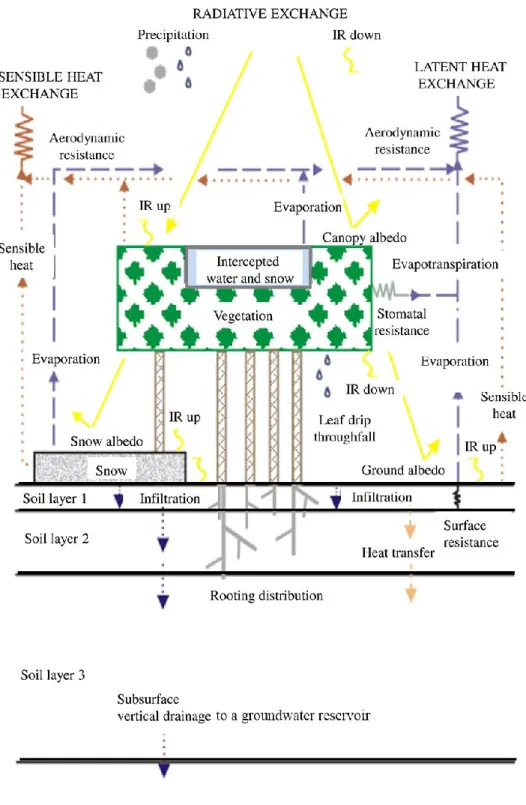
A large number of LSMs has been developed to simulate the spatiotemporal variability of TWS changes on small to large scales in order to improve the estimation of the global water cycle (Schumacher, 2016; Sood and Smakhtin, 2015). Environment and Climate Change Canada (ECCC) designed a community-based hydrological-land surface model (H-LSM) called MESH (Modélisation Environnementale Communautaire (MEC) – Surface Hydrology; Pietroniro et al., 2007). MESH, as a semi-distributed coupled model, has been developed for large-scale watershed modeling with consideration of cold region processes common in Canada. MESH is configured with the Canadian Land Surface Scheme (CLASS, Verseghy, 1991; Verseghy et al., 1993), the hydrological routing from WATFLOOD (Kouwen, 1988; Kouwen et al., 1993), and other lateral flow processes (Mekonnen et al., 2014; Soulis et al., 2000, 2011; Yassin et al., 2019). In this study, CLASS version 3.6 (Verseghy, 2012) is used to simulate the vertical energy and water fluxes for the vegetation canopy, snow, and different soil layers. The MESH model prognostic state (e.g., SWE) and flux simulation similar to other hydrological models are subject to several sources of uncertainty. Several important sources that influence model simulation include input data (e.g., climate forcing), model structure, and model parametrization (Müller Schmied et al., 2014). Therefore, it may be useful to constrain model-derived water storage states by using auxiliary information in order to improve model simulation (Schumacher, 2016).

1.4. Challenge of SWE estimation methods 1.4.1. Modeled SWE

The seasonal snowpack estimates in CLASS is simulated using a single thermal layer with a bulk temperature and surface skin temperature. The evaluation of CLASS-derived SWE estimates in the Snow Model Intercomparison Project (SnowMIP) demonstrated that the single-layer model performed well compared to the multi-layer snowpack (Brown et al., 2006; Essery et al., 2009;

(33)

Etchevers et al., 2002, 2004; Rutter et al., 2009).

The first performance of the MESH model configured with CLASS (MESH-CLASS) version 3.0 in the simulation of snow mass was evaluated in the Ottawa river basin (Pietroniro et al., 2007). The validation of results against snow survey observations showed that MESH-CLASS underestimated the SWE estimates. The Root Mean Square Error (RMSE) values of modeled SWE for years 2002 to 2005 fell between the range of 54 mm to 86 mm. The evaluation of MESH-CLASS in the SWE estimation has not been conducted in other studies. However, the individual performance of CLASS coupled with regional models was evaluated in a number of studies. Langlois et al. (2014) evaluated the modeled SWE of CLASS versions 2.7 and 3.5 coupled to the Canadian Regional Climate Model, version 4 (CRCM4) over northern Québec. The assessment of results against snow course data revealed an overall overestimation of SWE with the RMSE values of 78.8 mm and 73.9 mm for both experiments respectively. The results show that the uncertainty of the model in the estimation of SWE is quite higher than the expected uncertainty limits of 30 mm for SWE < 300 mm (Rott et al., 2010; Roy, 2014).

Recently, two studies evaluated the performance of CLASS-derived SWE estimates coupled to the CRCM5 on a regional scale over eastern and western Canada (Verseghy et al., 2017; Verseghy and MacKay, 2017). The assessment analysis for the 12-year period of 1998-2010 demonstrated that CLASS has a substantial positive bias compared to the Canadian Meteorological Center (CMC) SWE data for March to May in Labrador and in the northern part of the Quebec (Verseghy et al., 2017). Furthermore, for the first time over the western regions of Canada, the performance of CLASS was evaluated against monthly CMC and Global Snow Monitoring for Climate Research (GlobSnow) data sets, by excluding the mountainous regions (Verseghy and MacKay, 2017). The seasonal cycle of monthly modeled SWE (with and without lakes simulation), in addition to CMC and GlobSnow for the tundra, boreal, and southern zones are shown in Figure 1.2. Even though Verseghy and MacKay (2017) indicated that the CLASS model was deemed to have acceptable performance, they have not presented any statistical skill to illustrate the uncertainty of model simulation.

Based on the above-mentioned studies, valuable insights about the uncertainties and challenges in simulating snow mass using CLASS were highlighted. There is a substantial need to accurately

(34)

represent the snow budget. To achieve this objective, a robust method should be implemented to improve the modeled SWE estimation. Note that, the simulation of energy and water budgets within a tile (basin computational unit) in the MESH model is derived using different physically-based solver routines of the CLASS model. Then in the MESH model, the water storage, energy, and soil prognostic variables for each grid cell are weighted according to the land cover percentage area that is occupied inside the grid.

Figure 1.2. The evaluation of modeled and observed SWE over 12 year period. Left images present the time mean of SWE (mm) in March for CLASS, CMC, and GlobSnow. Left images show seasonal cycles of the total modeled, land only (exclusion of lakes), CMC, and GlobSnow SWE for the tundra, boreal, and southern zones (Verseghy and MacKay, 2017).

(35)

1.4.2. Estimation of SWE using GRACE observations

For the first time in the history of geoscience, satellite-based observations of global water cycle from the GRACE mission have provided the free-access of freshwater resource changes across the globe (Rodell et al., 2018). This unique potential of gravimetric measurements enables the analysis of TWS anomalies over the continents, river basin and local scales, which is not feasible using traditional microwave, infrared, or visible remote sensing measurements (Forman and Reichle, 2013). Even though GRACE observations are employed for different hydrological applications, different challenges are associated with TWS data.

Two main issues are linked to GRACE-derived TWSA products. First, GRACE is not able to sense individual sources of TWSA retrievals (e.g., snow, soil moisture). Even though in some regions snow mass changes might have a major influence on the variation of the water mass, the individual storage compartment, e.g., SWE compartment, is not retrieved directly from GRACE observations. Second, the critical limitation concerning the usage of GRACE observations is linked to their coarse spatial (~300 km at midlatitudes) and temporal (monthly) resolutions.

In order to overcome the scientific challenges related to the GRACE observations, complementary data should be used. One simple way to obtain SWE changes from GRACE observation is to subtract the contributions of soil moisture, groundwater, and eventually surface water storage changes from GRACE-derived TWSA. These different contributions may be obtained from models simulations. Niu et al. (2007) retrieved snow mass from GRACE observation for different large basins in Arctic regions by subtracting the contribution of groundwater storage changes, which was calculated from the Community Land Model (CLM) model. The drawback of this method is that the uncertainty of the model and observations are not included in the final SWE product. Another solution is suggested by merging GRACE observations into hydrological models using sophisticated data assimilation (DA) method (Zaitchik et al., 2008). In the DA methods, observations are downscaled from coarse spatial and temporal resolutions to the finer scales. For example, in this application, the column integrated GRACE-derived TWSA are downscaled from the coarse-scale (~150,000 km2_{) to finer scale (~100 km}2_{) MESH model resolution. On the other}

side, GRACE data contain valuable information that helps to constrain the individual model compartments of the MESH model.

(36)

1.5. Research objectives 1.5.1. General objective

The general objective of this thesis focuses on developing a framework to improve SWE estimation in the MESH model over Canada through the assimilation of TWSA retrievals provided by the GRACE satellites. Recent studies have shown that the assimilation of GRACE-derived TWSA into National Aeronautics and Space Administration (NASA’s) catchment land surface model (CLSM) and CLM yielded improvements in the simulation of SWE over some parts of North American (sub-) basins, e.g., Mackenzie basin (Forman et al., 2012; Su et al., 2010). It is worth mentioning that even though the general methodology of this work is similar to the work of Forman et al. (2012), several major points distinguish this study from their findings. It should be pointed out that, the MESH model differs from the CLSM model in terms of model physics (treatment of the spatial variation of soil water and water table depth, calculation of snow budget within each computational unit), input forcing set, model configuration (spatial and temporal resolution), routing scheme, treatment of geophysical heterogeneity, calibration, model parameter ranges, initial values. Furthermore, in this study different datasets are used to evaluate the results. Therefore, based on the mentioned reasons, the practical implementation of the MESH data assimilation framework requires different approaches.

1.5.2. Specific objectives

Before developing the data assimilation framework in maintaining the improvement in the model state estimates, it is required to find out the hydrological connection between the SWE anomaly (SWEA) and TWSA during snow seasons over the Canadian landmass. The first contribution and originality of this thesis focus on the exploration of the TWSA-SWEA relationship to identify suitable regions where snow mass changes have a high impact on the TWS changes. After investigating the TWSA-SWEA relationship, the plausible areas for integrating the GRACE observations with the MESH hydrological model are identified.

As the development of the MESH model continues, the attention of some scientists and collaborators is being focused on using remotely sensed products into the modeling system, especially for forecast applications (Xu et al., 2015; Yassin et al., 2017). Given the significance

(37)

of GRACE observations in improving the estimation of water storage compartments in different hydrological and land surface models (Forman et al., 2012; Girotto et al., 2016; Houborg et al., 2012; Kumar et al., 2016; Reager et al., 2015; Schumacher et al., 2018; Van Dijk et al., 2014; Zaitchik et al., 2008), an interesting question is the effectiveness of integrating GRACE observations into the MESH. Another novel and original research subject of this thesis explores the assimilation of GRACE observations into the MESH model for the purpose of improving model state simulation.

More specifically, this thesis addresses two main objectives as the following:

1. Analyze the spatial and temporal relationship between GRACE-derived TWSA retrievals and multisource SWE products.

2. Assimilate GRACE TWSA observations into the MESH model in a Canadian basin to improve SWE and streamflow simulations by making use of the ensemble Kalman smoother (EnKS) approach.

Focusing on the main objectives, this study addresses the following research questions:

• Does the relationship between GRACE TWSA and multisource SWEA products on a basin and gridded spatial resolution scale provide useful information for monitoring snow mass changes in Canada?

• Can the assimilation of GRACE observations into the MESH model improve modeled SWE estimates? If any, how the improvements are applied in the spatial and temporal resolution scales?

1.6. Hypothesis

Following the specific objectives of this dissertation, two main hypotheses are considered: • The hypothesis I of this thesis states that during snow accumulation and ablation seasons,

the total water mass changes are highly influenced by the variations of the snow mass changes (Forman et al., 2012; Niu et al., 2007).

(38)

• The hypothesis II of this thesis states that improved performance in the estimation of SWE can be acquired through the assimilation of GRACE-derived TWSA into the MESH model.

1.7. Structure of thesis

This dissertation is organized into eight chapters. In this introductory chapter 1, the importance of the research topic is discussed. The research problematics and the challenges of SWE estimation methods are explained. It also discusses in details the objectives, research questions, and hypotheses of the research. The rest of the thesis is organized as follows.

In chapter 2, an overview of the scientific background and geoscience applications is described. The mathematic basis of satellite gravimetric measurements, as well as the calculation of water storage changes from these measurements, are explained in section 2.1. The general description of the MESH model in addition to the model set-up and configuration are discussed in section 2.2. In section 2.3 the main principles and applications of data assimilation methods are presented. The mathematical principle of the proposed assimilation methods and the generation of pseudo random fields are also presented in this section.

The summary of datasets, as well as the explanation of study sites, are given in chapter 3. The description of methodologies related to the specific objectives of the thesis is discussed in detail. In chapter 4 of this dissertation, the implementation of the spatiotemporal TWSA-SWEA relationship on a gridded scale spatial resolution is explained. The statistical interrelations between TWSA derived from GRACE and Global Land Assimilation System (GLDAS), along with SWEA data obtained from various sources of snow products are discussed. The major findings of this chapter provide detailed information related to the influence of snow mass changes on the TWS changes over the Canadian landmass. This chapter is prepared for submission to the Journal of Remote Sensing.

Chapter 5 follows the second part of the first objective of the work. The aim of this chapter is to quantify the spatiotemporal relationship between TWSA/SWEA-derived from GRACE and multisource SWE products. Based on the findings of this chapter, potential basins are identified such that the assimilation of GRACE observations into the hydrological model has an impact on the improvement of storage and flux simulations. Some important points distinguish findings of

(39)

chapter 5 from chapter 4. Indeed, in chapter 5, model simulations of WaterGAP Global Hydrology Model (WGHM) during the snow season were used to extract the contribution of different water storage compartments from GRACE-derived TWSA data. It is examined whether the subtraction of WGHM TWS estimates from GRACE observations (especially around Hudson Bay area) improves the relationship between GRACE and multisource snow products. This chapter is formed of an article entitled “Analyzing the contribution of snow water equivalent to the terrestrial water storage over Canada” which was published in the Hydrological Processes Journal.

The implementation of the assimilation of GRACE-derived TWSA retrievals into the MESH model is explained in Chapter 6. The framework of the developed assimilation methodology is explained in detail. The influence of the integration of GRACE measurements in the improvement of SWE and streamflow estimations in the Liard basin is discussed. This chapter is formed of a manuscript entitled “Data Assimilation of satellite-based terrestrial water storage changes into a hydrology land-surface model” which is in evaluation for the Journal of Hydrology.

The major issues regarding the specific objectives of this dissertation are discussed in Chapter 7. In Chapter 8, the important findings of the thesis, which are explained in Section 4, Section 5, and Section 6 are summarized. The general perspectives and outlooks for future works are described in Section 8.2.

(40)

2. Background

This chapter describes the scientific background of GRACE (2.1), the MESH model (2.2), and data assimilation (2.3). An overview of the theoretical basis in addition to the scientific application of each section are provided in detail.

2.1. GRACE observations

2.1.1. Overview of GRACE Mission

The GRACE is a joint project between the United States NASA and the German Aerospace Center (Deutsches Zentrum für Luft-und Raumfahrt, DLR). The GRACE mission was launched on March 2002 and provided semi-continuous gravity measurements over 15 years including 163 monthly solutions of the time-variable gravity field, out of 187 possible months (Tapley et al., 2019). The objectives of the project were to monitor time-variable components of the Earth’s gravity field variations to track mass distribution on a large scale in the hydrosphere, cryosphere and oceans (Tapley et al., 2004b). GRACE also enlightened the view of mass distribution associated with glacial isostatic adjustment (GIA) and earthquakes. The mission was extended by launching the GRACE Follow-On (GRACE-FO) in May 2018 with the purpose of continuing the observation of Earth’s mass changes, in particular those related to large-scale water mass distribution (Cooley and Landerer, 2019).

GRACE used a constellation of two almost-identical satellites following each other in a near-circular orbit with a separation distance of about 220 ± 50 km. The orbit has an inclination of 89.5° with an initial altitude of ~ 500 km. Due to atmospheric drag, the altitude of the satellite had been decreased to 357 km over 15 years of operation (« GRACE Mission Operation Status », 2016). GRACE-FO similar to GRACE uses the same method to detect the gravitational changes of Earth’s mass movements with small modifications in the mission design.

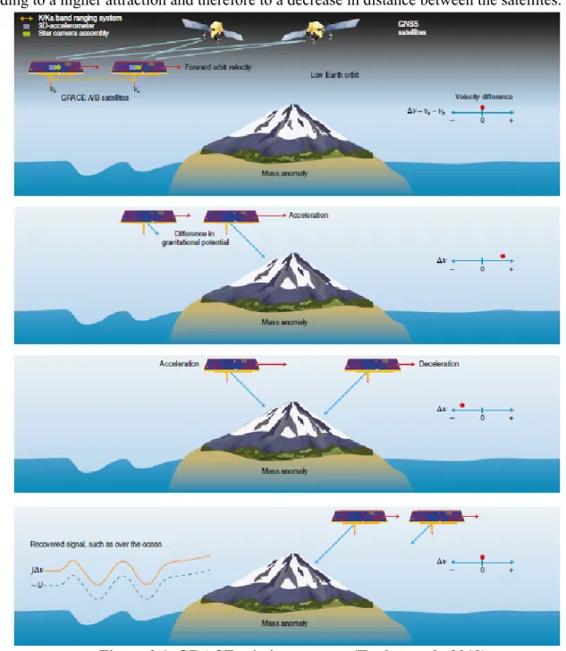
The general concept of GRACE satellite measurements flying at low altitudes with satellite to satellite tracking originated from a methodology proposed by Wolff (1969) for obtaining a more accurate gravity field model (Figure 2.1). Gravitational variation in the Earth’s gravity field influence the distance between twin satellites. For instance, if the leading satellite passes over areas

(41)

of stronger gravity, i.e, greater mass concentration, the change in the gravitational field increases the distance between the two satellites. Then, the tailing satellite approaches the gravity anomaly, leading to a higher attraction and therefore to a decrease in distance between the satellites.

Figure 2.1. GRACE mission concept (Tapley et al., 2019).

Small changes in the distance between the two satellites are measured using a K-band Ranging system (Tapley et al., 2004b). This ranging system can detect changes in separation distance between two GRACE satellites within one micron by using the dual-frequency one-way of K- and Ka-band phase measurement transmitted and received by both satellites (Dunn et al., 2003).

(42)

GRACE-FO as a rebuild of the GRACE mission is equipped with microwave ranging for measuring changes of intersatellite distance, and a laser ranging interferometer (LRI) as a demonstrator experiment (Sheard et al., 2012). A design precision of laser interferometry is approximately 26 times better than the K-band ranging system and it is expected to increase the accuracy of measurements by tenfold or more (Tapley et al., 2019). Furthermore, the position and timing of satellites with an accuracy of centimeter is determined with the Global Positioning System (GPS). The non-gravitational forces acting on satellites are removed from along-track observations using the precise accelerometers to make sure that only accelerations caused by gravity are considered in the distance measurements (Tapley et al., 2004b). The precise attitude estimations of inertial orientation for the GRACE satellites are determined using star camera assembly.

2.1.2. GRACE science data

The GRACE Science Data System (SDS) distributes monthly gravity field processing for both GRACE and GRACE-FO missions through all tasks required for the production of the monthly and mean gravity field solutions (Figure 2.2). The monthly satellite gravimetric solutions are found in the Jet Propulsion Laboratory (JPL), the Center for Space Research (CSR) of the University of Texas at Austin, and the GeoforschungsZentrum Potsdam (GFZ) of Germany. Each center uses parameter choices and solution strategies to convert relative ranging observations between twin satellites to gravity changes (Bettadpur, 2012).

Both GRACE and GRACE-FO data products appear at different levels, including, 1, level-2, and level-3 processing. The level-1 is as a result of the irreversible processing steps applied to GRACE and GRACE-FO raw data. In level-1 products, the data sample rate is reduced and data are time-tagged to the respective satellite receiver clock time. The Level-1 data include the ancillary data products required for further processing (Bettadpur, 2012). GRACE and GRACE-FO level-2 time-variable gravity field data consist of a set of normalized geopotential spherical harmonic coefficients or more recently as gridded mascon (mass concentration blocks, Watkins et al., 2015). The geopotential term is referred to the exterior potential of the Earth system including the entire solid and fluid (ocean and atmosphere) compartments (Bettadpur, 2018). Following the conventional methods (Heiskanen and Moritz, 1967), the gravitational potential attraction between

(43)

a unit mass and the Earth System can be expressed in terms of spherical harmonic expansion as : 𝑉(𝜆, 𝜃, 𝑟) = 𝐺𝑀 𝑅 ∑ ( 𝑅 𝑟) 𝑙+1 ∑ 𝑃̅𝑙𝑚(cos 𝜃) 𝑙 𝑚=0 𝑙_𝑚𝑎𝑥 𝑙=0 [𝐶𝑙𝑚cos(𝑚𝜆) + 𝑆𝑙𝑚sin(𝑚𝜆)] (2.1)

Figure 2.2. GRACE and GRACE-FO mission data flow (Cooley and Landerer, 2019).

Where Clm and Slm are fully normalized spherical harmonic coefficients of degree l and order m,

𝑃̅_𝑙𝑚 are fully normalized associated Legendre functions of degree l and order m, M is the total mass of the Earth (kg), G is Newton's gravitational constant (m3_{/(kg s}2_{)), R (m) is the Earth’s radius, and}