Imaging the Main Frontal Thrust in Southern Bhutan using high-resolution near-surface geophysical techniques : implications for tectonic geomorphology and seismic hazard assessment

(1)

HAL Id: tel-01693914

https://tel.archives-ouvertes.fr/tel-01693914

Submitted on 26 Jan 2018

HAL is a multi-disciplinary open access archive for the deposit and dissemination of sci-entific research documents, whether they are pub-lished or not. The documents may come from teaching and research institutions in France or abroad, or from public or private research centers.

L’archive ouverte pluridisciplinaire HAL, est destinée au dépôt et à la diffusion de documents scientifiques de niveau recherche, publiés ou non, émanant des établissements d’enseignement et de recherche français ou étrangers, des laboratoires publics ou privés.

Imaging the Main Frontal Thrust in Southern Bhutan

using high-resolution near-surface geophysical

techniques : implications for tectonic geomorphology and

seismic hazard assessment

Dowchu Drukpa

To cite this version:

Dowchu Drukpa. Imaging the Main Frontal Thrust in Southern Bhutan using high-resolution near-surface geophysical techniques : implications for tectonic geomorphology and seismic hazard assess-ment. Earth Sciences. Université Montpellier, 2017. English. �NNT : 2017MONTT101�. �tel-01693914�

(2)

UNIVERSITÉ DE MONTPELLIER

ECOLE DOCTORALE SIBAGHE

THESIS

To obtain the title of

PhD of Science of the University of Montpellier

Speciality: Geophysics, Seismology and Geology

I

MAGING THE

M

AIN

F

RONTAL

T

HRUST IN SOUTHERN

B

HUTAN

USING HIGH

-

RESOLUTION NEAR

-

SURFACE GEOPHYSICAL

TECHNIQUES

: I

MPLICATIONS FOR TECTONIC GEOMORPHOLOGY

AND SEISMIC HAZARD ASSESSMENT

Defended by :

Dowchu D

RUKPA

Thesis defense committtee members

CATTIN Rodolphe Geosciences Montpellier Directeur de thèse GAUTIER Stéphanie Geosciences Montpellier Directeur de thèse GIRARD Jean-Francois EOST-Univ. Strasbourg Président

HETÉNYI György Univ. Lausanne Rapporteur

BOLLINGER Laurent CEA Examinateur

BODET Ludovic McF METIS-Univ. Paris 6 Examinateur

(3)

(4)

i

Abstract

Recent studies in southern-central Bhutan have proposed a Holocene slip rate of 20.8±8.8 mm/year. This overthrusting slip rate is estimated based on a mean vertical uplift rate of 8.8±2.1 mm/year and assuming a constant frontal thrust dip angle of 25◦_±5◦ _extrapolated

from structural measurements. Since geometry of the fault is a key parameter for discerning the slip rate and its associated seismic hazard assessment, we employed near-surface geo-physical approach to accurately constrain the Topographic Frontal Thrust (TFT) geometry at shallow depth. Based on proven effectiveness of near-surface geophysical techniques for studying active faults, we adopted gravity, seismic and electrical resistivity tomography.

We deployed geophysical profiles at three key sites along the southern frontal areas of the Bhutan Himalayas. The first study area is in Sarpang, a small town located in southern-central Bhutan where we performed all three geophysical methods adopted. The second site is located in Phuentsholing in the south-western Bhutan, where we performed gravity and electrical resistivity survey. The third site is located between Sarpang and Phuentsholing, in the sub-district of Lhamoizingkha under Dagana district. A stochastic inversion approach was adopted to perform analysis of geophysical data collected from the above sites expect for Lhamoizingkha area. Unlike commonly used approaches based on search for the simplest model, the main advantages of this approach include its ability (1) to assess the fault ge-ometry because no smoothing is applied, (2) to provide a measurement of the uncertainties on the obtained dip angle and (3) to allow trade-off analysis between geometric and either electrical resistivity, velocity or density properties.

The stochastic inversion results from Sarpang site show a TFT that is characterized by a flat and listric-ramp geometry with a north dipping dip angle of ca. 20◦_-30◦ _{at the upper}

depth of 0-5 m, steeply dipping angle of 70◦ _{in the middle 5-40 m depth and flattening with}

a dip angle of 20◦ _{at deeper depths. These new results allow us to estimate a minimum}

overthrusting slip rate of 10±2 mm/year on the TFT, which is about 60% of the far-field GPS convergence rate of ca. 17 mm/year. Based on these constraints we propose that, in Sarpang site, significant deformation partitioning on different faults including the TFT, the Main Boundary Thrust (MBT) and the Frontal Back Thrust (FBT) cannot be ruled out. More importantly, assuming a constant slip rate, the dip angle variations constrained from the present study correspond to variations in the deduced uplift rate with distance from the TFT. This, therefore, emphasizes the drawbacks in assuming constant dip angle measured

(5)

ii

from surface observations and uplift rate estimates based on terrace dating only at the front, which may significantly bias the slip rate estimation.

Unlike in Sarpang, the TFT corresponds to the Main Frontal Thrust (MFT) in Phuentshol-ing. At this site a preliminary study suggests a MFT characterized by a flat and listric-ramp geometry. With additional terrace dating information, slip rate for the Phuentsholing area will be performed in a near future. Overall based on the stochastic inversion results, we pro-pose a MFT geometry similar to that observed in Sarpang but with possible lateral variations in terms of deformation partitioning. In Lhamoizingkha area, the exact location of the MFT is not known. Our preliminary results suggest a complex fault trace and indicate that the MFT is located further north of the current resistivity line deployed in this area. Similar to Phuentsholing site (but contrary to Sarpang), we observed that the MFT is the most frontal structure and therefore most of the convergence in the area could be accommodated by the MFT, which is also in agreement with GPS observations.

(6)

iii

Résumé

Des études récentes menées dans la région de Sarpang au sud du centre du Bhoutan es-timent un taux de glissement Holocène de 20,8± 8,8 mm/an sur le «chevauchement frontal himalayen» est utilisé pour le MFT, pas le TFT.Que diriezvous de «chevauchement au front topographique »? Plus bas : effacer l’espace entre «au-del » et «à». Cette valeur est basée sur un taux de surrection moyen mesuré de 8,8± 2,1 mm/an et en supposant pour ce chevauche-ment un pendage constant de 25◦ _{± 5}◦_{. La géométrie des failles est un paramètre clé dans}

l’estimation de la vitesse de glissement et donc dans l’évaluation de l’aléa sismique. Dans le cadre de ce travail, nous avons utilisé une approche géophysique de proche surface afin d’estimer précisément la géométrie de ce chevauchement.

Nous avons déployé des profils géophysiques dans trois sites clés le long de la frontiére sud du Bhoutan. La première zone d’étude se trouve à Sarpang, une petite ville située au centre du Bhoutan où nous avons effectué des mesures gravimétriques, sismiques et électriques. Le deuxième site est situé à Phuentsholing dans le sud-ouest du Bhoutan, où nous avons effectué des mesures gravimétriques et de résistivité électrique. Le troisième site est situé entre Sarpang et Phuentsholing, à Lhamoizingkha dans le district de Dagana.

Excepté pour la région de Lhamoizingkha, une approche d’inversion stochastique a été adoptée pour analyser des données géophysiques collectées. Contrairement aux approches couramment utilisées basées sur la recherche du modéle le plus simple, les principaux avan-tages de cette approche sont sa capacité (1) à mieux estimer la géométrie des zones de discontinuité car aucun lissage n’est appliqué, (2) à fournir une mesure des incertitudes sur le pendage obtenu et (3) à permettre une analyse des relations possibles entre les propriétés géométriques et celles du milieu (résistivité électrique, vitesse ou densité).

Les résultats d’inversion stochastique du site de Sarpang montrent un TFT qui se carac-térise par une géométrie en plat-rampe-plat avec un pendage vers le nord d’environ 20◦_-30◦

dans la partie la plus superficielle (profondeur < 5 m), un pendage fort de 70◦ _{entre 5 m}

et 40 m de profondeur et un l’aplatissement avec un pendage de 20◦ _{au-del à de 40 m.}

Ces nouveaux résultats nous permettent d’estimer un taux minimal de glissement de 10 ± 2 mm/an sur le TFT, soit environ 60% des 17 mm/an associés au taux de convergence GPS moyen obtenu en champ lointain. Sur la base de ces contraintes, il apparait donc qu’on ne puisse pas exclure la possibilité que la déformation soit distribuée sur plusieurs failles, comprenant le TFT, mais également d’autres chevauchements comme le MBT (au nord) ou

(7)

iv

le FBT (au sud). De plus, en supposant un taux de glissement constant, les variations de pendage obtenues induisent des variations du taux de surrection en fonction de la distance au TFT. Cela souligne les faiblesses des hypothèses couramment faites pour estimer les taux de glissement Holocène sur les failles sismogènes : (1) pendage constant estimé uniquement à partir des observations de surface et (2) estimations du taux de surrection en supposant une surrection identique pour une terrasse fluviale donnée.

Contrairement à Sarpang, à Phuentsholing le TFT correspond au chevauchement frontal himalayen (MFT). Sur ce site, l’étude préliminaire que nous avons menée suggère un MFT ayant une gèomètrie de faille listrique. Des mesures de datations doivent maintenant être effectuées pour estimer le taux de glissement sur le MFT dans cette zone. Dans la région de Lhamoizingkha, l’emplacement exact du MFT n’est pas connu. Nos résultats préliminaires suggèrent une géométrie complexe de la trace de la faille en surface et indiquent que le MFT est situé plus au nord de la ligne de résistivité déployée dans cette zone. À l’instar du site de Phuentsholing (mais contrairement à Sarpang), nous avons observé que le MFT était la structure la plus frontale et que l’essentiel de la convergence dans cette zone pouvait être accommodé par le MFT, comme semble le suggérer les observations GPS.

(8)

v

Acknowledgments

Every pursuit to accomplish important milestones in life become possible when the pro-cesses to realize the end goal is supported and driven by great mind with ultimate objective to advance knowledge for the betterment of the society that we live in. Nothing more and nothing less!

My scientific curiosity and professional interest takes me to the University of Montpellier (France) to pursue Doctor of Philosophy in Geosciences at the beginning of 2015. The idea of doing a PhD was conceived when I met Rodolphe Cattin in 2010 while conducting gravity study in Bhutan as part of cooperation research project between the Department of Geology and Mines, Geosciences Montpellier (University of Montpellier) and ETH Zurich. In the years that ensued, we jointly developed a project proposal on“Seismic coupling and megaquake along the Himalayan arc”. Unfortunately, the proposal didn’t get approved until mid-2014

after three successive resubmissions. Immediately upon approval of the project by theFrench Agence Nationale de la Recherche (ANR), Rodolphe informed me about the good news

and also reminded me about the prospect of starting my PhD. I was overjoyed and at the same time intimated by the enormity of commitment required to accomplish such a major undertaking in my life. I immediately replied to Rodolphe asking for some time to discuss with my family and get back to him with a decision. It was indeed a tough decision for me, especially realizing full well that pursuing a PhD would require me to be away from my family for a longer period of time. But in the end with full support my family and out of my own interest, I decided to undertake PhD study knowing full well, the challenges and commitment that I have to endure over the next three years.

Three years have now gone by and I have sacrificed a good amount of my time and energy in what I believe will make an important contribution in understanding the science and in enhancing my capacity as an individual. In this context, I must first of all sincerely thank Professor Rodolphe Cattin for giving me this unforgettable opportunity, and more

importantly, for believing in me and rendering your unfailing support throughout the last three years. I am highly indebted to you and I shall never forget your kindness and for being always there when ever I needed your help. My sincere thanks toStéphanie Gautier for your

amazing support and I was indeed fortunate to have you as my co-supervisor. Your words of encouragement and critical comments helped me a great deal to complete this thesis. Thanks again for everything to both Rodolphe and Stéphanie!

(9)

vi

My sincere thanks to comity membersLudovic Bodet and Marguerite Godard and thesis

defense committee members:Rodolphe Cattin, Stéphanie Gautier, Jean-Francois Girard, György Hetényi, Laurent Bollinger and Ludovic Bodic for sparing their time and providing

insightful comments. I must particularly thankGyörgy for thorough review of the draft thesis

and providing invaluable comments, which greatly improved this manuscript.

My thanks also goes to amazing friends at Geosciences Montpellier including Jeff Ritz, Matthieu Ferry, Romain Le Roux-Mallouf and Stéphane Mazzotti with whom I had great

opportunity to associate with both in Montpellier and during the field works in Bhutan. I will cherish the good moments we had together. Thanks also toTheo Berthet for permitting me to

use his LA_{TEX code, which really helped me in writing and compilation of this thesis. I must also}

sincerely acknowledge my colleagues in DGM who helped us in deployment of geophysical investigation in southern Bhutan. Without their help, it would have been extremely difficult to accomplish the data acquisition task.

Last but not the least, I sincerely thank my beautiful and loving wife,Tshering Denka for

her understanding and taking good care of our most adorable son, Jigmi Namgyel Yoezer.

Without my wife’s understanding and support, I will not have been able to complete my PhD. I owe you a lot now and forever!

This research thesis was funded byFrench Agence Nationale de la Recherche (ANR-13-BS06-006-01).

(10)

LIST OF FIGURES

2.1 Cartoon depicting the Tethys sea that separates India from Eurasia during pre-Valanginian time, gradual subduction of the Tethys along the southern margin of Asia and collision of the two continents leading to formation of the great Himalayas (After Avouac, 2008). . . 8

2.2 (a) Simplified geological map of the Himalayan arc, (b) Cross-section along AA’ in (a) along the longitude of Katmandu.Thick black line represents the MHT which expresses at the the surface as MFT at the front of the Siwalik Formation (Modified after Avouac, 2008). . . 10

2.3 Wide-angle seismic data showing variation in the depth of reflections coming from Moho underneath the Higher Himalayas and south of Yarlung Tsangpo (After Hirn et al, 1984). . . 13

2.4 Reflections from the INDEPTH deep seismic profile and corresponding inter-preted major tectonic features MHT, STD and Moho (After Zhao et al, 1993). 14

2.5 Interpretative cross-section of India-Eurasia collision zone. The Indian litho-sphere underplates the Himalaya and Tibetan plateau upto∼450 km from the MFT (After Hetényi, 2007). . . 15

2.6 Arc-Parallel Gravity Anomaly. Red and blue values represent higher and lower values of gravity, resepectively, compared to the average profile perpendicular to the Himalayan arc. Yellow lines show change in arc-parallel gravity anomaly and highlight segments (After Hétenyi et al., 2016). . . 17

(11)

viii List of Figures

2.7 Coupling model and fit to the horizontal GPS data. Interseismic area is shown as shades of red. A coupling value of 1 means fully locked and 0 means fully creeping. The green and black arrows show the continuous and campaign gps velocities with their error bars, respectively. The blue arrows shows the mod-eled velocities which fit with the coupling. The dashed-line shows separation of region within which the long term velocity for that region is calculated show by large red arrow (After Stevens and Avouac, 2015). . . 18

2.8 Mid-crustal microseismicity from 1996-2008 superimposed on shear stress ac-cumulation rate on MHT, deduced from coupling pattern. The red line shows the 3500 m elevation beyond which the seismicity seems to drop (After Ader et al., 2012). . . 19

2.9 Interseismic coupling of the MHT in the Bhutan Himalayas. Rectangles show interseismic coupling for different fault segments. The hatched segment rep-resents flat part of the MHT. Colored base map reprep-resents coupling as shown in Figure 2.7. Dashed blue line shows the possible limits of the fully coupled zone.Green triangles show GPS station and black triangles represents GPS sta-tions used in Stevens and Avouac, 2015 (After Marechal et al., 2016).. . . 20

2.10 (a) Seismicity of the Himalayan region showing location of events that oc-curred between 1961-1981. Large, medium and small circles show very good, good and fair quality of epicenter location on basis of station locations and travel time residuals. Most of the epicenters lie along a relatively narrow belt of about 50 km between MCT and MBT. Seismicity within the triangles (A, B, C, D, E) are projected linearly on the center line of each triangle. (b) Fault plane solutions of historical events showing mostly compressional regime (Af-ter Ni and Barazangi, 1984).. . . 21

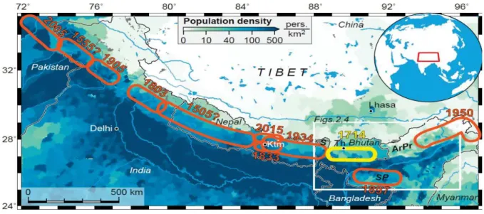
2.11 Observations and model results related to the 1714 earthquake in the Bhutan Himalayas. Grey star and circle indicate, respectively, the location and in-tensity of earthquake as reported by Ambraseys and Jackson[2003] Abbre-viations: WP-Wangdue Phodrang, Ga-Gangteng Monastery, Sa-Sarpang, Ge-Gelephu, Ba-Bahgara, Ch-Charaideo Hill, Ti-Tinkhong, pOF-proposed Oldham Fault, DF-Dauki Fault. Cities: Th-Thimphu, Da-Darjeeling, Gu-Guwahati, Te-Tezpur, Sh-Shillong, Jo-Jorhat (After Hetényi et al., 2016). . . 24

(12)

List of Figures ix

2.12 Great earthquakes along the Himalayan arc since 1500 AD (After Hetényi et al. 2016). . . 25

2.13 Synthesis of paleoseismic records along the Himalayas (a). Synoptic calen-der and locations of great/large earthquakes along the Himalayan front. Grey bars indicate minimum source lengths with or without observed surface rup-ture. Vertical orange bars show radio-carbon model constrains on the timing of different events. Vertical orange bars show the ∼ 3500 year long record deduced from Piping area (Le Roux-Mallouf et al., submitted). . . 26

3.1 Common geometric configurations used in electrical resistivity survey . . . 37

3.2 The resistivity of rocks, soils and minerals (After Loke, 2015) . . . 40

3.3 Flow chart to characterize fault activity in Quaternary settings for engineering applications (After Suzuki et al. 2000). . . 42

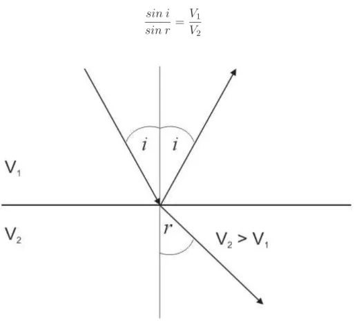
3.4 Relationship between angle of incidence(i) and angle of refraction (r) in layers with velocityV1 andV2 where V2 > V1. . . 43

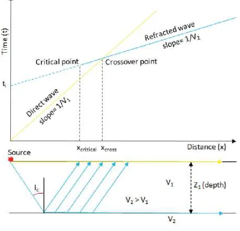
3.5 Travel-time curves for the direct wave and head wave from a single refractor. 45

3.6 Travel-time curves for the head wave arrivals from a dipping interface in for-ward and reserve directions along a refraction profile (top); Ray-path geome-try (Modified after Kearey, 2013) . . . 46

3.7 Schematic diagram showing the relationship between model and data . . . . 53

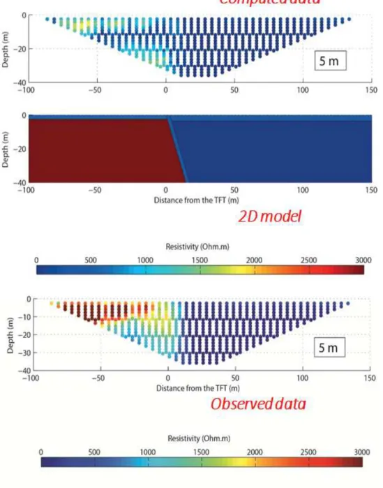
3.8 A 2D best fit model obtained by comparing the synthetically computed data with the observed data and applying stochastic inversion processes. . . 58

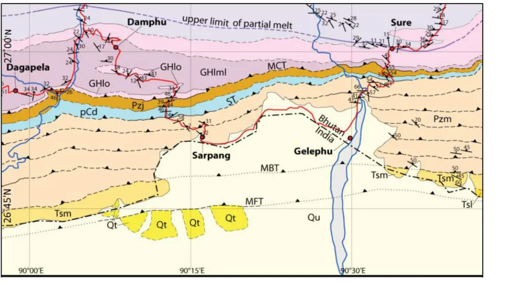
4.1 Map of Sarpang area showing the major geological and tectonic units (Abbre-viation in the map: Qt-River terraces; Qu-Unconsolidated sediments deposited in braided stream;Tsl-Lower member Siwalik Group; Tsm-Middle member Si-walik Group; Pzm-Manas Formation; Pzj-Jaishidanda Formation; pCd-Daling Formation; GHlo-Greater Himalaya structurally lower orthogneiss unit; GHlml-Greater Himalaya structurally lower metasedimentary unit; MFT-Main Frontal Thrust; MBT-Main Boundary Thrust; ST-Shumar Thrust; MCT-Main Central Thrust (After Long et al., 2011).. . . 63

(13)

x List of Figures

4.2 Geomorphological map of Sarpang area. (a) Shaded map of Sarpang showing the location of MFT and TFT. Black triangle shows the location of study area. (b) Geomorphological map of TFT in Sarpang superimposed on Pleiades DEM. Alluvial terraces are labeled TO (active channel) to T6 (oldest). Blue triangle represent location of paleoseismic trench. Black points show elevation from Pleiades DEM with countour interval of 20 m (After Le Roux-Mallouf et al., 2016). . . 64

4.3 Detailed log over a 2 m grid at the paleoseismic trench in Sarpang showing major geological and tectonics units. The solid and dashed red lines show the main certain and suspected faults, respectively. Thick black lines labeled EH 1 and EH 2 denote the event horizons. (After Le Roux-Mallouf et al., 2016). . . 65

4.4 1 m spacing Dipole-Dipole model generated using res2dmod involving 2 layers with high resistivity contrast and gently dipping TFT. . . 68

4.5 Inversion model resistivity section obtained using data generated from the model in Figure 4.4. . . 68

4.6 Location of electrical resistivity line with respect to the position of the fault and paleoseismic trench. . . 69

4.7 2D Dipole-dipole array ERT section with 1 m (top), 2.5 m (middle) and 5 m (top) electrode spacing . . . 74

4.8 2D Wenner-Schlumberger array ERT section with 1m (top), 2.5 m (middle) and 5 m (top) electrode spacing . . . 75

4.9 Schematic diagram of the finite difference or finite element used in the res2dmod program (After Loke, 2015). . . 76

4.10 Simplified geometry of the subsurface used in the forward modeling process . 77

4.11 Results of the forward model using res2dmod to test the effect of different layers (a) ERT pseudo-section with 5 m interval obtained from observed data (b) 3 layers model with 5 m interval and TFT dip angle of 40◦ _{(c)4 layers}

model with 5 m interval and same TFT dip angle (d) 5 layers model with 5 m interval and same TFT dip angle. . . 78

4.12 Effect of mesh on the model resistivity output . . . 80

4.13 The best fit resistivity value obtained for SL and NL layers defined in Figure 4.10 81

(14)

List of Figures xi

4.15 The best fit thickness and resistivity value for the fault zone defined in Figure 4.10 . . . 82

4.16 Layout plan for acquisition of seismic data along the profile. The TFT location at the mid-point of profile 2 is shown with red arrow. . . 83

4.17 First arrival travel-time picks for all in-line shots along the seismic refraction profile . . . 85

4.18 Comparison of first arrival travel-time picks between three pickers. . . 86

4.19 Shot location along the study seismic profile. Color scale indicates first arrival travel-time from each shot location to the geophone positions along the profile. 87

4.20 Tomographic image showing velocity variation on both sides of the TFT. . . . 89

4.21 Ray coverage illustrating the area resolved in tomographic inversion in Figure 4.20. The TFT is located around the 0 m distance. . . 89

4.22 Measured gravity (top), elevation (middle) and gravity variations corrected for both topographic effect and regional trend (bottom) along the study profile. Data uncertainty is associated with both accuracy of the CG5 gravimeter and error in elevation measurement.. . . 92

5.1 Location map showing the geophysical study area in Phuentsholing, Lhamoiz-ingkha and Sarpang . . . 150

5.2 Three sites located using google Earth image for reconnaissance study and detailed geophysical investigation. . . 151

5.3 Thick alluvial fan deposit at the foothills of Site 3. . . 152

5.4 Panoramic view at site 1 showing formation of three levels of terraces as result of repeated tectonic uplift. . . 152

5.5 Location of drill bore-holes (BH-01 and BH-02) and geophysics line (yellow line) in Phuentsholing at Site 1. Inset picture shows drilling work in process at BH-02. . . 153

5.6 Drill core from BH-01 and BH-02. Red rectangle shows the dark, non-cohesive and unconsolidated materials observed between∼13-18 m at BH-01. . . 153

5.7 Description of core-log lithology from drill bore-holes, BH-01 and BH-02. . . . 154

5.8 (A) Epicenter location with pattern of linear seismicity corresponding to the Goalpara lineament (Velasco et al., 2007); (B) Major active fault zones imaged by GANSSER project seismic catalog showing the prominent dextral Dhubri-Chungthang Fault zone (After Diehl et al., 2017). . . 156

(15)

xii List of Figures

5.9 Distribution of geomorphologic surfaces and active faults. Red square shows location of our Site 1 in Phuentsholing (After Yagi et al, 2002). . . 157

5.10 Structural attitudes of geological outcrops in Phuentsholing and vicinity area. Inset picture shows steeping dipping highly sheared phyllite in-situ exposure at Site 1. . . 158

5.11 Observed Wenner-Schulumberger ERT pseudo-section with varying current in-tensity . . . 160

5.12 Dipole-Dipole (top) and Wenner-Schulumberger (bottom) ERT pseudo-sections obtained using 8 mA current injection. . . 163

5.16 Measured gravity data (a), elevation (b) and topographic corrected gravity variations along the profile (c). The drill bore-hole (BH-01) is located between 66-72 m along the profile. . . 168

5.17 Geometry of the model used in the stochastic inversion. STL - South Top layer, NTL - North Top Layer, SL - South Layer and NL - North Layer. xfault is the possible location of the fault on the surface with respect to fault gouge ob-served in bore-hole at ca. 13-18 m depth and resistivity distribution in the subsurface. Model thickness is associated with the thickness investigated by each geophysical method. . . 170

5.18 Distribution of MFT angle from ERT sections using Wenner-Schulumberger array with different amount of current injection . . . 171

5.19 Distribution of MFT angle from Wenner-Schlumberger ERT sections by com-bining PHUN2, PHUN3, PHUN4 and PHUN5 shown in Figure 5.19 . . . 171

5.20 Bivariate frequency histograms between dip angle and other parameters of the ERT model obtained using Wenner-Schulumberger array . . . 172

(16)

List of Figures xiii

5.21 Observed and Calculated Wenner-Schlumberger array and the optimal misfit between Observed and calculated ERT sections that correspond to obtained MFT geometry and petro-physical characteristics. The red rectangle in the model section indicates the location of drill borehole, BH-01. . . 174

5.22 Comparison between observed (blue circles) and calculated (dark green lines) gravity variations along profile line for 100 best fitting models (top); Density contrast models without drill borehole information but with different SL and NL thickness(Bottom). . . 175

5.23 Distribution of MFT dip angle from gravity measurements without incorporat-ing bore-hole information in the inversion process. . . 176

5.24 Relationship between the obtained dip angle and the other parameters of the density model. Note that density means density contrast with respect to den-sity of the North top layer. . . 177

5.25 Comparision between observed (blue circles) and calculated (dark green lines) gravity variations along profile line for 100 best fitting models (top); Density contrast models with drill bore-hole information and with varying SL and NL thickness(bottom). . . 179

5.26 Distribution of MFT dip angle from gravity measurements with inclusion of drill bore-hole information in the inversion process. . . 180

5.27 Relationship between the obtained dip angle and the other parameters of the density model. Note that density means density contrast with respect to den-sity of the North top layer. . . 181

5.28 (a) Topographical map of Bhutan showing the location of the Lhamoizingkha region . (b) The Lhamoizingkha and vicinity areas show markers indicating intense tectonic activity: a system of perched alluvial terraces, landslides and evidences of surface rupture of the MFT. The black boxes show the location of the different paleoseismic study sites and red box at Chokott Creek is location where geophysical study was performed (Modified from Le Roux-Mallouf, 2016).184

5.29 Location of the Piping paleoseismic trench on the left bank of Wang Chhu. . . 185

5.30 Geological map of the Piping-Lhamoizingkha area (After Le-Roux Mallouf, 2016).186

5.31 Diagram showing how ZZ FlashRes resistivity collects data compared to con-ventional resistivity equipment. . . 187

(17)

xiv List of Figures

5.33 Electrical resistivity profile line in relation to the inferred MFT and power line 188

5.34 ERT section for 1m electrode spacing using Dipole-Dipole (top) and Wenner (bottom) geometric configuration . . . 190

5.35 ERT section for 2.5 m electrode spacing using Dipole-Dipole (top) and Wenner (bottom) geometric configuration . . . 191

5.36 ERT section for 5 m electrode spacing using Schlumberger (top) and Wenner (bottom) geometric configuration . . . 192

5.37 Location of paleoseismic trench, MFT and proposed geophysical line in Piping area. . . 194

6.1 Profiles of elevation and slope for 50 km-wide swaths in Nepal (A) and Bhutan (B). Values sampled every 5 km along swath; maximum, minimum, and mean elevations and slopes are for each 5 × 50 km rectangle along swath. Relief computed as standard deviation of elevations. Gray scale shading between maximum and minimum swath elevations is density plot (histogram) of tion samples (darker indicates greater concentration of terrain at that eleva-tion). C-F: Comparison of Nepal and Bhutan profiles aligned at high peaks and Main Frontal thrust. Heavy vertical line at position of high peaks; thin solid (Nepal) and dashed (Bhutan) vertical lines are where profiles cross 2 km or 1 km elevations (dotted horizontal lines) (After Duncan et al., 2003). . . 197

6.2 Topographic and precipitation profiles, in 40-km-wide swaths, across Bhutan Himalayas and Shillong plateau show that an orographic barrier of 1.5-2 km is sufficient to hinder moisture transport. A-eastern Bhutan; B-western Bhutan. Topography (orange) has been derived from Shuttle Radar Topography Mis-sion data; precipitation (blue) is taken from the calibrated Tropical Rainfall Measuring Mission data. There is a strong E-W precipitation gradient: at ∼ 1-1.5 km elevation in the east it is ∼ 4 m/yr, while in the west it is ∼ 6 m/yr. MFT–Main Frontal thrust, MBT–Main Boundary thrust, MCT–Main Cen-tral thrust, KT–Kakhtang thrust, STD–South Tibetan detachment, LHS–Lesser Himalayan Sequence, GHS–Greater Himalayan Sequence, TK–Tethyan Klip-pen, PW–Paro window, TSS–Tethyan Sedimentary Sequence (After Grujic et al., 2006). . . 200

(18)

List of Figures xv

6.3 Interseismic coupling of the Main Himalayan Thrust in Bhutan. Rectangles show our estimates of interseismic coupling for the different fault segments. The hatched segment represents the flat part of the MHT constrained by the inversion. The colored base map representing seismic coupling estimates and black triangles representing GPS stations are from Stevens and Avouac (2015). Dashed blue lines show the possible limits of the fully coupled zone. Green triangles show the locations of our new GPS stations. (After Marechal et al., 2017). . . 201

6.4 Tectonics models showing the role of Indian crust in collision dyanamics of western and eastern Bhutan (After Singer et al., 2017). . . 202

6.5 Seismotectonic model of the Bhutan Himalayas and its link to the foreland deformation. (After Diehl et al., 2016). . . 203

7.1 Estimated slip rate inferred from both fault geometry and observed uplift rate. (a) Uplift rate along the study profile. Red and green curves are show two end-member models obtained for fault geometry. Thick blue line denotes the far-field shortening rate estimated from GPS measurements (Marechal et al., 2016). It corresponds to the upper limit of uplift rate, which can be associated with a theoretical vertical fault. Gray circle is the observed uplift rate assum-ing a northward distance of 5 m from the TFT as reported by Berthet et al., 2014. (b) Same as (a) except a northward distance of 10 m is assumed. (c) Estimated slip along the TFT at depth assuming a constant uplift rate along the study profile for the two-end member models denoted by red and green curves. Hatched area around the curves is associated with uplift rate uncer-tainties. The thick grey dashed lines point out the area of uplift rate assuming a northward distance from the TFT of 5 m and 10 m, respectively. Note that within this area, the uncertainties in the uplift rate spikes up close to the TFT and decreases away from the front towards the north. Thick blue line denotes the far-field shortening rate estimated from GPS measurements (Marechal et al., 2016), which is the upper limit of slip rate. The slip obtained from rigid blocks model with a constant dip angles ranging from 10◦ _{to 60}◦ _{is given by}

(19)

(20)

LIST OF TABLES

4.1 List of geophysical equipments used in 2015 field survey . . . 67

4.2 GPS coordinates along the electrical resistivity profile with 5m electrode spac-ing in Sarpang . . . 70

4.3 Range of a priori geophysical parameters used in res2dmod . . . 79

5.1 List of geophysical equipments for geophysical field survey in Phuentsholing . 150

5.2 Inversion results. The parameter values are associated with the most high-est relative frequency model. The associated uncertainties are indicated in bracket. Uncertainties on each parameter are given by the full width at half maximum. The symbol ‘-’ means no constraint has been obtained. . . 173

(21)

(22)

I

Methods

27

3 Near-surface geophysics 29

3.2 Advantages and shortfalls of near-surface geophysical methods . . . 30

3.3 Types of geophysical methods . . . 31

3.3.1 Electrical resistivity . . . 32

(23)

xx TABLE OF CONTENTS

3.3.3 Gravity . . . 48

3.4 Geophysical Inverse theory . . . 52

3.4.1 Conceptual Introduction . . . 52

3.4.2 Mathematical background . . . 54

3.4.3 Stochastic Inversion used in the thesis . . . 56

II

Application to south-central and south-west Bhutan

59

4 Characterization of Topographic Frontal Thrust geometry in Sarpang 61

4.1 Geology of study area . . . 61

4.1.1 Introduction . . . 61

4.1.2 Geology and tectonics . . . 61

4.1.3 The Topographic Frontal Thrust (TFT) . . . 62

4.2 Geophysical field campaign 2015 . . . 65

4.2.2 Schedule of field program . . . 66

4.2.3 List of field equipments . . . 67

4.2.4 Electrical Resistivity Profile . . . 67

4.2.5 Seismic refraction . . . 83

4.2.6 Micro-gravity . . . 90

4.2.7 Results, discussion and conclusion: GJI paper . . . 93

5 Main Frontal Thrust geometry in Phuentsholing and Lhamoizingkha: Preliminary

results 149

5.2 Field work in Phuentsholing in 2016 . . . 149

5.2.1 List of field equipments . . . 150

5.2.2 Site selection . . . 150

5.3 Geology of study area . . . 155

5.4 Data acquisition. . . 159

5.4.1 Electrical Resistivity and gravity data . . . 159

5.5 Data analysis . . . 161

5.5.1 Electrical resistivity tomography . . . 161

5.5.2 Gravity . . . 167

(24)

TABLE OF CONTENTS xxi

5.6.1 Results . . . 169

5.6.2 Discussion and conclusions . . . 179

5.7 Field work in Lhamoizingkha . . . 183

5.7.2 Geology of Piping-Lhamoizingkha area . . . 185

5.7.3 Field equipment . . . 187

5.7.4 Electrical resistivity data . . . 187

5.7.5 Conclusion . . . 193

6 Lateral variations along the Himalayan arc 195

6.2 Lateral variations: Bhutan Himalayas vs Nepal Himalayas . . . 196

6.3 Lateral variations across the Bhutan Himalayas . . . 198

6.3.1 Geology, topography& seismotectonics . . . 198

6.3.2 Geometry of the MFT . . . 204

6.4 Conclusion . . . 205

7 Conclusions 207

7.1 Main results . . . 207

7.2 Discussions . . . 210

7.2.1 Overthrusting slip rate estimation . . . 210

7.2.2 Tectonic deformation at the front . . . 213

7.3 Future works . . . 214

References. . . 217

A Annexes 233

A.1 First paleoseismic evidence for great surface-rupturing earthquakes in the Bhutan Himalayas . . . 233

A.2 Evidence of interseismic coupling variations along the Bhutan Himalayan arc from new GPS data . . . 247

A.3 Segmentation of the Himalayas as revealed by arc-parallel gravity anomalies . 265

(25)

(26)

❈❍❆#❚❊❘

✶

INTRODUCTION: THESIS OVERVIEW

1.1 Rationale and goal of the thesis

Since advent of modern seismology (J. Dewey & Byerly, 1969;Agnew et al., 2002;Zoback,

2006), remarkable advances have been made in scientific understanding of earthquake source processes and its associated risk implications to society. Despite this achievement, earthquake still persists to be the greatest harbinger of chaos and destruction to society. The recent devas-tating events of 25 April 2015 Gorkha earthquake, 11 March 2011 Tohoku Japan earthquake and 26 December 2004 Indian ocean earthquake are a grim reminder of how a single event could cause unthinkable misery and destruction within a matter of 10s of seconds.

Located in one of the seismically active regions of the eastern Himalayas, the Kingdom of Bhutan is highly vulnerable to earthquakes and other geohazards. Continual convergence of India towards Eurasia continent at ca. 20 mm per annum (Bilham et al.,1997;Lavé & Avouac,

2000;Vernant et al.,2014;Marechal et al.,2016) results in a cumulative stress accumulation of ∼ 2 m per century, which is accommodated by either co-seismic, pre-seismic, or post-seismic . Most of the interpost-seismic deformation deficit is released during large Himalayan earthquakes of M >8 compared to long term deformation (Bilham et al., 1997; Cattin & Avouac, 2000). Thus study of interseismic deformation pattern is of great significance for seismic hazard assessment. As a result of remaining isolated and cut off from the rest of the world until few decades ago, only limited studies concerning earthquake hazard assessment have been conducted in the Bhutan Himalayas; earthquake disaster resilient measures and public advocacy and awareness are still at its infancy stage. More importantly, in absence of a national seismic hazard map, the seismic code in the Bhutan Building Rules 2002 is based

(27)

2 Chapter 1. Introduction: Thesis overview

on extrapolation of the Indian seismic zonation and implemented as per Indian Seismic code IS 1893-1984 and IS 1893-2002.

Development of proper seismic zonation map and seismic resilience building requires good understanding of the geology, active tectonics mapping and accounts on historically significant earthquakes. The biggest challenge is that records of damaging historical earth-quakes are scarce and no proper information on active fault systems for the country is yet available. To understand and assess earthquake hazard in the region, detailed mapping of seismogenic fault is a top priority. In the Himalayan region, it is now well known (Lavé & Avouac, 2000; Berthet et al., 2014;Le Roux-Mallouf et al., 2016) that historic major earth-quakes mostly occur on the Main Himalayan Thrust (MHT), which expresses on the surface the Main Frontal Thrust (MFT). Thus detailed mapping of the MFT fault system is extremely important to determine the geometry of fault and assess risk posed by this seismogenic fault system.

In the Bhutan Himalayan region, Berthet et al. (2014) reported 8.8±2.1 mm/year of vertical displacement as revealed from geomorphological analysis of the fluvial terraces in Sarpang and Gelephu area. Assuming a fault dip of 25◦_{±5 estimated from bedding structural}

information ofLong et al. (2011) and projection of fault trace observed at the surface, they approximated a horizontal shortening rate of 20.8±8.8 mm/year. The paleoseismic study further revealed that at least two historical events of M>8 have taken place on the MFT in Sarpang region (Le Roux-Mallouf et al.,2016). However, the overthrusting slip rate, which is an important parameter for seismic hazard assessment, is not well constrained due to uncertainty in the fault geometry at shallow subsurface. To address this short fall, near-surface geophysical methods involving seismic refraction, electrical resistivity and gravity are adopted in this thesis to assess the geometry of the fault and study complex near surface geological structures along the southern frontal system of the Bhutan Himalayas.

1.2 Main question and approach

The uncertainty in the MFT geometry, especially at shallow depth, is an important constraint which need to be addressed for proper seismic hazard assessment. Good constraints on the fault geometry at shallow subsurface is crucial for understanding seismic hazard and risk (Suzuki et al., 2000; Kaiser et al., 2009). This is particularly relevant in case of the Bhutan Himalaya region where documentation on historical events are scarce and only limited

(28)

stud-1.3. Thesis structure 3

ies have been performed so far.

The geometry of MFT is also important for studying lateral variations as well as to test the seismic gap hypothesis proposed by earlier researchers (Bilham & England, 2001; Bil-ham, 2004). Recent efforts (Berthet et al.,2014;Le Roux-Mallouf et al.,2016) to document historical major events in Bhutan through geomorphological and paleo-seismological studies estimated Holocene vertical uplift rate of 8.8±2.1 mm/year in the Sarpang area and revealed that at least two major seismic events having occurred in Bhutan region during the past mil-lenia. The last major event with epicenter in Bhutan is constrained to have occurred in 1714 AD (Hetényi et al.,2016).

With surface observation only, the horizontal convergence rate and the overthrusting slip rate cannot be properly constrained. Thus to study the fault geometry at shallow subsurface, near-surface high resolution geophysical techniques involving electrical resistivity, seismic refraction and micro-gravity were deployed. Studies conducted in other areas (Suzuki et al.,

2000;Demanet et al.,2001;Morandi & Ceragioli,2002;Louis et al.,2002;Wise et al.,2003;

Nguyen et al.,2005;Nguyen,2005;Kaiser et al.,2009;Berge,2014;Gabo et al.,2015;Villani et al., 2015) have shown that near-surface geophysical techniques combined with robust a priori information can be a powerful tool to accurately image and constrain complex shallow surface fault geometry and other petro-physical parameters.

1.3 Thesis structure

The introduction part covers objectives, goals and approach of this thesis. This is followed by an overview of geodynamic and geological setting of the Himalayan region. The gen-eral geological and geodynamic setting of the Himalayas are discussed at length to provide a vivid account of formation of the Himalayas, stages of orogenic processes and its environ-mental and societal implications in form of natural disaster such as earthquake hazards. Non-exhaustive review of past geophysical works in the Himalayas is presented here to capture the geodynamic and geophysical framework characteristics of the region. Under the methods chapter, the main advantages and limitations of geophysical techniques are discussed. De-tailed theoretical aspects and practical applicability of the geophysical techniques adopted in the present study are elaborated. In chapters that ensue, geophysical methods adopted in this thesis are applied to the study areas in southern Bhutan to constrain the geometry of the MFT at shallow surface depth with aim to assess the overthrusting slip rate and study lateral

(29)

4 Chapter 1. Introduction: Thesis overview

variations along the front. Detailed accounts of the near-surface geophysical field campaigns conducted in 2015 and 2016 are presented to provide greater insight into preparation stages of the field deployment and challenges associated to it. Data acquisition is given utmost focus as it is the most important input for data analysis, interpretation and deduction of results to the key questions of the thesis. Detailed account of analysis of geophysical data are provided with special emphasis on development of inversion process and incorporation of available a priori information in the analysis process. Next an overview of lateral variations along the Himalayan arc as well as within the Bhutan Himalayas are presented and discussed at length to highlight its significance in terms of geodynamics and seismic hazard assessment in the region. In the concluding chapter, results from the near-surface geophysical methods adopted here are synthesized and discussed to constrain the tectonic characteristics and its seismic hazard implication of the study area. The final concluding part of the thesis captures key findings and shortcomings of the study, and recommendations for future potential areas of research in order to substantiate and supplement findings of the current study as well as to improve the general understanding of the Himalayan geodynamics with overarching objective to assess earthquake hazard in the Himalayan region.

The annex sections comprises of three published manuscripts where I am also one of the co-authors. These works were simultaneously implemented as part of the same project on

“Seismic coupling and megaquake along the Himalayan arc” during the course of my PhD

study (2015-2017). Results from my research presented at the 2016 HKT Workshop is also included in the annex.

(30)

❈❍❆#❚❊❘

✷

GEODYNAMIC SETTING

2.1 Introduction

From the Alps to the Andes and the Himalayas, mountain ranges are nature’s unequivocal epitome of awe-inspiring majesty and prominent features that dominants the face of the Earth. In ancient times, many believed that mountains were abode of god, and therefore considered holy and sacred. Thanks to advances in modern geology, mountains as we under-stand today are the ultimate manifestation of continental dynamics ensued over millions of years in geological time scale.

In the mid-19th _{century, the American geologists James Hall and James Dwight Dana}

proposed the concept of geosyncline to elucidate formation of mountains based on gradual deepening and filling up of basin as a result of crustal contraction due to cooling and con-tracting Earth (Knopf,1948). The geosynclinal hypothesis was widely accepted explanation for origin of most mountain formation until it was replaced by the theory of plate tectonics. Alfred Wegener was the first person who came up with the idea of continental drift theory, which ultimately paved the groundwork for the development of the theory of plate tectonics. In 1915 Wegener proposed that the continents as we know of today were once part of one single super-continent, which he termed as Pangaea (meaning “all lands”). His idea was sup-ported by observations that the coastlines of South America and Africa fit so well and similar rock formations were found on both the continent. However, Wegener’s idea was largely dismissed as it failed to explain the mechanism how continents could drift across the Earth’s surface. In spite of steep oppositions from the scientific community, subsequent works by different researchers, notably Harry Hess’s theory of sea floor spreading provided compelling

(31)

6 Chapter 2. Geodynamic Setting

driving mechanisms to explain the force required to drive the continents apart. Additional evidences acquired from the sea floor bathometry and paleomagnetism in 1960s lead to the ultimate acceptance of the theory of plates tectonics as first proposed by Alfred Wegener.

The concept of plate tectonics played a major role in understanding how the Earth’s moun-tain ranges and its continental crust evolved. It was Wilson (1965) who first proposed that orogeny resulted from convergent plate motion involving important sideways motion along the convergent belts. His theory helped explain many uncertainties of the nature of orogeny by emphasizing on the definite process of orogeny, such as plate convergence, which is in good agreement with the theory of uniformitarianism (Sengor,1990). The preceding theory of isostasy (Airy,1855; Pratt, 1855) and the theory of geosynclines were derived from one-dimensional view of orogenesis wherein only the vertical dimension of orogenic mobility was considered either as vertical uplift or subsidence.

The emergence of plate tectonics theory, however, drastically changed the understand-ing of orogenic processes by allowunderstand-ing three-dimensional mobility aspects of rock packages within the orogenic belts. Seismological observations, especially following the establishment of World Wide Seismic Station Network (WWSSN), played an important role in further un-derscoring the relevance of new global tectonics. Distribution pattern of seismicity largely coincides with the rift system, island arcs and active mountain belts and active continental margins (Isacks, B. & Sykes, 1968). This indicates that much of the deformation is being concentrated along the edges of the plates and relatively little deformation is taking place within the plates themselves.

Mountain building generally takes place in two basic ways (J. F. Dewey & Bird,1970). The thermally driven first type is called the island arc or cordilleran where mountains are formed on leading plate edges above a descending plate. The other type, mostly mechanically driven, is formed due to continent/island arc or continent/continent collision zone. The orogenic process that lead to formation of the Himalayas started with the collision of India and Eurasia at the beginning of Tertiary resulting in the first phase of folding and metamorphism in the Himalayas (Le Fort, 1975). The second cycle in the Miocence time mainly resulted in intra-continental deformation with subduction taking place along south vergent thrusting. The India-Asia continental collision apparently not only created the Himalayas but also was responsible for rejuvenating old orogenic belt, Tien Shan, approximately 1000 km north of the Indus-Tsangpo (also called Yarlung-Tsangpo) suture zone and as a consequence lead to formation of important strike-slip faulting oblique to the suture zone (Molnar & Tapponnier,

(32)

2.2. Geodynamic setting of the Himalayas 7

1975).

Mountains play important role in the interaction between solid Earth and climate pro-cesses (Avouac,2015). The large-scale interaction between lithospheric deformation and at-mospheric circulation potentially makes study of the Himalaya-Tibet orogeny of much greater significance than a simple matter of intracontinental deformation induced due to continental collision (Searle et al., 1987). Mountain ranges are also highly susceptible to various kinds of natural hazards such as landslide, floods and earthquakes. Thus concerted effort to study orogenic process is the key point in better understanding of how mountain ranges evolve and the important role it plays for the greater benefits to the society we live in.

2.2 Geodynamic setting of the Himalayas

2.2.1 Indo-Eurasia collision and formation of the Himalayas

The current configuration of the∼2500 km long Himalayan arc and the Tibetan plateau was formed as result of collision between India and Asia (Molnar & Tapponnier, 1975;DeCelles et al., 2002; Bouilhol et al., 2013). Prior to the collision in the pre-Valanginian time, the two continents were separated by the Tethys ocean, which subsequently got consumed un-derneath the southern margin of Asia (Powell & Conaghan, 1973; Avouac, 2008) (Figure 2.1). The exact timing of the collision between the two continents reportedly range from as early as∼70 Ma in the Late Cretaceous time (Yin & Harrison, 2000) to∼40 Ma in the Late Eocene time (Bouilhol et al.,2013). Sea-floor spreading history of the Indian ocean (Patriat & Achache,1984;Besse et al.,1984) constrain the age of collision around 50 Ma corresponding to drastic change in the convergence rate between India and Eurasia from 100-180 mm/year to about 40 mm/year. The uplifting of the Himalayas, however, happened much later in the Early Miocene period coinciding with underthrusting of India beneath the Eurasian continen-tal plate (Powell & Conaghan,1973). The doubling of the crust beneath the Tibetan plateau as result of underthrusting and crustal shortening required approximately 5 km of surficial uplift to maintain isostatic equilibrium. By Middle Miocene the rising Himalayas started shed-ding large volume of coarse clastics back in the Indo-Gangetic molasse foredeep (Powell & Conaghan, 1973). Similarly, the autochthonous materials from the pre-Miocene sediments were scraped off the northern margin of the underthrusting Indian plate and regurgitated as thrusts and nappes towards the south.

(33)

Figure 2.1: Cartoon depicting the Tethys sea that separates India from Eurasia during pre-Valanginian time, gradual subduction of the Tethys along the southern margin of Asia and collision of the two continents leading to formation of the great Himalayas (After Avouac, 2008).

Asia at∼40 mm per annum (Molnar & Stock, 2009) culminating in a post-collision conver-gence of∼2000 km between India and Eurasia. The Tibetan-Himalayan collision zone mainly consists of three belts that absorbed significant proportion of the convergence (Murphy & Yin,

2003). These three belts are 1) the Himalayan fold-thrust belt, 2) the Tethyan fold-thrust belt, and 3) the Indus-Tsangpo suture zone. About 50 % of the convergence between India and Eurasia is accommodated in the fold and thrust belt of the Himalayas (DeMets et al.,

1994;Bilham et al.,1997;Lavé & Avouac,2000) and remainder is transferred to extensional and strike-slip deformation in Tibetan plateau and central Asia (Tapponnier & Molnar,1979;

DeMets et al.,1994;Zhang & Ding,2003). Estimates of Holocene horizontal shortening rates in the Himalayas ranges from 23.4±6.2 mm/yr in eastern Himalaya (Burgess et al., 2012) and 21.5±1.5 mm/year from central Himalaya (Lavé & Avouac, 2000). These geologically constrained shortening rate generally agree with GPS convergence velocity of ∼20 mm per year (Bilham et al.,1997;Ader et al.,2012;Vernant et al.,2014).

(34)

2.2. Geodynamic setting of the Himalayas 9

2.2.2 Geological and tectonic framework of the Himalayas and Tibet

Subsequent to closure of the Tethys ocean in Eocene time, deformation propagated towards the south across the Tibetan-Tethys zone to the High Himalaya (Searle et al.,1987). This re-sulted in deep crustal thrusting, Barrovian metamorphism, migmatization, and development of Oligocene-Miocene leucogranites accompanied by development of south-vergent recum-bent nappes inverting metamorphic isograds. Continued convergence in the Late Tertiary led to development of large-scale north-vergent backthrusting along the Indus-Tsangpo suture zone (Searle et al.,1987).

The general geology and tectonic framework of the Himalayas are shown in Figure 2.2. It is now well recognized that the Indus-Tsangpo suture zone (ITSZ) is the zone of colli-sion between the Indian continental plate and Eurasian continental plate along which Tethys Ocean was consumed by subduction processes (J. F. Dewey & Bird,1970;Powell & Conaghan,

1973; Le Fort, 1975; Searle et al., 1987). The suture zone is characterized with ophiolite mélanges composed of Neotethys oceanic crustal flyschs and ophiolites. Towards the north of the ITSZ, geology is dominated by the linear plutonic complex that runs for almost the entire length of the Himalaya and is known as the Trans-Himalayan Batholith. These plutons are emplaced along the Kohistan-Ladakh region in the west, Kailas-Gangdese in southern Tibet and Lohit region in Arunachal Pradesh (Sharma, 2009). South of the ITSZ lies the Tethyan sediment which is separated from the Higher (or Greater) Himalaya Crystalline by the down-to-the-north low angle normal fault called the South Tibetan Detachment System (STDS). The Tethyan Sedimentary Sequence consists of largely fossileferous and disharmonic thick marine sediments that were deposited on the continental shelf and slope of the Indian continent. The fossiliferous Tethys sediment begins where metamorphism has ended and an independent structure begins along with complex folds and thrusts which are dishormonic in relation to the underlying crystalline unit (Gansser,1981).

The Higher Himalayan Crystalline, which forms the base of the Tibetan or Tethyan sed-iments, consists of coarse or banded gneisses with kyanite/silliminite and garnet (Gansser,

1981); locally the gneisses can occur as migmatite. Early to middle Miocene leucogranites intruded the Higher Himalayan sequence and the overlying Tethyan Sedimentary sequence (Le Fort, 1986). The lower extent of the crystalline slab is marked by the Main Central Thrust (MCT). The high-grade metamorphic rocks of the Higher Himalayan Crystalline thrust over the low-grade Lesser Himalaya metasediments along the MCT. Paleogeographically, the Lesser Himalaya belongs to the northern extension of the Indian shield, which borders the

(35)

Figure 2.2: (a) Simplified geological map of the Himalayan arc, (b) Cross-section along AA’ in (a) along the longitude of Katmandu.Thick black line represents the MHT which expresses at the the surface as MFT at the front of the Siwalik Formation (Modified after Avouac, 2008).

(36)

2.3. Geophysical constraints on the geodynamics and structures of the Himalayas 11

shallow Tethyan sea (Gansser, 1981). It mainly consists of unfossiliferous sedimentary and metasedimentary rocks and is limited to the south by the Main Boundary Thrust (MBT). The low-grade metasediments of the Lesser Himalaya thrust over the unmetamorphosed sub-Himalayan Neogene molasse along the MBT. The Siwaliks molasse of the sub-Himalaya is made of sediments that originated from the Himalaya in the north during the upper Miocene and deposited in the low foothills bordering the north Indian plains (Gansser, 1981). The sub-Himalayan Siwalik is bounded to the south by the Main Frontal Thrust (MFT), which coincides with the present Himalayan topographic front. The MFT is surface expression of active plane of convergence between India and Eurasia; at depth, like the MCT and MBT, it roots into the MHT, a gently dipping plane of décollement (Figure 2.2). South of the MFT, the Quaternary Himalayan foreland sediments overlap on the cratonic rocks of northern India.

2.3 Geophysical constraints on the geodynamics and

struc-tures of the Himalayas

“Geology is the study of past; the future is geophysics.” E. Argand, 1919 Non-invasive geophysical techniques constitute the primary tool employed in constraining near-surface to deep earth structures for applications ranging from engineering, environmen-tal, mineral resources mapping to geodynamic evolution studies. Combined with information gathered from surface geological studies, availability of high precision geophysical equipment capable of detecting minute changes in measurement signal enables accurate and high reso-lution imaging of the earth subsurface. Advances in high computing capacity and availability of affordable processing software further promoted wide usage of geophysical methods.

It is no surprise that our current understanding of the earth subsurface is mainly based on measurement and interpretation of observable geophysical signals detected on the surface of the Earth. Over the last several decades many geophysical studies have been conducted in the Himalayan region with goal to improve our understanding of the evolutionary process and geodynamic of the Himalayas and assess its associated geo-hazards, particularly from that of earthquake hazard. Some of the many geophysical studies carried out in the past are discussed below with particular emphasis on their roles in broadening our knowledge on the many scientific questions including (but not limited to): How thick is the crust underneath the Himalaya and the Tibetan plateau? What are the major structures that play critical role in deformation of the collision zone? Are there any significant lateral variations along the arc that might play important role in terms of seismic hazard and geodyamics of the Himalayan

(37)

deformation mechanism? What is present convergence velocity between India and Eurasia continent? How does this translate into occurrence of major seismic events? Which are the potential areas/regions that are likely to rupture? What is the likely magnitude of future impending earthquake? Does seismicity correlate with the mapped major tectonic units? What is recurrence interval of great Himalaya events? Are there any perceptible historical pattern that could repeat in future? What are the main parameters such as fault geometry, coseismic slip velocity and horizontal shortening rate at the front for seismic hazard and risk assessment?

2.3.1 Seismic studies

Several seismic studies including reflection and broadband seismic experiments have been conducted in the Himalaya and Tibetan plateau with objective to image deep tectonic struc-tures underneath and in the process help to answer some of the pressing scientific ques-tions pertaining geodynamics of such young and active mountain formation system. Hirn et al. (1984), based on wide-angle reflection data, reported that the Moho beneath south of Yarlung Tsangpo suture is 70 km depth, while further to the south in the Himalayas the Moho appears at 55 km (Figure 2.3). They interpreted that the thickening of crust from north-south across the Himalaya-Tibetan plateau is not due to superimposition of two crusts on each other but rather a result of separate doubling by decoupling and thrusting of the upper and lower crustal layers (and possibly the Moho). This interpretation seems to agree with observation that the 70 km thick Tibetan crust depicts two layers of different mean velocities with each being twice as thick as normal crustal thickness elsewhere.

Similarly, Zhao et al. (1993), as part of INDEPTH (International Deep Profiling of Ti-bet and the Himalayas) effort observed prominent mid-crustal reflections interpreted as the northern extent of Indian plate thrusting underneath the Tibetan Himalaya along the active plane of décollement termed the Main Himalayan Thrust (Figure 2.4). They also suggested that the mid-crustal reflections along with geometries indicative of large scale structural im-brication supports the view that crustal thickening beneath southern Tibet was attained by wholesome thrusting of the Indian plate underneath the structurally imbricated upper crust of the Tethyan Himalaya. The reflection from the Moho is estimated at 75 km depth and gently dipping (∼15◦_{) towards the north. Existence of locally anomalous amplitudes (bright}

spots) at 15-18 km underneath southern Tibet near where the décollement reflectors termi-nates were reported (Brown et al., 1996; Nelson et al., 1996). This bright spot underneath

(38)

Figure 2.3: Wide-angle seismic data showing variation in the depth of reflections coming from Moho underneath the Higher Himalayas and south of Yarlung Tsangpo (After Hirn et al, 1984)

the Tibetan plateau north of Yadong-Gulu rift is interpreted as magma like fluid, which is consistent with extensional tectonics, abundant geothermal activity and high heat flow of the region.

The Hi-CLIMB (Himalayan-Tibet Continental Lithosphere During Mountain Building) seis-mological experiment acquired high-resolution images of the crust-mantle boundary (or Moho) underneath the Himalayas and Tibet (Nábˇelek et al.,2009). The Moho, as presented in Figure 2.5, gently dips at a depth of 40 km underneath the Ganges Basin on the Indian plate to 50 km under the Himalayas. North of the Greater Himalaya, the Moho deepens rapidly reaching to a depth of 70 km beneath the Yarlung-Tsangpo Suture zone at a horizontal distance of 250 km from the Main Frontal Thrust (MFT).

The Moho beyond this point maintains constant depth underneath the extent of the Lhasa block. It again sharply reappears beneath the Qaingthang Block but at a shallower depth of 65 km. The MHT, corresponding to velocity decrease with depth depicted by the continuous blue feature in Figure 2.5, extends from a shallow depth under the Himalayas to mid-crustal depth beneath the Lhasa Block. However, the Indian upper crust is limited till the Lhasa Block and does not underplate it, implying that ductile part of MHT takes up simple shear as well

(39)

Figure 2.4: Reflections from the INDEPTH deep seismic profile and corresponding interpreted major tectonic features MHT, STD and Moho (After Zhao et al, 1993).

as act as conduit for crustal transfer (Nábˇelek et al.,2009). The lower Indian crust, north of the Himalayas beneath the Lhasa Block, is characterized with high velocity and high density eclogite materials (Schulte-Pelkum et al.,2005;Hetényi et al.,2007;Nábˇelek et al.,2009).

2.3.2 Gravity studies

The principle of isostasy is defined as the state of gravitational equilibrium between the Earth’s crust and the mantle such that lighter crust floats on the denser mantle. Two main models are employed to explain the theory of isostasy namely: Airy(1855) andPratt(1855) hypothesis. Airy’s idea, (apparently stole from Pratt), is based on Pascal’s law that assumes equal density throughout the crust. However, since the thickness of the crust is not uniform everywhere, the Airy hypothesis suggests that the thicker part sinks into the mantle and the thinner part floats on the mantle. In other word mountains have crustal roots (or mass de-ficiency underneath) that compensate the relief. Pratt’s model, on the other hand, explains that density varies laterally and thus low density mountain ranges extends higher above the sea level than other masses with higher density. In general, Airy’s model is relevant to con-tinental mountain ranges where mountain ranges have thick crustal roots and Pratt’s model for mid-oceanic ridges where topography is supported by density changes.

(40)

Figure 2.5: Interpretative cross-section of India-Eurasia collision zone. The Indian lithosphere underplates the Himalaya and Tibetan plateau upto ∼450 km from the MFT (After Hetényi, 2007).

Based on theory of gravity, existence of anomalous density distribution within the Earth can be measured to discern internal structures of the Earth. The existence of density contrast across the Himalayan range due to excess mass in the range and low density crustal mountain root provides excellent opportunity to perform gravity measurements to study geodynamic characteristics of the Himalayas. Several gravity studies (Lyon-Caen & Molnar,1983, 1985;

Cattin et al.,2001;Hetényi et al.,2007;Tiwari et al.,2006;Berthet et al.,2013;Hammer et al., 2013; Ansari et al., 2014; Hetényi et al., 2016) have been conducted in the Himalayas to constrain subsurface tectonic features which invariably plays an important role in under-standing the geodynamics of the Himalayas. Lyon-Caen & Molnar (1983) andLyon-Caen & Molnar (1985) employed a simple elastic mechanical model to explain the observed gravity anomaly across the Himalayan arc. They noted that to fit the observed gravity anomaly with the calculated one, flexural rigidity underneath the Greater Himalaya (about 130 km north of the Himalayan front) must be less than the plate underneath the Lesser Himalaya, the Ganga Basin and the Indian shield. By only taking into account the weight of the Himalayan mountains, they estimated more negative gravity anomaly than observed. Therefore, a bend-ing moment must be applied at the end of the Indian plate to compensate for the enormous