HAL Id: inserm-00568174
https://www.hal.inserm.fr/inserm-00568174
Submitted on 5 Jan 2012
HAL is a multi-disciplinary open access archive for the deposit and dissemination of sci-entific research documents, whether they are pub-lished or not. The documents may come from teaching and research institutions in France or abroad, or from public or private research centers.
L’archive ouverte pluridisciplinaire HAL, est destinée au dépôt et à la diffusion de documents scientifiques de niveau recherche, publiés ou non, émanant des établissements d’enseignement et de recherche français ou étrangers, des laboratoires publics ou privés.
methods for determining protein contacts.
Jeremy Esque, Christophe Oguey, Alexandre de Brevern
To cite this version:
Jeremy Esque, Christophe Oguey, Alexandre de Brevern. Comparative analysis of threshold and tessellation methods for determining protein contacts.. Journal of Chemical Information and Modeling, American Chemical Society, 2011, 51 (2), pp.493-507. �10.1021/ci100195t�. �inserm-00568174�
Comparative analysis of threshold and
tessellation methods for determining protein
contacts
Jeremy Esque1,2§, Christophe Oguey1 & Alexandre G. de Brevern2
1 LPTM, CNRS UMR 8089, Université de Cergy Pontoise, 2 av. Adolphe Chauvin - 95302 Cergy-Pontoise, France.
2 INSERM UMR-S 665, Dynamique des Structures et Interactions des Macromolécules Biologiques (DSIMB), Université Paris Diderot - Paris 7, INTS, 6, rue Alexandre Cabanel,
75739 Paris Cedex 15, France Short title: Residue contacts and Laguerre tessellation.
§ Corresponding author: Jeremy Esque, DSIMB, INSERM (UMR-S 665), Université Paris
Diderot, INTS, 6 rue Alexandre Cabanel, 75739 Paris Cedex 15, France.
Email addresses: [email protected], [email protected],
Keywords: protein structure, residue accessibility, secondary structure, protein contacts,
Abstract
The 3D structure of a protein is the main physical support of a protein’s biological function; 3D protein folds are primarily maintained through interactions between amino acids. Inter-residue contacts are essential for the stability of protein folds. Therefore, many methodologies in the fields of structure analysis, structure prediction, and structure-function relationships are based on residue contacts. The present study provides a comparative analysis of two approaches for determining contacts: the classical distance-threshold method and an application of Laguerre, or weighted Voronoi tessellation. First, we examined mean contact distributions and their dependence on residue volumes, accessibility and hydrophobicity. In general, the different methods gave concordant results, although the method based on C distances showed significant discrepancies with the all-atom tessellation method. We also analyzed preferential contacts between all amino acid species and studied the influence of protein chain length, the proximity of the residues along the sequence, and the secondary structure environment. Interestingly, the discrepancies between methods were occasionally large enough to substantially change the relative preferences of some contacts. Finally, a case study on disulfide bridges demonstrated the importance of the structural environment in determining contacts from tessellation. In conclusion, the tessellation method is more accurate due to its fine-tuned adaptation to local protein topology, with far-reaching implications for most contact-based prediction methods of protein folding.
Introduction
Three-dimensional protein structures are the physical supports of biological functions. Atomic interactions are essential for protein folding and for stabilizing the protein folds that make up three-dimensional structures. All amino acids share a common backbone, and their side-chains determine their physico-chemical specificities 1, 2. Interactions between amino acids consist in forces (or energies), whereas contacts between amino acids describe the spatial proximity of residues. Contacts are defined by using the spatial coordinates of structure, whereas forces are most often indirectly inferred from their effects on structure, motion, chemical activity or any kind of response.
Inter-residue interactions can be classified into two main groups, those involving covalent (stable and strong) bonds and those involving weak bonds. A typical example of a covalent bond is the disulfide bridge that links two cysteines — which may be located far apart in the protein sequence — and that thereby stabilizes the structure 3. Weaker non-covalent forces, such as hydrogen bonds (H-bonds), Van der Waals interactions or hydrophobic effects, are also closely and commonly involved in folding and stabilizing protein structures. For example, the protein core is mainly maintained through non-polar interactions 4; some hydrophobic units are thought to be potential nucleation sites during protein folding 5. Hydrogen bonds involve various donor groups e.g. N-H or O-H and acceptor groups, e.g., N or O, C-H or the π-system 4, 6-8. Hydrogen bonds are responsible for the formation of repetitive secondary structural elements as 310-, α-, -helices, β-sheets and many turns 8. These types of bonds therefore involve short-range interactions and/or contacts along the sequence in both α-helices and β-turns, and in longer range interactions in β-sheets. Secondary structures have been widely analyzed and used for predicting three-dimensional protein structures.
The term ‘contacts’ covers many types of interactions, as mentioned above. Since contacts describe spatial proximity, the corresponding interactions are mostly local, e.g., distance constraints due to steric or electrostatic effects. Protein contacts are widely used to detect protein domains or protein subunits 5, 9, e.g., the DDOMAIN 10, PUU 11, DOMAK 12, 3Dee 13, DIAL or Protein Peeling 14, 15 software programs. Information on protein contacts have proven to be useful for research and its applications on protein folding and stability mechanisms 5, 16-21, the development of inter-residue potentials 22, 23, the identification of amino acid side-chain clusters with structural and/or functional roles 24-26, or the analysis of
the intrinsic disorder of proteins 16. In particular, two interesting lines of research deserve to be highlighted. First, the relative frequency of non-covalent interactions has been used to define extracellular or intracellular proteins 27. Second, a good description of local protein structures, called structural alphabets 21, 28, 29, shows that these local protein structures, namely protein blocks 30, 31, are characterized by specific contact patterns 32.
In the past few years, much research has been dedicated to predicting inter-residue contacts 33-40. Accordingly, 3D structures can be recovered from contact maps 33-40. Due to their major importance, contact prediction methods have been the focus of recent meetings of Critical Assessment of Techniques for Protein Structure Prediction (CASP) experiments 41-47. In spite of progress, contact map prediction and folding prediction remain major challenges 48. Interestingly, the prediction of -sheets is the hardest case to solve. Long-range interactions and contacts are the most difficult to predict of all 3D protein features; they are also the main reason behind the failure of protein fold predictions 19.
The usual approach for defining contacts is based on a distance threshold, τ, between Cα atoms (or pseudo-atoms). In this study, we assess an alternative, tessellation approach based on Laguerre and Voronoi diagrams. Both diagrams partition space into convex polyhedra, one around each atom or residue, depending on the scale of interest. The polyhedral faces separating two contiguous polyhedra define contacts in a parameter-free manner 49-51.
Voronoi tessellations have been used to investigate a variety of protein properties, e.g., protein-protein interactions 52, standard volumes of residues 53. In a previous paper, we presented the usefulness of tessellation methods in protein structure analysis and particularly in the analysis of residue volumes 54.
The present work presents a comparative analysis of contacts defined using the usual distance-threshold approach and those defined based on Laguerre tessellation. This study is therefore a direct continuation of previous research on protein contacts 1 and tessellations 54. The distance method depends on a threshold τ defined more or less arbitrarily, while the tessellation approach does not rely on any metrical bound. In a previous study, the general differences of contact distributions were investigated 55, but the differences in residue pair assignments were not analyzed. Moreover, space partitioning was considered only at the residue scale. Here, the Laguerre tessellation was built at the atomic scale and the distance method was examined at both the atomic and residual (Cα atom) scale. In tessellation methods, a realistic solvent must be added around proteins to account for exposed residues.
Contacts were evaluated on an updated, non-redundant databank of protein structures. Systematic analyses relating contacts to relative residue accessibility, protein size and
proximity along the sequence or secondary structures were performed. Comparisons of the results of the different methods revealed a number of discrepancies depending on the method and the scale of the analyses. Scale differences caused greater discrepancies than methods themselves. Being the most frequent contacts, cysteine-cysteine contacts were examined in more detail.
In summary, this study highlights the usefulness of Laguerre tessellation in defining protein contacts and their potential applications, e.g., reconstructing protein 3D structures from contact maps, predicting contacts, defining a mean force potential or refining structure models from the distance constraints using nuclear magnetic resonance data.
Materials and methods
Dataset. A non-redundant globular protein databank was built. It contained 818
polypeptide chains representing 187,433 residues. The protein dataset was generated by the PISCES database 56, 57 from files in the Protein Databank (PDB) 58. The selected proteins had a high resolution (better than 2.5 Å); and only proteins sharing less than 25% of sequence identity were used. To ensure an unbiased study, no missing atoms or residues along the chain were allowed: all proteins were complete. All protein structures were treated using GROMACS 4.0.5 software and relaxed to near equilibrium through a short molecular dynamics run 59. During the simulation, the protein was frozen, i.e., constraints were applied to limit protein movement. Further details on molecular dynamics runs are given below.
Addition of water molecules. The addition of water molecules was performed using
GROMACS 4.0.5 software 59-62. Each simulation was done under an OPLS-AA force field 63 with the TIP 4P water model 64. The structure was immersed in a periodic water box neutralized with Na+ or Cl- counter-ions. Each system was energy-minimized with a steepest-descent algorithm for 1000 steps. During the following steps, temperature and pressure were maintained constant at 300 K and 1 bar using the Berendsen algorithm 65. The coupling time constants were τt=0.1 ps and τp=0.5 ps for temperature and pressure, respectively. An integration step of 2 fs was chosen and bond length was constrained using the LINCS algorithm 66. A cut-off of 1.4 nm was used for non-bonded interactions in association with the generalized-reaction-field algorithm 67 for long-range electrostatic interactions using a dielectric constant 65. For this study, the protocol is slightly different from our previous paper 54; however no significant effect on the contact statistics was observed when replacing the old databank 54 by the one of this study and changing the energy relaxation procedure.
Tessellations for proteins. A tessellation is a partition of space by a collection of
polyhedra filling that space without overlaps or gaps. Laguerre tessellation is based on a set of sites, each defined by a point and a weight. In our case, sites are defined by atomic positions and weights (see below) of the system comprising the protein and the solvent. In the Laguerre tessellation, each polyhedron is convex and most often surrounds a single site 51. The shape of these polyhedra depends on the weights and mutual positions of neighboring sites. The Voronoi partition is a special case of the Laguerre tessellation where all the weights are equal. Further details on Laguerre diagrams and its dual (Delaunay tessellation) can be found in the literature 54, 68.
Laguerre weights. The Laguerre weights were set to w = r², where the atomic Van der
Waals radius r takes the default values in GROMACS 61, i.e., r=1.5 for C, 1.05 for O, 0.4 for H, 1.1 for N, 1.6 for S (in Å). This simple relation was sufficient and optimal for our purposes. Dimensionally, the weight w of a site must be a length squared. The optimal value of the (dimensionless) proportionality constant between w and r² has previously been shown to be 1 54. This value minimizes the weighted sum of the residue volume variances.
Contact definitions. Contacts are classically defined using a distance threshold, τ. This
distance-threshold method can be considered at two scales. At the first coarse-grained scale, only one point is retained for each residue and two residues are in contact if their Cαs are separated by a distance of less than 8 Å. The contact numbers generated by this criterion are called Cα contact numbers (CCN). At a finer atomic scale, two residues are in contact if they share a pair of atoms, one in each residue (not including H atoms), within 4.5 Å of each other. The corresponding count is the atomic contact number (ACN). In Laguerre and Voronoi tessellations, a contact between two residues occurs whenever two atoms (one of each residue) are separated by a common face in the tessellation. These contacts will be noted Laguerre contacts (LC) and Voronoi contacts (VC), and the corresponding counts LCN and VCN. Because proteins are polymeric chains, the immediate neighbors of any residue are systematically present in its spatial surrounding. In all subsequent analyses, these neighbors are discarded from the contact counts 1, 69. More precisely, all the neighbors at position +/-1, … , +/-D/2 in the sequence are excluded from the statistics. The parameter D was set to 6 1.
Relative frequencies. The preferential contacts sorted according to the amino acid
species are specified by relative frequencies. The relative frequency of amino acid j in contact with amino acid i, rfij (also denoted rf(i j)), is the frequency of j as a neighbor of i
normalized to its own frequency fDBj . In statistical terms, rfij is the proportion of j in the set of contacts of i over the proportion of j in the databank 1:
res(j) # res # ) contacts(i # j) contacts(i # = f i) | f(j = rf DB j ij (1) with ) contacts(i # j) contacts(i # = i) |
f(j the frequency of amino acid j in contact with amino acid i, i.e., the ratio between the number of contacts between i and j (#contacts(ij)), and the total number of contacts for amino acid i (#contacts(i));
res #
res(j) # =
fjDB is the frequency at which amino acid j
occurs in the protein databank (i.e., the number of residues of amino acid species j, #res(j), over the total number of residues in the databank, #res).
Relative frequencies depend on the method used to determine the contacts. As for contact numbers (CN), CRF denotes relative frequencies obtained by the coarse-grained Cα method, ARF by the all-atom distance method, LRF by the Laguerre tessellation method, and VRF by the Voronoi tessellation method.
To check the influence of different criteria, such as secondary structure or protein size, on contact numbers or relative frequencies, the databank was divided into subsets according to criteria defined in the analysis undertaken (see Results and Discussion). In each case, the differences were defined as drf = rfc – rf, the relative frequency evaluated on the specific
subset c (rfc) minus its counterpart evaluated over the entire databank (rf). All the investigated
methods yielded specific differences dCRF, dARF, dLRF and dVRF.
Software. The Laguerre or Voronoi tessellations were computed using VLDP
(Voronoi Laguerre Delaunay Protein), a computer program developed at the Theoretical Physics and Modeling Laboratory (Laboratoire Physique Théorique et Modélisation, Cergy, France). The program builds a Delaunay tessellation and its Laguerre dual by incremental insertion of any set of sites. The surface accessibility of residues was evaluated using NACCESS (version 2.1.1) 70. The secondary structures were assigned using DSSP software (version 2000, CMBI) 71, according to three classes: α-helices (α, 3.10 and -helices), β-strands (β-sheets) and coils (β-bridges, turns, bends, and coils). The molecular pictures were created using PyMol software 72.
Definition of buried residues. A residue was considered buried if its accessible
surface area (ASA, given by NACCESS 70, probe radius of 1.4 Å) and polyhedral interface area (PIA, deduced from the Laguerre or Voronoi tessellation) were both evaluated at zero. PIA is defined as the residue surface area in contact with solvent, divided by its total surface area (facing solvent or other residues).
Results and Discussion
Relationship between residue volumes and contacts. Protein folds are maintained by
atomic interactions between their residues. The amount of space occupied by each residue and their contacts both contribute to the proper conformation of the protein’s structure. Residue occupancy is usually computed using the Van der Waals volumes of the residue’s atoms. An alternative method is to evaluate the volume as the sum of its atomic Laguerre polyhedra. Figure 1 shows the correlation between the average Laguerre volumes of residues and the mean contact numbers defined by Laguerre tessellation (LCN).
Considering all residues (exposed and buried, Figure 1a), the amino acid species are scattered around the least-squares regression line. The quality of the linear relationship is acceptable, with a Pearson correlation coefficient (PCC) value of 0.70 (ideal value would be 1). The regression line separates hydrophobic residues (aliphatic, aromatic), found above the line, from hydrophilic residues (polar, charged), found below the line. Thus, LCN reflects the hydrophobicity of residues, or their tendency to be buried 73, 74. For instance, the hydrophobic character of Cysteine (C) is due to the fact that this residue is involved in disulfide bridges that occur mainly deep within the protein 3D structure. Unlike Cysteine, Lysine (K) is often found on the protein’s surface and is thus located below the regression line.
When only buried residues are plotted, points are aligned close to the regression line, corroborated by a high PCC value close to 0.96 (Figure 1b). In the protein core, the residue assembly conforms to the packing of condensed matter 75, the contact number increases with residue size. Following the Lewis law, CN is proportional to surface area 76, 77.
The same analysis was performed on accessible (ASA >25%, Figure 1c) and non-accessible residues (ASA <25%). Interestingly, these two subsets had high PCC values close to 0.95 (see Supplementary data 1). Taken separately, each subset of either accessible or entirely buried residues followed a linear relationship with very good fits, although the linear equations had different coefficients in each case (Figure 1). This explains why the dataset incorporating both types of residues had a lower PCC (see Figure 1a).
For all three datasets, ACN and VCN showed results similar to LCN, i.e., PCC values were close to 0.9 for accessible and non-accessible residues separately and ranged from 0.6 to 0.7 when both types of residues were considered together (see Supplementary data 1). However, the Cα distance method showed a different and peculiar pattern. Here, the set of accessible residues followed a linear relationship between CCN and Van der Waals volumes, despite a relatively low PCC = 0.73. On the other hand, the buried residues showed a negative
correlation (PCC = -0.76). As a result, when both types of residues were considered together, the correlation decreased to nearly zero (i.e., PCC = -0.03, see Supplementary data 1). Hence, in the protein core, CCN overestimates the number of contacts of small residues and, conversely, underestimates contacts of large residues. This is clearly an artifact of the constant distance-threshold criterion.
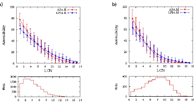
Relationship between residue accessibility and contact number. Accessibility
quantifies the exposure of residues to the solvent and this exposure is statistically related to the residue’s proximity to the protein surface. The residue contact number reflects its environment and obviously depends on accessibility. Samanta et al. noted an exponential relationship between residue contact number and accessible surface area (ASA) 78, 79. Samanta's protocol is different from ours in that two residues have as many contacts as atomic pairs in contact, whereas, in our case, amino acid i is in contact with amino acid j if at least one atomic pair is in contact. This enumeration of contacts is more similar to the coarse-grained method and is more straightforward.
Figure 2 displays variations of ASA (or LPIA) according to LCN for two typical and similarly sized residues: Lysine (K) and Methionine (M). However, K is more hydrophilic than M 2. Thus, K was found more often in the low LCN region reflecting characteristics of surface residues, whereas M had a higher propensity for larger LCN corresponding to the protein core (see distributions at the bottom of Figure 2). These profiles confirm some observations made by Samanta et al. The slope of the regression line is steeper for hydrophobic than for hydrophilic residues. The M profile reaches the asymptote at an LCN value of around 11 (Figure 2b), while K does not reach the asymptote before an LCN value of 16 (Figure 2a). As functions of LCN, two patterns were distinguished from the ASA and LPIA variations: (i) a decreasing linear relationship for low contact numbers, depending on residue hydrophobicity; (ii) an asymptote close to zero for high contact numbers. However, the LPIA curve was always below the ASA curve for low contact numbers, with the opposite relationship for high LCN values. For low LCN values, the dominance of ASA can be explained by the different normalization conventions: PIA is limited to 100% but ASA is not 54. For high LCN values, where accessibility is low, the difference is mainly due to the probe radius parameter used in NACCESS, 1.4 Å. As noted in ref 54, this value (close to the average van der Waals radius of water) is fairly large compared to surface sinuosities. Consequently, ASA often equaled 0 even when water-residue contacts occurred in the tessellation, meaning that LPIA was not equal to zero. LPIA is more sensitive than ASA in detecting small areas of
exposure to the solvent. Similar conclusions hold for the comparison of ASA with VPIA. The other contact methods led to similar observations; CCN and ACN showed similar curves with respect to variation in ASA. These trends were verified using other residues: the same analysis performed on Arginine (R) and Phenylalanine (F) gave similar results. Finally inter-residue contacts do not depend only on their volume, but also on their hydrophilicity and thus their accessibility.
Mean contact numbers deduced from distance-threshold and tessellation methods.
As discussed above, the usual approach for predicting contacts or defining Potentials of Mean Force is to set a distance threshold, . The literature contains a range of values for this parameter, depending on the data and scale (atom or residue) of interest. For contacts based on Cα, the cut-off distances used are typically 8, 10 or 12Å 69, 80, 81. If all the atoms in an amino acid are considered and if contacts are defined in terms of minimal atom-atom distances, threshold values are lower: = 4 Å 79, 82, 5.5 Å 83, and 4.5 Å 49. The advantage of the Laguerre or Voronoi tessellation methods is that they do not need any threshold parameter. Space filling defines the neighborhoods, and thus adapts to the local geometry of residue packing.
Table 1 gives the mean residue contact number calculated using the four contact methods (CCN, ACN, LCN and VCN). The overall mean CCN and ACN values were very similar (4.7-4.8), as were those for LCN and VCN (5.6-5.7). On average, the tessellation methods resulted in 0.8-0.9 more contacts per residue than the distance methods. The overall averages can be rendered equal by adjusting the threshold to nearly 5 Å for the all-atom method. But we kept the value 4.5 Å, more standard in the literature. Some specific mean CCN and ACN values showed large discrepancies, while this was not the case for LCN and VCN. For instance, ACN and CCN differed by 2.71 for tryptophan (W), 1.61 for tyrosine (Y) and 1.82 for phenylalanine (F), all defined as aromatic residues (see Table 1).
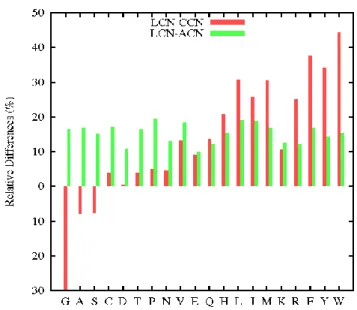
Figure 3 displays the relative differences between the tessellation method (LCN) and the distance-threshold methods (CCN or ACN). For small residues, LCN values are smaller than CCN, but larger for large residues; a fairly linear progression interpolates between these extremes. For small residues, the Cα method includes not only the nearest neighbors but also a few higher order ones, leading to a large overestimate. Similarly, the threshold approach misses some immediate neighbors for large residues, leading to a large underestimate. The effect of a fixed threshold value, independent of the residue size, can be clearly seen.
In addition, other particularities can be highlighted. M and K are two equally sized residues, but they showed strong discrepancies. More hydrophilic than M, K showed a small difference between LCN and CCN, whereas this difference was great for M. The same pattern can be observed for R and F. Thus, physico-chemical properties are also involved in determining contacts. K or R, are more often exposed and localized near the protein surface (mean ASA of K ~ 53% 54). Hence, their environment is less dense and only incompletely filled by neighboring residues. The direct consequence is a decrease in the mean contact number. Finally, this comparison revealed a relationship between mean contact number and the propensity to be at or close to the surface. This conclusion can be visualized in Figure 2.
At the finer, atomic scale, discrepancies between LCN and ACN did not depend on residue volumes (see Figure 3, green bars). Both methods take residue size into account through the number of atoms composing each residue. In this case, differences arose due to residue shape and physico-chemical properties. A group of small and/or hydrophobic residues (G, A, C, P, V, L, I, M) and some small polar residues (S and T) showed the greatest relative discrepancies, followed by the aromatic residues (H, F, Y, W), and finally by a group of polar or charged residues (D, N, E, Q, K, R). The discrepancies between LCN and ACN in the first two groups were comparable, whereas those of the third, polar-charged group were significantly smaller. Differences between LCN and ACN were always positive, indicating that some contacts found by the tessellation method cover a distance larger than 4.5 Å. Thus, the tessellation method (performed at atomic resolution) generally gives higher contact counts than the atomic threshold method and the observed discrepancies are partly correlated to residue hydrophobicity. As already mentioned, the global average difference can be reduced to zero by increasing the threshold to 5 Å; however the (dis)agreement was very poorly quantified by the PCC values. Indeed, the computations on a sample of thresholds ranging from 4.5 to 7.0 Å showed a constant PCC value close to 0.99, indicating that the mean LCN and ACN remained linearly related.
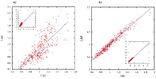
Analysis of global relative frequencies. The relative frequencies (rf) give information
on favored and unfavored contacts observed between residue pairs. Figure 4 shows the correlation of rf computed from Laguerre tessellation (LRF) with rf for the threshold approach at both scales, Cα (CRF) and all atoms (ARF). The frequency of Cysteine - Cysteine contacts was always high because of the special nature of disulfide bridges: CRF[C→C] = 6.45, ARF[C→C] = 5.00, VRF[C→C] = 6.50 and LRF[C→C] = 6.47. Therefore, the corresponding points were isolated and are only shown in an inset in Figure 4. The points in the (CRF, LRF) plot are scattered around the linear regression line and the correlation is indeed moderate
(PCC = 0.85, see Figure 4a), whereas a sharper linear correlation is observed between ARF and LRF (PCC = 0.98, see Figure 4b).
Laguerre and Voronoi tessellations gave highly similar results (see Supplementary data 2a). Overall, 207 pairs of amino acids (~50%) had the same LRF and VRF up to the third decimal. The greatest differences occurred for [C→C] and [Q→H], with values of -0.05 and 0.04, respectively. Hence, the subsequent analyses focused on Laguerre tessellation.
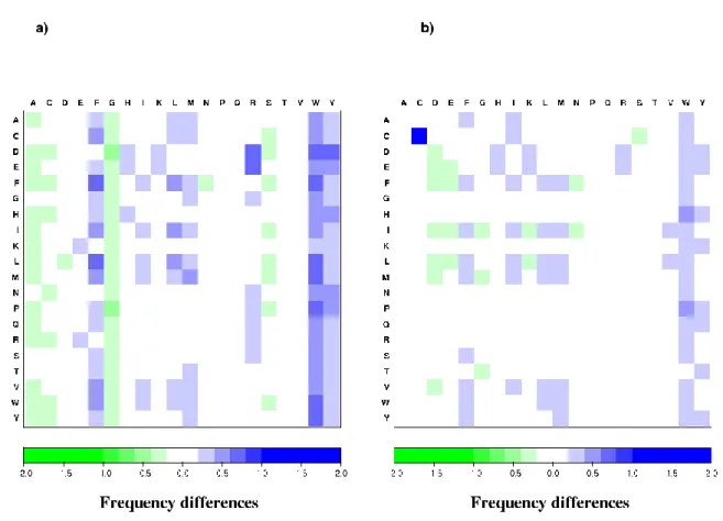
The details of the rf discrepancies are displayed as matrices in Figure 5, with a resolution threshold of 0.2 1. For any pair of amino acids, the contact tendency is simply the rf value compared to the value 1. Contacts tend to be either overrepresented, rf > 1, or underrepresented, rf < 1 (see also Supplementary data 2b). Three kinds of rf changes can be distinguished: (1) positive enhancement: relative contact frequency determined by the Laguerre tessellation (LRF) is significantly increased compared to the distance-threshold method, the trend does not change (overrepresented or underrepresented); (2) negative
enhancement: LRF is significantly decreased compared to the distance-threshold method,
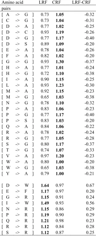
again without change in trends; (3) tendency inversion: over-represented contacts of one approach are found to be under-represented in another. The differences will be stated as variations of LRF with respect to ARF or CRF, considered as the reference. Among the 148 changes (37% of the matrix entries) found in the LRF-CRF matrix (see Figure 5a), 87 were positive enhancements (higher LRF values), 24 were negative enhancements and 37 were inversions (28 negative and 9 positive changes, representing nearly 10% of all the contacts.). Reductions (LRF lower) mainly occur with small residues (A, G, S). The contacts of aromatic residues (W, Y, F) and of some aliphatic/hydrophobic residues (M, L, I) were enhanced by LRF. These results corroborate those found for mean contacts (see above); the Cα distance method overestimated the contacts of small residues and, conversely, underestimated those of bulky residues, such as aromatic residues. As expected, the negative inversions (LRF < CRF) were observed mainly for contacts involving A and G residues (see Table 2). Interestingly, the positive inversions (LRF > CRF) were mainly observed for contacts involving Arginine (R): LRF-CRF = 0.64 for [D→R] and 0.64 for [E→R]. The enhanced LRF is well explained by the electronic attraction between the positively charged R and negatively charged D (or E); but the distances involved in those contacts are sometimes too large to be included in CRF.
Figure 5b displays the differences between LRFs and ARFs. Among the 84 changes (21% of all contacts), 65 are positive enhancements compared to 19 negative enhancements (lower LRF values). No inversions were observed. As expected, the LRF vs. ARF differences were weaker than those between LRF and CRF, both in number and amplitude. With the
exception of Cysteine - Cysteine contacts, which showed a difference of 1.47, the largest differences ranged from -0.24 to 0.49 for LRF vs. ARF against -0.40 to 0.78 for LRF vs. CRF. The positive changes mainly involved the contacts of aromatic residues, particularly W, but also Y, F, and aliphatic residues as L, M or I.
The contacts between Cysteines depart greatly from the other pairs of contacts. First, their relative frequency differences were LRF-CRF [C→C] = 0.02 and LRF-ARF [C→C] = 1.47. This result can be partly attributed to the fact that disulfide bonds can form between Cysteines, whose Cα distances range from 4.2 to 7.5 Å 84. The tessellation method is able to find contacts between two Cysteines separated by more than 4.5 Å. Thus, their contact numbers are equivalent to those found by the C method (with threshold of 8 Å), whereas the all-atom threshold at 4.5 Å fails to detect some of them.
The details of the relative frequencies reveal compensations in the contributions to the mean residue contact numbers. For instance for D, the relative difference LCN vs. CCN was 0.42 (see Figure 3) and is the sum of negative (A, C, G, S) and positive differences (H, K, R, W, Y) from Figure 5a. In other words, the mean contact counts sometimes even out sharper discrepancies revealed only when the contacts are sorted according to the species of both partners, as in relative frequencies.
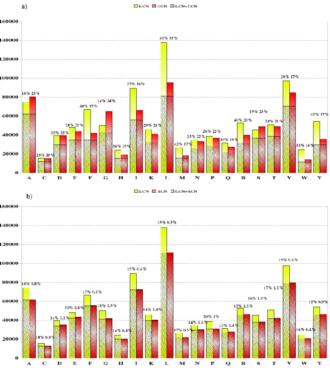
To obtain a more accurate view, contacts were sorted (see Figure 6) to determine which contacts were shared or different between methods. Three categories were distinguished: (1) contacts found in both the Laguerre and threshold methods, (2) contacts specific to the Laguerre tessellation method, (3) contacts specific to the distance-threshold method. In the bar graph given in Figure 6, the height of each bar represents the total contact count for the corresponding amino acid; the hatched section of the bar represents the contacts found by both methods. The non-hatched part of the bar corresponds to contacts found by only one of the two methods. In Figure 6a, of all the contacts found by the Cα threshold method, a proportion ranging from 16 to 34% depending on the amino acid, were only found by the C threshold method. The remainder, ranging from 66 to 84% of CCN, was observed for both (Cα and Laguerre) methods. Common contacts represented 47 to 84% of LCN, the contacts exclusively found for Laguerre tessellations, represented from 16 to 53 % of LCN.
Comparison of LCN with ACN (see Figure 6b) shows that the Laguerre-specific contacts ranged from 12 to 20%, compared to 0.4 to 3.2 % of ACN for the contacts specific to the all-atom distance method. These results demonstrate that both methods at the atomic scale (Laguerre tessellation and all-atom distance) share a larger set of common contacts than the
Laguerre tessellation with the Cα threshold method.
Analysis of relative frequencies according to protein size. The protein fold depends
on the length of the protein chain; protein size may therefore act on (un)favored contacts. We defined four classes of protein size (L being the number of residues in the protein chain):
L<150, 150 to 250, 251 to 400 and L>400 as proposed by Brocchieri et al. 85; and we examined the differences (dLRFs=LRFs-LRF), where LRFs is the Laguerre relative frequency calculated over the subset of proteins belonging to class s (size) whereas LRF is calculated over the entire databank (see Materials & Methods section).
To discern significant changes due to the contact method, we focused on the sets of amino acid pairs that satisfied the following criteria: (1) dLRF < 0.2 and dCRF (or dARF) > 0.2; (2) dLRF > 0.2 and dCRF (or dARF) < 0.2; (3) dLRF < -0.2 and dCRF (or dARF) > -0.2; (4) dLRF > -0.2 and dCRF (or dARF) < -0.2. Only the most striking changes are listed in Table 3; the selected amino acid pairs and the corresponding values of dLRF, dCRF and dARF are given for each protein size class.
Comparing dLRF and dCRF (or dARF), the greatest number of discrepancies was observed for small proteins (L<150). On average, small proteins had a larger conformational variety, with a smaller proportion of well-characterized secondary structures; therefore, more discrepancies may be expected in this class. For small proteins, dCRF differed from dLRF mainly for contacts involving bulky residues, such as Methionine (M) or Tryptophan (W), but also with hydrophobic residues, such as Cysteine (C), Glycine (G), Histidine (H), Isoleucine (I) and Valine (V). The greatest discrepancy was observed for [M→M], with a dLRF value of 0.46 compared to a dCRF valued of -0.05. Regarding dARF, the differences with dLRF were found for contacts with aromatic residues (F and W) and hydrophobic amino acids (C, G, H, I, S and T). The greatest discrepancy, observed for a dLRF value of -0.3 and a dARF value of 0.0, was for the [H→W] contact. Interestingly, for proteins including 150-250 amino acids, the selected changes involved contacts with only three main amino acid species (C, M and W), comparing dLRF with either dCRF or dARF. In the third protein size class (251-400), four amino acids were affected by changes in contact definition: C, H, I and M. Finally, in the last class, Cysteine (C) was involved in five of the seven recorded changes.
Globally, a linear relation was found between the drf's (such as dLRF and dCRF or with dARF, see Supplementary data 3). In order of increasing size, the (dLRF, dCRF) PCC for the four protein classes were 0.91, 0.82, 0.98, and 0.89, respectively. For (dLRF, dARF), the PCC were 0.91, 0.76, 0.95 and 0.88, respectively.
Analysis of rf according to distance along sequence. Among the possible types of
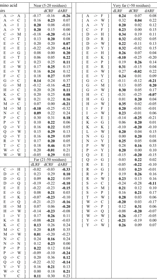
interactions, two major types may be distinguished: short- and long-rangeinteractions 86, 87. Long-range interactions are essential for the onset and prediction of protein folding 19, 40. To investigate the dependence on separation along the sequence, we defined three zones of distance along the protein sequence: near (5-20 residues), far (21-50 residues) and very far (>50 residues) as previously proposed 85. As above, a threshold of 0.2 (or -0.2) was chosen to characterize significant changes between dLRF and dCRF (or dARF). Table 4 summarizes those differences for all three contact methods. The comparison of dLRF with dCRF (or dARF) shows that the main discrepancies occurred at very far contacts. A simple hypothesis would relate this pattern to the fact that very far contacts preferentially involve β-sheets and some loops. We found small residues (C, G, P), some with charged (E, K), and aromatic residues (F, W and Y), were involved in the differences between methods. Among the large discrepancies, the following amino acid pairs were the most interesting ones: [D→W], [E→R], [W→W]. They all showed a dLRF value of > 0.2 whereas the dCRF value was < 0.1. Regarding dARF, the Laguerre contact excess dLRF mainly differed from dARF for contacts involving hydrophobic residues (F, H, M, Y and W) and Cysteine (C). The greatest discrepancy was for [W→W] pairs, with a dLRF value of 0.26 and a dARF value equal to -0.05.
For the other two distance zones, the selected partners were slightly different. For near contacts along the sequence, the discrepancies between dLRF and dCRF involved contacts with small, aromatic and hydrophobic residues (C, T, V, W and Y). The comparison of dLRF with dARF showed discrepancies for contacts mainly involving C, but also G, V, I. For the
far contacts, the set of residues involved in discrepancies was more heterogeneous, e.g., P, C,
W, Q, M and H for differences between dLRF and dARF; V, P, N, C, E, V, W, G, K for differences between dLRF and dCRF.
The analysis of rf as a function of distance along a sequence shows that the contacts or interactions between residues very distant along the sequence are difficult to determine and are more likely to result in discrepancies between the methods. As expected due to its size, its physico-chemical properties, and its implication in various interactions 82, W is often involved in the strongest discrepancies at any distance.
As in the previous section, the overall discrepancies can be summarized through correlation coefficients. For near contacts, the (dCRF, dLRF), the PCC value equaled 0.85 and 0.61 for dARF vs. dLRF. For far contacts, PCC values were 0.73 for dLRF vs. dCRF and 0.64 for dLRF vs. dARF, respectively. Finally, for very far contacts, the PCC was 0.57 for
dLRF vs. dCRF and 0.78 for dLRF vs. dARF. Therefore, the dLRF vs. dCRF relationship decreased with increasing contact distance, whereas the dLRF vs. dARF relationship increased. In some cases, because of its special position in Figure 4, the Cysteine - Cysteine interaction had a strong influence on the PCC values. For example, without taking [C→C] into account, PCC values for dCRF vs. dLRF were 0.73 (near), 0.73 (far) and 0.47 (very far). These values for dARF vs. dLRF were 0.44 (near), 0.59 (far) and 0.68 (very far). Except the
far contacts for dCRF, the absence of [C→C] decreased the PCC values. Finally, a difference
in contact distributions between secondary structures analyzed in each distance zone may also account for some PCC variations. For instance, Laguerre tessellation and the all-atom threshold method counted 26.4% and 28.0% of near contact frequency between two β-strands, respectively; whereas the Cα method resulted in 32.1%.
Analysis of rf according to secondary structures. The secondary structure elements
(SSEs) are local protein structures, known to be involved in the stability of protein 3D folds. The residue interactions and contacts observed in SSEs differ depending on their environment, thus a significant dependence on secondary structure may be expected. Indeed, α-helices are primarily maintained by short-range interactions, while β-sheets mainly involve long-range interactions. For specificity, the analysis was performed on the residues showing specific rf changes, i.e., important opposing changes in the two repetitive structures. As above, drf is the difference between the relative frequency calculated on a subset of residues (e.g., both i and j in α-helices) and its counterpart evaluated on the whole databank.
We only considered a limited number of representative cases. In Table 5, the amino acid pairs were selected as follows: helices) > 0.2 and drf (β-sheet) < -0.2} or {drf(α-helices) < -0.2 and drf (β-sheet) > 0.2} in at least one of the methods. In a majority of cases, the criterion was fulfilled by the Laguerre tessellation (dLRF). The values of the other methods (Cα and all-atom threshold methods) were often close, e.g., they had similar patterns. One exception was for [C→H] contacts in helices where the dLRF value was 0.01 while the dCRF value was -0.1 and the dARF, -0.21. Small residues, such as A or C, often appeared in the selected pairs. Cysteines are well known for maintaining protein structures by forming disulfide bridges, mainly in β-sheets.
As a general conclusion, discrepancies between the Laguerre tessellation and the distance-threshold methods (Cα method or all-atom) are modulated by both residue proximity along the sequence and their secondary structure.
tertiary or quaternary structure by forming relatively strong covalent bonds between Cysteines, which can be either quite distant in the amino acid sequence or even members of different peptide chains (quaternary case). However, the question of disulfide bridges is still a challenge 84, 88-92. A collection of criteria has been proposed to identify Cystine, based either on the distance between two sulfurs of less than 2.3 Å 3 or on the distance between Cysteine Cαs ranging from 4.2 to 7.5Å 84, 92. A Cystine is formed by the oxidation of two cysteine residues which covalently link and make a disulfide bond. A half-Cystine is a Cysteine involved in a disulfide bridge with another Cysteine to form a Cystine. In our analysis, Cystines were located using either a distance between two sulfurs lower than 2.1 Å, or the occurrence of a Laguerre (or Voronoi) face separating the sulfur polyhedra of two distinct Cysteines. The free Cysteines and half-Cystines were enumerated in each method and the results are given in Table 6. The contact criterion depended on the method. The threshold of 2.1 Å ensures that all the Cysteine (C) contacts found by the distance-threshold method form covalently bonded Cystines. All these contacts were also found by the tessellation methods. Indeed, covalent bonds imply that distances are short enough to be detected by all the considered methods. The tessellations included additional C-C contacts over distances greater than 2.1 Å still labeled as half-Cystines even if those bonds are almost certainly not covalent. Thus the number of half-Cystines detected by the Laguerre or Voronoi methods was higher than by the distance-threshold method (512 for the threshold method, 743 for Voronoi and 764 for Laguerre). Moreover, the odd number of half-Cystines produced using the Voronoi method indicates that some contacts involve more than two Cysteines. The C-C contact counts, detailed in Supplementary material 4, confirm that some proteins, such as the transferase (PDB code 1d0q 93) or the Vhs domain of Tom1 protein (PDB code 1elk 94), have three Cysteines that are in contact.
The tessellation methods do not account for either the physical nature of the interactions or the absolute distance, so there is no guarantee that the associated pairs of Cysteines are covalently bound. Nevertheless, these contacts reflect spatial closeness. More insight can be obtained from the correlation between (1) the distance between Cysteine sulfurs and (2) the area of the corresponding face in Laguerre tessellation, displayed in Figure 7. The data were split into two distinct clusters, clearly separated along the distance spectrum: one sharply centered on a mean distance of 2 Å, certainly involving the covalently bound Cystines, and the other, scattered at values greater than 3.2 Å, corresponding to non-covalent contacts. The gap between 2.1 and 3.2 Å leaves no ambiguity in qualifying these contacts. While the covalent distance is fixed to nearly 2 Å, the corresponding face area spreads over
quite a broad interval ranging from 8 to 13 Ų. For distances greater than 3 Å, the distance and area showed a negative correlation and a middle range PCC value of -0.72, similar to normal kinds of contacts.
Figure 8 represents the molecular configurations of the four main cases observed: covalent distance (< 2.1 Å) and a bottom range area (see Figure 8a), covalent distance and top range area (see Figure 8b), normal distance (> 3 Å) and small area (see Figure 8c), normal distance and larger area (see Figure 8d). Figures 8c and 8d demonstrate the importance of the orientation of the Cysteines on the Laguerre face area. When both Cysteines are parallel, the contact tends to be small, with a small face area (see Figure 8c), while the area increases when the Cysteine sulfurs face each other as in Figure 8d.
In summary, the distance method is very effective in selecting only the covalently linked Cystines, while the tessellation method, not limited by any threshold, detects the relative proximity of sulfurs even in absence of any tight bond interaction. Moreover, distance is not the only factor; the conformation around the Cysteines also plays a role in the contacts found by tessellation methods. Therefore, tessellations, especially the Laguerre tessellation with well-tuned weights, may even provide deeper insight into the geometry of the contacts.
C
ONCLUSIONCurrently, the knowledge of protein folding still poses a challenge for fully understanding the functionality of proteins and predicting their structure. Exploring the interactions and contacts between residues is a key step to furthering our knowledge in this area. Here, we proposed a detailed analysis of the contacts which can be specified by geometrical criteria, whereas interactions rely on forces or energies. We carried out a comparative analysis of two contact definitions: distance-threshold methods and tessellation methods. The distance-threshold method is useful and realistic when the contacts surrounding a residue are specified by a particular distance range. This type of method does not need any solvent around the protein, which may save computer memory and run time. The tessellation method provides a more realistic representation of the local ordering in the structure; the contacts deduced from tessellation essentially consist of a complete list of neighbors in the first layer around any residue. The method is flexible and adapts itself to density inhomogeneities. However, this tessellation approach needs the presence of solvent if accessible residues are to be incorporated in the analysis. The Voronoi tessellation method does not depend on any parameter, but it is known to even out local inhomogeneities, which
may lead to some undesirable bias 54. At the coarse-grained and atomic scales, the Laguerre (or weighted Voronoi) tessellation method provides the most precise account of space occupation by the constituent atoms, residues or molecular units. However, it relies on a set of weights that need tuning 51, 54, even though the simple formula w = r2, in terms of the Van der Waals radius r, was found to be optimal at the atomic scale. Regarding contacts, Laguerre and Voronoi partitions give very similar results, with about 99% of common contacts (see Supplementary data 5). The few cases of discrepancies mainly involve residues at the protein surface.
Much more significant are the discrepancies found in comparing the tessellation and distance-threshold methods. On average, these differences compensate each other, an indication that the threshold has been set to an appropriate intermediate value. However, the discrepancies become more and more visible when the contacts are differentiated by amino acid species, or even by pairs of species as in the relative frequencies.
Acknowledgements. A PhD grant to Dr. Esque Jérémy. from the French Ministry of Higher Education and Research is acknowledged. We thank Xabier Oyharçabal for his contribution to the early development of VLDP and all the developers of the freely available software which greatly facilitated our work (cited in Materials & Methods section). This work was supported by grants from the French Ministry of Research, Paris Diderot University Paris 7, French National Center for Scientific Research (CNRS), French National Institute for Blood Transfusion (INTS) and French National Institute for Health and Medical Research (INSERM).
Supporting Information Available. Supplementary data are available on 1. PCC values for the correlation between residue volumes and mean contacts, 2. Relative frequencies from tessellations; differences between Laguerre and Voronoi data (2a) and Laguerre LRF values (2b), 3. (dLR, dCRF) correlations vs. protein size. 4. A list of proteins is also provided including Cysteine-Cysteine contact counts. 5. Finally, the contacts shared by the Laguerre and Voronoi methods are displayed in the same way as Fig. 6. This material is available free of charge via the Internet at http://pubs.acs.org/.
Figure Captions
Figure 1. Plot of mean residue contact number (LCN) against mean Laguerre volume (Å3).
Mean values are taken over all residues (a), restricted to buried residues (ASA = PIA = 0) (b), or restricted to exposed residues (ASA > 25%) (c). Similar plots were obtained for Voronoi tessellations (not shown). Linear least-squares regression lines are indicated (dashed lines): (a) y = 0.03 Å-3 x + 1.13; (b) y = 0.05 Å-3 x + 3.94; (c) y = 0.03 Å-3 x + 1.97.
Figure 2. Mean accessible surface area (ASA) and mean Laguerre polyhedral interface area (LPIA) with respect to the Laguerre contact number (LCN). Two typical residues are
illustrated: a) Lysine and b) Methionine . The lines are fits to the following function: y = a(1-erf(bx)). Lower panels for both species give the residue population with respect to LCN to show its influence on variation in accessibility.
Figure 3. Discrepancies in relative mean contact number between the Laguerre and distance methods. The bar heights indicate the percent of relative differences (LCN – ACN) / LCN or
Figure 4. Correlation between relative frequencies given by tessellation and distance-threshold methods. LRF is plotted against a) CRF and b) ARF. The lines correspond to
least-square fit: a) f(x) = 1.4 x - 0.3, b) f(x) = 1.6 x - 0.6. The insets show the complete data including the isolated Cysteine-Cysteine pair.
Figure 5. Discrepancies in relative frequency between the tessellation and distance-threshold methods. The rf differences are given as matrices indexed by the amino acid species (a)
Figure 6. Contacts found in the Laguerre and distance-threshold methods. The total contact numbers of each amino acid species, computed over the whole databank, are displayed as bar graphs for a) the Laguerre vs. Cα distance methods, b) the Laguerre vs. all-atom distance methods. The hatched portion of the bars represents the contacts common to both methods. Conversely, for each residue, the remaining percentages give the proportion of contacts found exclusively by each method (solid-colored bars without hatching).
Figure 7. Laguerre face area vs. bond distance in tessellation for contacts between Cysteine sulfurs. Each point represents a Laguerre contact between the S atoms of two Cysteines.
Figure 8. Four typical configurations of Cysteine pairs in contact. The Cysteines are shown as balls. The blue polygon of area A, is the Laguerre face between the Cysteine sulfurs, distance d apart. a) 1lpb 95, d=2.04 Å, A=7.71 Å2; b) 1pl3 96, d=2.04 Å, A=12.80 Å2; c) 2bm5 97, d=5.025 Å, A=0.09 Å2; d) 1b25 98, d= 5.57 Å, A=7.35 Å2. Views made with PyMol.
Table1. Mean residue contact number calculated using a panel of four contact methods. The mean residue contact numbers and the corresponding standard deviations σ were computed for the distance-threshold methods (CCN, ACN) and the tessellation methods (VCN, LCN).
N, residue count; N, total residue count in the databank; avg(CN), global weighted average
mean residue contact numbers.
AA N CCN σ ACN σ VCN σ LCN σ A 15160 5.3 3.0 4.1 2.2 4.9 2.6 4.9 2.6 C 2266 6.6 2.8 5.7 2.1 6.8 2.5 6.9 2.5 D 11123 3.5 2.7 3.2 2.3 3.5 2.6 3.6 2.6 E 13189 3.3 2.4 3.3 2.3 3.6 2.6 3.7 2.6 F 7626 5.5 2.6 7.3 2.8 8.7 3.4 8.8 3.4 G 13336 4.9 3.3 3.1 2.0 3.7 2.4 3.8 2.4 H 4212 4.6 2.8 4.9 2.8 5.7 3.2 5.8 3.2 I 11087 6.0 2.7 6.6 2.5 8.0 3.0 8.1 3.0 K 11252 3.7 2.4 3.6 2.3 4.0 2.6 4.1 2.7 L 17818 5.4 2.6 6.3 2.5 7.7 3.1 7.7 3.1 M 3449 5.4 2.7 6.4 2.8 7.6 3.4 7.7 3.4 N 8135 4.1 2.8 3.7 2.5 4.2 2.9 4.2 2.9 P 8596 4.3 2.9 3.6 2.4 4.4 2.9 4.5 2.9 Q 7035 3.9 2.6 3.9 2.5 4.4 2.9 4.5 2.9 R 9382 4.2 2.6 4.9 2.9 5.6 3.3 5.6 3.3 S 10869 4.5 3.0 3.5 2.3 4.1 2.7 4.2 2.7 T 10044 4.9 2.9 4.2 2.4 5.0 2.9 5.1 2.9 V 13601 6.2 2.8 5.8 2.4 7.1 2.9 7.2 2.9 W 2605 5.3 2.5 8.0 3.0 9.3 3.5 9.4 3.5 Y 6648 5.4 2.7 7.0 3.0 8.1 3.5 8.2 3.5 ∑ N 187433 avg(CN) 4.8 4.7 5.5 5.6
Table 2. Inversion cases in the comparison of LRF with CRF for the whole databank. Boldface indicates the largest values (LRF or CRF) in the comparison.
Amino acid LRF CRF LRF-CRF pairs [ A -> G ] 0.73 1.05 -0.32 [ C -> G ] 0.73 1.04 -0.31 [ D -> A ] 0.77 1.02 -0.25 [ D -> C ] 0.93 1.19 -0.26 [ D -> G ] 0.77 1.17 -0.40 [ D -> S ] 0.89 1.09 -0.20 [ E -> A ] 0.78 1.04 -0.26 [ F -> A ] 0.82 1.02 -0.20 [ G -> G ] 0.93 1.30 -0.37 [ H -> A ] 0.77 1.01 -0.24 [ H -> G ] 0.72 1.10 -0.38 [ I -> A ] 0.90 1.15 -0.25 [ L -> A ] 0.93 1.23 -0.30 [ M -> A ] 0.92 1.15 -0.23 [ M -> G ] 0.65 1.03 -0.38 [ N -> G ] 0.78 1.10 -0.32 [ P -> A ] 0.83 1.06 -0.23 [ P -> G ] 0.77 1.17 -0.40 [ P -> S ] 0.83 1.03 -0.20 [ Q -> A ] 0.84 1.06 -0.22 [ R -> A ] 0.78 1.02 -0.24 [ R -> G ] 0.77 1.05 -0.28 [ S -> G ] 0.80 1.17 -0.37 [ T -> G ] 0.74 1.07 -0.33 [ V -> A ] 0.97 1.20 -0.23 [ W -> A ] 0.80 1.00 -0.20 [ W -> G ] 0.65 1.03 -0.38 [ Y -> A ] 0.79 1.00 -0.21 [ D -> W ] 1.64 0.97 0.67 [ E -> F ] 1.17 0.97 0.20 [ G -> R ] 1.15 0.91 0.24 [ I -> W ] 1.49 0.93 0.56 [ N -> R ] 1.15 0.86 0.29 [ P -> R ] 1.19 0.90 0.29 [ Q -> R ] 1.21 0.98 0.23 [ R -> R ] 1.12 0.84 0.28 [ S -> R ] 1.12 0.87 0.25
Table 3. Influence of protein size on relative frequencies. Four classes of protein size are considered: <150, 150-250, 251-400, >400 (residue number). dLRF = LRFs – LRF is the difference between the average restricted to proteins of the specified size and the global average, computed using the Laguerre method. dCRF and dARF are defined analogously for the distance methods. The listed amino acid pairs were selected according to one of the criteria (1), (2), (3) or (4) in Analysis of relative frequencies according to protein size section.
Amino acid <150 150-250 pairs dCRF dARF dLRF dCRF dARF
[ C -> H ] -0.22 -0.10 -0.27 [ C -> W ] -0.16 -0.23 -0.51 [ C -> I ] -0.27 -0.26 -0.12 [ H -> C ] 0.17 0.24 0.14 [ C -> P ] 0.05 0.07 0.22 [ K -> W ] 0.20 0.12 0.13 [ C -> V ] -0.23 -0.19 -0.20 [ M -> C ] 0.04 0.21 -0.13 [ D -> G ] -0.10 -0.21 -0.07 [ M -> M ] -0.02 -0.18 -0.25 [ D -> H ] -0.27 -0.10 -0.26 [ W -> C ] -0.09 -0.26 -0.24 [ F -> C ] 0.22 0.31 0.11 [ W -> W ] 0.14 0.18 0.27 [ F -> F ] 0.29 0.21 0.16 [ G -> G ] -0.25 -0.37 -0.19 251-400 [ H -> K ] 0.10 0.13 0.29 dLRF dCRF dARF [ H -> T ] -0.20 -0.22 -0.09 [ C -> H ] 0.15 0.09 0.20 [ H -> W ] 0.30 0.24 0.00 [ C -> I ] 0.21 0.21 0.16 [ K -> C ] 0.20 0.18 0.12 [ H -> C ] 0.14 0.08 0.22 [ M -> F ] 0.12 0.16 0.31 [ I -> C ] 0.18 0.20 0.15 [ M -> I ] 0.06 0.24 -0.01 [ M -> M ] 0.11 0.30 0.19 [ M -> M ] 0.46 -0.05 0.25 [ M -> W ] -0.20 0.12 0.06 [ N -> S ] -0.19 -0.21 -0.01 [ Q -> C ] 0.13 0.09 0.29 [ R -> W ] -0.16 -0.04 -0.21 [ S -> C ] 0.38 0.41 0.19 >400 [ S -> H ] -0.17 -0.21 -0.20 dLRF dCRF dARF [ S -> N ] -0.23 -0.20 -0.02 [ C -> M ] 0.28 0.09 0.22 [ T -> C ] 0.14 0.22 0.19 [ C -> R ] 0.20 0.19 0.20 [ T -> H ] -0.28 -0.23 -0.15 [ H -> S ] 0.09 0.20 0.03 [ W -> M ] -0.24 -0.01 -0.19 [ M -> C ] 0.14 0.00 0.25 [ W -> T ] -0.10 -0.22 0.01 [ Q -> C ] -0.11 -0.21 -0.07 [ W -> W ] -0.24 -0.08 -0.36 [ S -> C ] -0.21 -0.16 -0.12 [ Y -> I ] 0.16 0.09 0.20 [ Y -> W ] -0.17 -0.11 -0.25
Table 4. Relative frequency modulation according to distance along the sequence. Excess dLRF, dCRF and
dARF induced by specifying the distance between residue are compared for three distance zones: near (5-20 residues), far (21-50 residues), very far (>50 residues). Only the cases with one absolute value >0.2 are presented.
Amino acid Near (5-20 residues) Very far (>50 residues)
pairs dCRF dARF dLRF dCRF dARF [ A -> A ] -0.17 -0.16 -0.26 [ A -> F ] 0.24 0.07 0.08 [ A -> C ] 0.16 0.23 0.07 [ A -> W ] 0.32 0.04 0.22 [ A -> I ] 0.20 0.08 -0.01 [ A -> Y ] 0.20 0.02 0.12 [ A -> V ] 0.20 0.15 0.00 [ C -> F ] 0.23 0.00 0.15 [ C -> M ] -0.18 -0.20 -0.14 [ D -> H ] 0.34 0.19 0.11 [ C -> T ] 0.13 0.20 0.08 [ D -> R ] 0.32 -0.02 0.05 [ E -> C ] 0.20 0.20 0.07 [ D -> W ] 0.22 -0.11 0.13 [ E -> E ] -0.22 -0.20 -0.14 [ D -> Y ] 0.32 -0.02 0.15 [ E -> G ] 0.08 0.00 0.20 [ E -> H ] 0.26 0.07 0.04 [ E -> T ] 0.06 0.05 0.22 [ E -> K ] -0.10 -0.25 -0.20 [ E -> V ] 0.23 0.25 0.11 [ E -> P ] 0.19 0.26 0.14 [ E -> W ] 0.17 0.25 0.15 [ E -> R ] 0.31 -0.15 0.04 [ E -> Y ] 0.16 0.24 0.12 [ E -> W ] 0.27 -0.02 0.22 [ F -> C ] 0.18 0.27 0.09 [ E -> Y ] 0.24 0.01 0.09 [ G -> C ] 0.14 0.24 0.37 [ G -> C ] -0.11 -0.12 -0.21 [ G -> M ] -0.12 -0.16 -0.22 [ G -> M ] 0.13 0.05 0.20 [ H -> C ] 0.20 0.28 0.11 [ G -> W ] 0.30 0.05 0.17 [ K -> C ] 0.20 0.25 0.08 [ H -> C ] -0.31 -0.25 -0.07 [ K -> W ] 0.21 0.22 0.16 [ H -> G ] 0.01 0.20 0.04 [ M -> C ] 0.07 0.00 -0.21 [ H -> W ] 0.35 0.02 -0.05 [ M -> M ] -0.10 -0.25 -0.32 [ I -> F ] 0.20 -0.01 -0.01 [ N -> C ] 0.09 0.22 0.24 [ I -> W ] 0.23 -0.01 0.06 [ P -> C ] 0.30 0.31 0.18 [ K -> E ] -0.14 -0.25 -0.21 [ P -> Y ] 0.10 0.22 0.06 [ K -> G ] 0.06 0.20 0.01 [ Q -> V ] 0.16 0.22 0.05 [ K -> K ] -0.10 -0.20 -0.10 [ Q -> W ] 0.15 0.29 0.13 [ L -> W ] 0.20 0.04 0.15 [ Q -> Y ] 0.16 0.29 0.09 [ N -> G ] 0.00 0.20 0.01 [ R -> V ] 0.17 0.20 0.05 [ N -> Y ] 0.25 0.05 0.08 [ T -> C ] 0.18 0.46 0.19 [ P -> W ] 0.28 0.16 0.33 [ W -> C ] 0.20 -0.01 0.21 [ P -> Y ] 0.20 0.00 0.10 [ W -> W ] -0.05 0.29 0.01 [ Q -> E ] -0.15 -0.20 -0.15 Far (21-50 residues) [ Q -> G ] 0.03 0.22 0.02 dLRF dCRF dARF [ R -> E ] -0.05 -0.22 -0.10 [ C -> H ] -0.02 -0.03 -0.33 [ R -> G ] 0.03 0.23 -0.01 [ D -> C ] 0.23 0.29 0.10 [ R -> P ] 0.19 0.26 0.16 [ D -> G ] 0.09 0.22 0.09 [ R -> W ] 0.23 0.13 0.16 [ D -> Q ] -0.19 -0.22 -0.10 [ S -> C ] -0.24 -0.28 -0.11 [ E -> E ] -0.22 -0.23 -0.15 [ S -> M ] 0.21 0.12 0.10 [ E -> G ] 0.08 0.21 0.03 [ S -> P ] 0.16 0.21 0.17 [ E -> K ] -0.07 -0.23 -0.10 [ T -> W ] 0.28 0.03 0.06 [ E -> Q ] -0.21 -0.23 -0.16 [ W -> C ] -0.20 0.03 -0.17 [ H -> M ] 0.07 0.06 -0.20 [ W -> P ] 0.12 0.31 0.06 [ H -> W ] -0.14 -0.23 -0.08 [ W -> Q ] -0.08 -0.20 -0.07 [ I -> V ] 0.17 0.26 0.11 [ W -> W ] 0.26 -0.17 -0.05 [ K -> E ] -0.08 -0.21 -0.03 [ Y -> C ] -0.21 -0.19 0.00 [ K -> C ] 0.13 0.26 0.24 [ Y -> W ] 0.26 0.09 0.07 [ M -> C ] 0.20 0.15 0.35 [ M -> W ] 0.01 -0.20 -0.23 [ N -> C ] 0.24 0.16 0.24 [ N -> N ] 0.12 0.23 0.00 [ P -> P ] 0.22 0.12 0.04 [ P -> W ] -0.09 -0.10 -0.24 [ Q -> C ] 0.20 0.36 0.12 [ Q -> Q ] -0.22 -0.32 -0.14 [ V -> V ] 0.16 0.21 0.13 [ W -> C ] 0.00 0.18 0.21 [ Y C ] 0.11 0.30 0.23
Table 5. Contact differences for α-helices and β-sheets. The table gives the relative frequency changes (drf) due to the secondary structure environment of the residues. Only the amino acid pairs showing contrasting changes are displayed, i.e., both (helix and sheet) drf of absolute value > 0.2 but of opposite sign, in at least one of the methods. The pairs satisfying this criterion are displayed in bold.
Amino acid dLRF dCRF dARF pairs sheet helix sheet helix sheet
[ H -> E ] -0.23 0.33 -0.17 0.29 -0.18 0.19 [ I -> A ] -0.22 0.21 -0.16 0.17 -0.13 0.14 [ L -> A ] -0.22 0.24 -0.21 0.19 -0.16 0.14 [ P -> M ] -0.11 0.18 -0.06 0.1 -0.24 0.26 [ T -> Q ] -0.22 0.23 -0.15 0.19 -0.15 0.22 [ V -> A ] -0.2 0.28 -0.17 0.26 -0.1 0.21 [ W -> Q ] -0.25 0.25 -0.24 0.22 -0.21 0.33 [ C -> F ] 0.38 -0.42 0.2 -0.44 0.18 -0.31 [ C -> H ] -0.01 -0.12 0.1 -0.04 0.21 -0.2 [ C -> V ] 0.24 -0.46 0.2 -0.44 0.13 -0.35 [ F -> F ] 0.21 -0.62 0.03 -0.35 0.06 -0.44 [ I -> C ] 0.1 -0.25 0.2 -0.3 0.01 -0.18 [ L -> C ] 0.16 -0.17 0.2 -0.21 0.06 -0.1 [ M -> C ] 0.26 -0.29 0.31 -0.21 0.01 -0.15 [ M -> F ] 0.2 -0.51 0.13 -0.34 0.09 -0.39 [ M -> V ] 0.22 -0.49 0.14 -0.45 0.15 -0.38 [ W -> F ] 0.22 -0.57 0.04 -0.29 0.04 -0.35
Table 6. Counts of Cysteine-Cysteine contacts and disulfide bridges. The numbers of free cysteines (Cysh) (no S-S contact with other Cysteine) and of half-Cystines (Cyss) are indicated as provided by the three contact methods. “Threshold” stands for the all-atom threshold method. The half-Cystines are defined either by a distance shorter than 2.1 Å in the threshold method or, in the tessellation method, by a face shared by two sulfurs (in this case, the contact may be covalent or not).
Threshold Voronoi Laguerre Cysh 1754 1523 1502 Cyss 512 743 764