The Lorentz force effect on the On-Off dynamo intermittency

HAL Id: hal-00175646

https://hal.archives-ouvertes.fr/hal-00175646

Preprint submitted on 28 Sep 2007

HAL is a multi-disciplinary open access

archive for the deposit and dissemination of

sci-entific research documents, whether they are

pub-lished or not. The documents may come from

teaching and research institutions in France or

abroad, or from public or private research centers.

L’archive ouverte pluridisciplinaire HAL, est

destinée au dépôt et à la diffusion de documents

scientifiques de niveau recherche, publiés ou non,

émanant des établissements d’enseignement et de

recherche français ou étrangers, des laboratoires

publics ou privés.

The Lorentz force effect on the On-Off dynamo

intermittency

Alexandros Alexakis, Yannick Ponty

To cite this version:

Alexandros Alexakis, Yannick Ponty. The Lorentz force effect on the On-Off dynamo intermittency.

2007. �hal-00175646�

hal-00175646, version 1 - 28 Sep 2007

Alexandros Alexakis, Yannick Ponty

Laboratoire Cassiop´ee, Observatoire de la Cˆote d’Azur, BP 4229, Nice Cedex 04, France

An investigation of the dynamo instability close to the threshold produced by an ABC forced flow is presented. We focus on the on-off intermittency behavior of the dynamo and the counter-effect of the Lorentz force in the non-linear stage of the dynamo. The Lorentz force drastically alters the statistics of the turbulent fluctuations of the flow and reduces their amplitude. As a result much longer burst (on-phases) are observed than what is expected based on the amplitude of the fluctuations in the kinematic regime of the dynamo. For large Reynolds numbers, the duration time of the “On” phase follows a power law distribution, while for smaller Reynolds numbers the Lorentz force completely kills the noise and the system transits from a chaotic state into a “laminar” time periodic flow. The behavior of the On-Off intermittency as the Reynolds number is increased is also examined. The connections with dynamo experiments and theoretical modeling are discussed.

PACS numbers: 47.65.-d,47.20.Ky,47.27.Sd,52.65.Kj

I. INTRODUCTION

Dynamo action, the self amplification of magnetic field due to the stretching of magnetic field lines by a flow, is considered to be the main mechanism for the generation of magnetic fields in the universe [1]. To that respect many experimental groups have successfully attempted to reproduce dynamos in liquid sodium laboratory ex-periments [2, 3, 4, 5, 6, 7, 8]. The induction exex-periments [9, 10, 11, 12, 13, 14, 15, 16, 17, 18] studying the response of an applied magnetic field inside a turbulent metal liq-uid represent also a challenging science. With or without dynamo instability the flow of a conducting fluid forms complex system, with a large degree of freedoms and a wide branch of non linear behaviors.

In this work we focus on one special behavior: the On-Off intermittency or blowout bifurcation [19, 20]. On-off intermittency is present in chaotic dynamical systems for which there is an unstable invariant manifold in the phase space such that the unstable solutions have a growth rate that varies strongly in time taking both positive and neg-ative values. If the averaged growth rate is sufficiently smaller than the fluctuations of the instantaneous growth rate, then the solution can exhibit on-off intermittency where bursts of the amplitude of the distance from the invariant manifold are observed (when the growth rate is positive) followed by a decrease of the amplitude (when the growth rate is negative). (See [21, 22] for a more precise definition).

On-Off intermittency has been observed in different physical experiments including electronic devices, elec-trohydrodynamic convection in nematics, gas discharge plasmas, and spin-wave instabilities [23]. In the MHD context, near the dynamo instability onset, the On-Off intermittency has been investigated by modeling of the Bullard dynamo [24]. Using direct numerical simulation [21, 22] were able to observe On-Off intermittency solving the full MHD equations for the ABC dynamo, (here we present an extended work of this particular case). On-Off intermittency has also been found recently for a

Taylor-Green flow [25]. Finally, recent liquid metal experimental results (VKS) [26] show some intermittent behavior, with features reminiscent of on-off self-generation that moti-vated our study.

For the MHD system we are investigating the evolu-tion of the magnetic energy Eb =

1

2R b

2

dx3

is given by ∂tEb = R b(·b∇)u − η(∇b)2dx3. If the velocity field

has a chaotic behavior in time the right hand side of the equation above can take positive or negative val-ues and can be modeled as multiplicative noise. A sim-ple and proved very useful way to model the behav-ior of the magnetic field during the on-off intermittency is using a stochastic differential equation (SDE-model) [19, 20, 27, 28, 29, 30, 31, 32, 33, 34, 35]:

∂tEb= (a + ξ)Eb− N L(Eb) (1)

where Eb is the magnetic energy, a is the long time

av-eraged growth rate, ξ models the noise term typically assumed to be white (see however [34, 35]) and of am-plitude D such that hξ(t)ξ(t′

)i = 2Dδ(t − t′

). N L is a non-linear term that guaranties the saturation of the magnetic energy to finite values typically taken to be N L(X) = X3

for investigations of supercritical bifurca-tions or N L(X) = X5

− X3

for investigations of subcrit-ical bifurcations. Alternative, an upper no-flux bound-ary is imposed at Eb = 1. In all these cases

(indepen-dent of the non-linear saturation mechanism) the above SDE leads to the stationery distribution function that for 0 < a < D has a singular behavior at Eb = 0:

P (Eb) ∼ E_ba/D−1 indicating that the systems spends a

lot of time in the neighborhood of Eb= 0. This is

singu-larity is the signature of On-Off intermittency. Among other predictions of the SDE model here we note that the distribution of the duration time of the “off” phases fol-lows a power law behavior P DF (∆Tof f) ∼ ∆T

−1_.5

of f , all

moments of the magnetic energy follow a linear scaling with a, hEm

b i ∼ a, and for a = 0 the set of the burst has

2

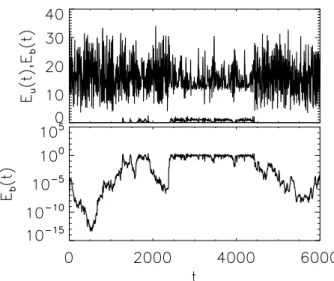
FIG. 1: A typical example of a burst. The top panel shows the evolution of the kinetic energy (top line) and magnetic energy (bottom line). The bottom panel shows the evolution of the magnetic energy in a log-linear plot. During the on phase of the dynamo the amplitude of the noise of the kinetic energy fluctuations is significantly reduced. The runs were for the parameters Gr = 39.06 and GM = 50.40.

In this dynamical system eq.(1) however the noise am-plitude or the noise proprieties do not depend on the amplitude of the magnetic energy. However, in the MHD system, when the non-linear regime is reached, the Lorentz force has a clear effect on the the flow such as the decrease of the small scale fluctuation, and the decrease of the local Lyapunov exponent [36, 37]. Some cases, the flow is altered so strongly that the MHD dynamo system jumps into an other attractor, that cannot not sustain any more the dynamo instability [38]. Although the ex-act mechanism of the saturation of the MHD dynamo is still an open question that might not have a universal answer, it is clear that both the large scales and the tur-bulent fluctuations are altered in the non-linear regime and need to be taken into account in a model.

Figure 1 demonstrates this point, by showing the evo-lution of the kinetic and magnetic energy as the dynamo goes through On- and Off- phases. During the On phases although the magnetic field energy is an order of magni-tude smaller than the kinetic energy both the mean value and the amplitude of the observed fluctuations of the ki-netic energy are significantly reduced. As a result the On-phases last a lot longer than what the SDE-model would predict. With our numerical simulations, we aim to describe which of the On-Off intermittency proprieties are affected through the Lorentz force feed-back.

This paper is structured as follows. In the next section II we discuss the numerical method used. In section III A we present the table of our numerical runs and discuss the dynamo onset. Results for small Reynolds numbers investigating the transition from a laminar dynamo to on-off intermittency are presented in III B, and the results on fully developed on-off intermittency behavior are given in

section III C. Conclusions, and implications on modeling and on the laboratory experiments are given in the last section IV.

II. NUMERICAL METHOD

Our investigation is based on the numerical integration of the classical incompressible MagnetoHydroDynamic equations (MHD) (2) in a full three dimensional peri-odic box of size 2π, with a parallel pseudo-spectral code. The MHD equations are:

∂tu+ u · ∇u = −∇P + (∇ × b) × b + ν∇2u+ f

∂tb = ∇ × (u × b) · u + η∇ 2

b ₍₂₎ along with the divergence free constrains ∇ · u = ∇ · b = 0. Where u is the velocity, b is the magnetic field (in units of Alfv´en velocity), ν the molecular viscosity and η the magnetic diffusivity. f is an externally applied force that in the current investigation is chosen to be the ABC forcing [39] explicitly given by

f _{= ˆx(A sin(kzz) + C cos(kyy))} ˆ

y(B sin(kxx) + A cos(kzz)) (3)

ˆ

z(C sin(kyy) + B cos(kxx))

with all the free parameters chosen to be unity A = B = C = kx= ky = kz= 1.

The MHD equations have two independent control pa-rameters that are generally chosen to be the kinetic and magnetic Reynolds numbers defined by: Re = U L/ν and RM = U L/η respectably, where U is chosen to

be the root mean square of the velocity (defined by U = p2Eu/3, where Eu is the total kinetic energy

of the velocity) and L is the typical large scale here taken L = 1.0. Alternatively we can use the ampli-tude of the forcing to parametrize our system in which case we obtain the kinetic and magnetic Grashof numbers Gr = F L3

/ν2

and GM = F L3/νη respectably. Here F

is the amplitude of the force that is taken to be unity F =p(A2_{+ B}2_{+ C}2_{)/3 = 1 following the notation of}

[53].

We note that in the laminar limit the two different sets of control parameters are identical Gr = Re and GM = RM but in the turbulent regime the scaling

Gr ∼ Re2

and GM ∼ ReRM is expected. In the

ex-amined parameter range the velocity field fluctuates in time generating uncertainties in the estimation of the root mean square of the velocity and then the Reynolds numbers. For this reason in this work we are going to use the Grashof numbers as the control parameters of our system.

Starting with a statistically saturated velocity, we in-vestigate the behavior of the kinetic and magnetic en-ergy in time by introducing a small magnetic seed at t = 0 and letting the system evolve. When the mag-netic Grashof (Reynolds) number is sufficiently large the

magnetic energy grows exponentially in time reaching the dynamo instability. We have computed the dynamo on-set for different kinematic Grashof (Reynolds) numbers (III.A) starting from small Gr = 11.11 that the flow ex-hibits laminar ABC behavior to larger values of Gr (up to Gr = 625.0) that the flow is relatively turbulent.

Typical duration of the runs were 105

turn over times although in some cases even much longer inte-gration time was used. For each run during the kine-matic stage of the dynamo the finite time growth rate aτ(t) = τ−1log(Eb(t + τ )/Eb(t) was measured. The

long time averaged growth rate was then determined as a = limτ →∞aτ(0) and the amplitude of the noise D

was the measured based on D = τ h(a − aτ)2i/2 (see

[21, 22]). Typical value of τ was 100 while the for long time average the typical averaging time ranged from 104

to 105

depending on the run. The need for long compu-tational time in order to obtain good statistics restricted our simulations to low resolutions that varied from 323

(for Gr ≤ 40.0) to 643

(for Gr > 40).

III. NUMERICAL RESULTS

A. Dynamo onset

The ABC flow is a strongly helical Beltrami flow with chaotic Lagrangian trajectories [40]. The kinematic dy-namo instability of the ABC flow, even with one of the amplitude coefficients set to zero (2D1/2_{flow) [41, 42] has}

been study intensively [43, 44, 45, 46, 47], especially for fast dynamo investigation [48, 49, 50, 51, 52]. In the lam-inar regime and for the examined case where all the pa-rameter of the ABC flow are equal to the unity (equations (4), the flow has dynamo in the range 8.9 . GM .17.8

and 24.8 < GM [43, 44]. In this range the magnetic field

is growing near the stagnation point of the flow, produc-ing “cigar” shape structures aligned along the unstable manifold.

As the kinematic Grashof number is increased, a crit-ical value is reached (Gr = Re ∼ 13.) that the hy-drodynamic system becomes unstable. After the first bifurcation, further increase of the kinematic Grashof (Reynolds) number, leads the system to jump to different attractors [53, 54], until finally the fully turbulent regime is reached.

The On-off intermittency dynamo was studied with the forcing ABC by [21, 22] although their study was focused on a single value of the mechanical Grashof number while the magnetic Grashof number was varied. We expand this work by varying both parameters. For each kine-matic Grashof number a set of numerical runs were per-formed varying the magnetic Grashof number. A table of the different Grashof (Reynolds) numbers examined is shown in table I. The case examined in [21, 22] is closer to the set of runs with Gr = 39.06 although here examined at higher resolution.

First, we discuss the dynamo onset. For each kinetic

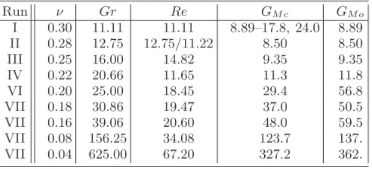
TABLE I: Parameters used in the simulations. GM c is the

critical magnetic Grashof that the dynamo instability begins and GM o is the critical magnetic Grashof that the dynamo

instability stops having on-off behavior. Thus, on-off inter-mittency is observed in the range GM c< GM < GM o.

Run ν Gr Re GM c GM o I 0.30 11.11 11.11 8.89–17.8, 24.0 8.89 II 0.28 12.75 12.75/11.22 8.50 8.50 III 0.25 16.00 14.82 9.35 9.35 IV 0.22 20.66 11.65 11.3 11.8 VI 0.20 25.00 18.45 29.4 56.8 VII 0.18 30.86 19.47 37.0 50.5 VII 0.16 39.06 20.60 48.0 59.5 VII 0.08 156.25 34.08 123.7 137. VII 0.04 625.00 67.20 327.2 362.

FIG. 2: Critical magnetic Grashof number GM c that the

dy-namo instability is observed (solid line) and the critical mag-netic Grashof number GM owhere the on-off intermittency is

disappears (dashed line).

Grashof number the critical magnetic Grashof number GMcis found and recorded in table I. For our lowest

kine-matic Grashof number Gr = 11.11 which corresponds to a slightly smaller value than the critical value that hy-drodynamic instabilities are present, the flow is laminar and the two windows of dynamo instability [43, 44] are rediscovered, shown in fig. 2. At higher Grashof number, the hydrodynamic system is not stable anymore, and the two dynamo window mode disappear, to collapse in only one (see fig.2). The critical magnetic Reynolds number is increasing with the Grashof (Reynolds) number fig.2, and saturates at very large values of Gr [55] that are far beyond the range examined in this work.

B. Route to the On-Off intermittency

The first examined Grashof number beyond the lami-nar regime is Gr = 12.75 (run II). In this case two sta-ble solutions of the Navier-Stokes co-exist. Depending of the initial starting condition, this hydrodynamic system

4

FIG. 3: Kinetic (inset) and magnetic energy for the run with Gr = 12.75 and GM = 22.32 for two runs starting with

dif-ferent initial conditions for the velocity field. The first flow (solid line) is attracted to the laminar ABC flow and gives no dynamo the second flow (dashed line) is attracted to a new solution that gives dynamo.

converges into one of the two attractors. The two veloc-ity fields have different critical magnetic Grashof num-bers. The first solution is the laminar flow that shares the same dynamo properties with the smaller Grashof number flows. For the second flow however the previous stable window between GM ≃ 17.8 and GM = 24.0

dis-appears and the critical magnetic Grashof number now becomes GMc = 8.50, resulting in only one instability

window. Figure 3 demonstrates the different dynamo properties of the two solutions. The evolution of the ki-netic and magki-netic energy of two runs is shown with the same parameters Gr, GM but with different initial

con-ditions for the velocity field. GM is chosen in the range

of the no-dynamo window of the laminar ABC flow. This choice of Gr although it exhibits interesting be-havior does not give on-off intermittency since both hy-drodynamic solutions are stable in time. The next exam-ined Grashof number (III), gives a chaotic behavior of the hydrodynamic flow and accordingly a “noisy” exponen-tial growth rate for the magnetic field. The evolution of the kinetic energy and the magnetic energy in the kine-matic regime is shown in fig. 4 for a relatively short time interval. The kinetic energy “jumps” between the values of the kinetic energy of the two states that were observed to be stable at smaller Grashof numbers in a chaotic manner. Accordingly the magnetic energy grows or decays depending on the state of the hydrodynamic flow, in a way that very much resembles a biased random walk in the log-linear plane. Thus, this flow is expected to be a good candidate for on-off intermittency that could be modeled by the SDE model equations given in eq.1. However this flow did not result in on-off intermittency for all examined magnetic Grashof numbers, even for the runs that the measured growth rate and amplitude of the noise were found to satisfy the criterion a/D < 1 for the existence of on-off intermittency. What is found

FIG. 4: The evolution of the kinetic (top panel) and magnetic (bottom panel) energy for the run with Gr = 16.0 and GM =

9.39.

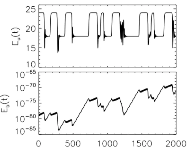
FIG. 5: The evolution of the magnetic energy for the run with Gr = 16.0 and GM = 9.39. At the linear stage the logarithm

of the magnetic energy grows like a random walk. At the nonlinear stage however the solution is trapped in a stable time periodic solution. The inset shows the evolution of the magnetic energy in the nonlinear stage in a much shorter time interval. The examined run has a/D = 0.022 < 1.

instead is that at the linear stage the the magnetic field grows in a “random” way but in the nonlinear stage the solution is “trapped” in a stable periodic solution and remains there throughout the integration time. This be-havior is demonstrated in fig. 5 where the evolution of the magnetic energy is shown both in the linear and in the non-linear regime. ‘

An other interesting feature of this flow is that ex-hibits subcriticality [25]. The periodic solution that the dynamo simulations converged to in the nonlinear stage appears to be stable even for the range of GM that no

dynamo exists. Figure 6 shows the time evolution of two runs with the same parameters Gr, GM one starting with

very small amplitude of the magnetic field and one start-ing usstart-ing the output from one of the successful dynamo runs in the nonlinear stage. Although the magnetic en-ergy of the first run decays with time the nonlinear

solu-FIG. 6: Subcritical behavior of the ABC dynamo. The evo-lution of the magnetic energy for two runs with Gr = 16.0 and GM = 9.30 starting with small amplitude magnetic field

(bottom line) and starting with an amplitude of the magnetic field at the nonlinear stage (top almost straight line).

tion appears to be stable.

The next examined Grashof number G = 20.66 (IV) appears to be a transitory state between the previous example and on-off intermittency that is examined in the next section. Figure 7 shows the evolution of the magnetic energy for three different values of GM =

20.66, 12.0, 11.6 for all off which the ratio a/D was mea-sured and was found to be smaller than unity and there-for are expected to give on-off intermittency based on the SDE model. Only the bottom panel however (which cor-responds to the value of GM = 11.6 closest to the onset

value GM = 11.3) shows on-off intermittency. A

singu-lar power law behavior of the pdf of the magnetic energy during the off phases (small Eb) for the last run was

ob-served to be in good agreement with the predictions of the SDE. This is expected since for small Eb the Lorentz

force that is responsible for trapping the solution in the nonlinear stage does not play any role.

C. On-off intermittency

All the larger Grashof numbers examined display on-off intermittency and there is no trapping of the solutions in the “on” phase. Figure 8 shows an example of the on-off behavior for Gr = 25.0 and three different values of GM ( GM = 41.6 (top panel), GM = 35.7 (middle panel),

GM = 31.2 (bottom panel)). As the critical value of GM

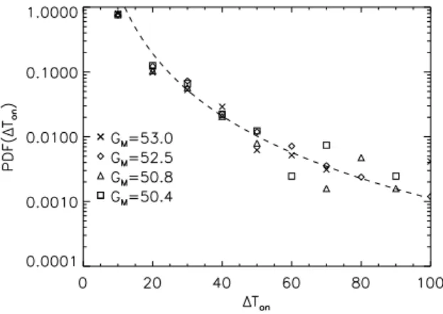
is approached the “on” phases of the dynamo (bursts) become more and more rare as the SDE model predicts. Note however that the “on” phases of the dynamo last considerably long. In fact the distribution of the dura-tion of the “on” phase ∆Ton is fitted best to a power

law distribution rather than an exponential that a ran-dom walk model with an upper no-flux boundary would predict, as can be seen in fig. 9.

FIG. 7: Evolution of the magnetic energy for Gr = 20.66 and GM = 20.66 (top panel), GM = 12.0 (middle panel),

GM = 11.6 (bottom panel).

FIG. 8: Evolution of the magnetic energy for Gr = 20.66 and GM = 20.66 (top panel), GM = 12.0 (middle panel),

GM = 11.6 (bottom panel).

FIG. 9: Distribution of the “on” times for the Gr = 39.06 case and three different values of GM. The fit (dashed line)

corresponds to the power-low behavior ∆T−3.2_{. Here ”on”}

time is considered the time that dynamo has magnetic energy Eb> 0.2.

6

FIG. 10: The probability distribution functions of Eb, for

Gr = 25 and and seven different values of GM (starting from

the top line: GM = 31.2, GM = 33.3, GM = 35.7, GM =

38.4, GM = 41.6, GM = 50.0, GM = 83.3. The last case

GM = 83.3 shows no on-off intermittency. The dashed lines

shows the prediction of the SDE model. The pdfs have not been normalized for reasons of clarity.

The effect of the long duration of the “on” times can also be seen in the pdfs of the magnetic energy. The pdfs for the Gr = 20.66 for the examined Gr are shown in figure 10. For values of GM much larger from the critical

value GMcthe pdf of the amplitude of the magnetic field

is concentrated at large values Eb≃ 1 producing a peak

in the pdf curves. As GM is decreased approaching GMc

from above a singular behavior of the pdf appears with the pdf having a power law behavior ∼ E−γ

b for small Eb.

The closer the GM is to the critical value the singularity

becomes stronger. The dashed lines show the prediction of the SDE model γ = 1 − a/D. The fit is very good for small Eb, however the SDE for a supercritical bifurcation

fails to reproduce the peak of the pdf at large Eb, that is

due to the long duration of the “on” phases.

An other prediction of the SDE model is that all the moments of the magnetic energy hEm

b i =

R P DF (Eb)EbmdEb have a linear scaling with the

devia-tion of GM from the critical value GMcprovided that the

difference GM− GMc is sufficiently small. This result is

based on the assumption the singular behavior close to Eb = 0 gives the dominant contribution to the pdf that

is always true provided that the ratio a/D is sufficiently small. However if the system spends long times in the “on” phase the range of validity of the linear scaling of hEbi with a ∼ GM− GMcis restricted to very small

val-ues of the difference GM − GMc. Figure 11 shows the

time averaged magnetic energy hEbi as a function of the

relative difference (GM − GMc)/GM in a log-log scale.

The dependence of hEbi on the deviation of GM from

the critical value appears to approach the linear scaling albeit very slow. The best fit from the six smallest values of GM shown in the fig.11 gave an exponent of 0.8 (e.g

hEbi ∼ (GM − GMc)0.8). The small difference from the

linear scaling (hEbi ∼ (GM−GMc)1) is probably because

FIG. 11: Averaged magnetic energy as function of the rel-ative deviation from the critical magnetic Grashof num-ber. The dash-dot vertical line indicates the location of (GM o_{− G}M c)/GM beyond which On-Off intermittency is no

longer present.

not sufficiently small deviations (GM− GMc) were

exam-ined. We note however that there is a strong deviation from the linear scaling for values of GM close to GMo.

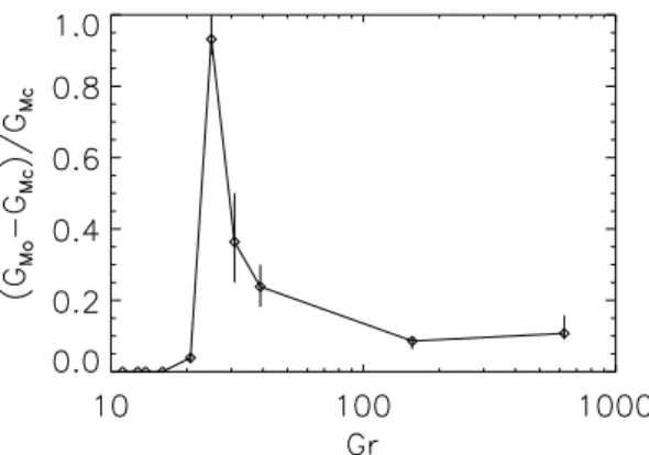
Of particular interest to the experiments is how the range of intermittency changes as Gr is increased. Typ-ical Gr numbers for the experiments are of the order of Gr ∼ Re2

∼ 1012

that is not currently possible to be obtained in numerical simulations. In figure 2 we showed the critical magnetic Grashof number GMc that

dynamo instability is observed and the critical magnetic Grashof number GMo that the on-off intermittency is

present. GMc was estimated by interpolation between

the run with the smallest positive growth rate and and the run with the smallest (in absolute value) negative growth rate. The on-off intermittency range was based on the pdfs of the magnetic energy. Runs that the pdf had singular behavior at Eb ≃ 0 are considered on-off while

runs with smooth behavior at Eb ≃ 0 are not considered

to show on-off intermittency. The slope of the pdfs (in log-log scale) for small Eb were calculated and the

tran-sition point GMo was determined by interpolation of the

two slopes (see for example the bottom two curves in fig. 10). In figure 12 we show the ratio (GMo− GMc)/GMc

as a function of Grthat expresses the relative range that

on-off intermittency is observed. The error-bars corre-spond to the smallest examined values of GM that no

on-off intermittency was observed (upper error bar) and the largest examined values of GM that on-off

intermit-tency was observed (lower error bar). The range of on-off intermittency is decreasing as Gr is increased probably reaching an asymptotic value. However to clearly de-termine the asymptotic behavior of GMo with Gr would

require higher resolutions that the long duration of these runs does not allow us to perform.

IV. DISCUSSION

In this work we have examined how the on-off intermit-tency behavior of a near criticality dynamo is changed as the kinematic Reynolds is varied, and what is the effect of the Lorentz force in the non-linear stage of the dynamo. The predictions of [30, 31, 32, 33], linear scaling of the averaged magnetic energy with the deviation of the con-trol parameter from its critical value, fractal dimensions of the bursts, distribution of the “off” time intervals, and singular behavior of the pdf of the magnetic energy that were tested numerically in [21, 22] were verified for a larger range of Kinematic Grashof numbers when On-Off intermittency was present. Note however that all these predictions are based on the statistics of the flow in the kinematic stage of the dynamo. However it was found that the Lorentz force can drastically alter the On-Off be-havior of the dynamo in the non-linear stage by quench-ing the noise. For small Grashof numbers the Lorentz force can trap the original chaotic system in the linear regime in to a time periodic state resulting to no On-Off intermittency. At larger Grashof numbers Gr > 20 On-Off intermittency was observed but with long durations of the “on” phases that have a power law distribution. These long “on” phases result in a pdf that peaks at fi-nite values of Eb. This peak can be attributed to the

presence of a subcritical instability or to the quenching of the hydrodynamic “noise” at the nonlinear stage or possibly a combination of the two. In principle the SDE model (eq.1) can be modified to include these two effects: a non-linear term that allows for a subcritical bifurcation and a Ebdependent amplitude of the noise. There many

possibilities to model the quenching of the noise, however the nonlinear behavior might not have a universal behav-ior and we do not attempt to suggest a specific model.

FIG. 12: The ratio (GM o_{− G}M c)/GM c as a function of Gr

that expresses the relative range that on-off intermittency is observed. Error-bars correspond to the smallest examined values of GM that no on-off intermittency was observed

(up-per error bar) and the largest examined values of GM that

on-off intermittency was observed (lower error bar).

The relative range of the On-Off intermittency was found to decrease as the Reynolds number was increased possibly reaching an asymptotic regime. However the limited number of Reynolds numbers examined did not allow us to have a definite prediction for this asymptotic regime. This question is of particular interest to the dy-namo experiments [2, 3, 4, 5, 6, 7, 8] that until very recently [26] have not detected On-Off intermittency . There are many reasons that could explain the absence of detectable On-Off intermittency in the experimental setups, like the strong constrains imposed on the flow [4, 5] that do not allow the development of large scale fluctuations or the Earths magnetic field that imposes a lower threshold for the amplitude of the magnetic energy. Numerical investigations at higher resolution and a larger variety of flows or forcing would be useful at this point to obtain a better understanding.

Acknowledgments

We thank F. P´etr´elis, J-F Pinton for fruitful dis-cussions. AA acknowledge the financial support from the “bourse Poincar´e” of the Observatoire de la Cˆote d’Azur and the Rotary Club district 1730. YP thank CNRS Dynamo GdR, INSU/PNST, and INSU/PCMI Programs. Computer time was provided by IDRIS, and the Mesocentre SIGAMM machine, hosted by Observa-toire de la Cote d’Azur.

8

[1] H. K. Moffatt, Magnetic Field Generation in Electrically Conducting Fluids Cambridge University Press, Cam-bridge, (1978) ; F. Krause and K.-H.Radler, Mean-Field Magnetohydrodynamics and Dynamo Theory Pergamon, Oxford,(1980) ; E. N. Parker, Cosmical Magnetic Fields Clarendon, Oxford, 1979.

[2] A. Gailitis, et al., Phys. Rev. Lett. 84, 4365 (2000). [3] A. Gailitis, et al., Phys. Rev. Lett. 86, 3024 (2001). [4] A. Gailitis, et al., Physics of Plasmas 11 Issue 5, 2838–

2843 (2004).

[5] U. Muller and R. Stieglitz, Naturwissenschaften 87, 381 (2000).

[6] R. Stieglitz and U. Muller, Phys. Fluids 13, 561 (2001). [7] R. Monchaux et al., Phys. Rev. Lett. 98, 044502 (2007). [8] M. Berhanu et al., Europhys. Lett. 77, 59001 (2007). [9] P. Odier, J.-F. Pinton, S. Fauve Phys. Rev. E 58, 7397–

7401 (1998).

[10] N. L. Peffley, A. B. Cawthorne, and D. P. Lathrop, Phys. Rev. E 615287 (2000).

[11] N. L. Peffley et al Geoph. J. Int. 142, 52–58 (2000). [12] P. Frick et al, Magnetohydrodynamics 38 No. 1/2, 143–

162, (2002).

[13] M. Bourgoin et al Phys. Fluids 14, 3046 (2002). [14] M. D. Nornberg, E. J. Spence, R. D. Kendrick, C. M.

Jacobson, and C. B. Forest, Phys. Rev. Lett. 97, 044503 (2006).

[15] M. D. Nornberg et al Phys. Plasmas 13, 055901 (2006). [16] R. Stepanov, R. Volk, S. Denisov, P. Frick, V. Noskov,

and J.-F. Pinton Phys. Rev. E 73, 046310 (2006). [17] R. Volk, P. Odier, and J-F Pinton, Phys. Fluids bf 18

085105 (2006).

[18] M. Bourgoin et al New Journal of Physics 8, 329 (2006). [19] Y. Pomeau and P. Manneville, Commun. Math. Phys.

74, 1889 (1980).

[20] N. Platt, E. A. Spiegel and C. Tresser, Phys. Rev. Lett. 70(3), 279–282 (1993).

[21] D. Sweet, E. Ott, J. M. Finn, T. M. Antonsen, Jr. and D. P. Lathrop Phys. Rev. E, 63, 066211 (2001).

[22] D. Sweet, E. Ott, T. M. Antonsen, Jr. and D. P. Lathrop, J. M. Finn Physics of Plasmas 8, 1944–1952 (2001). [23] A. S. Pikovsky,Z. Phys. B 55, 149 (1984); P.W. Hammer,

N. Platt, S.M. Hammel, J.F. Heagy and B.D. Lee Phys. Rev. Lett. 73(8), 1095–1098 (1994). T. John, R. Stannar-ius and U. Behn, Phys. Rev. Lett. 83 (4), 749–752 (1999). D.L. Feng, C.X. Yu, J.L. Xie, W.X. Ding, Phys. Rev. E 58(3), 3678–3685 (1998). F. Rodelsperger, A. Cenys and H. Benner, Phys. Rev. Lett. 75 (13), 2594–2597 (1995). [24] N. Leprovost, B. Dubrulle, F. Plunian,

Magnetohydrody-namics 42131–142 (2006).

[25] Y. Ponty, J.-P. Laval , B. Dubrulle, F. Daviaud, J.-F. Pinton Phys. Rev. Lett., under press. arXiv:0707.2498 [26] VKS Private communication, Les Houches, August 2007. [27] H. Fujisaka and T. Yamada, Prog. Theor. Phys. 74 (4), 918–921 (1984). H. Fujisaka, H. Ishii, M. Inoue and T.

Yamada, Prog. Theor. Phys. 76 (6), 1198–1209 (1986). [28] E. Ott and J. C. Sommerer,Phys. Lett. A 188, 39 (1994). [29] L. Yu, E. Ott, and Q. Chen, Phys. Rev. Lett. 65, 2935

(1990).

[30] N. Platt, S. M. Hammel, and J. F. Heagy, Phys. Rev. Lett. 72, 3498 (1994).

[31] J. F. Heagy, N. Platt, and S. M. Hammel, Phys. Rev. E 49, 1140 (1994).

[32] S. C. Venkataramani, T. M. Antonsen, Jr., E. Ott, and J. C. Sommerer, Phys. Lett. A 207, 173 (1995) . [33] S. C. Venkataramani, T. M. Antonsen, Jr., E. Ott, and

J. C. Sommerer, Physica D 96, 66 (1996).

[34] S. Aumaˆitre, F. P´etr´elis, and K. Mallick, Phys. Rev. Lett. 95, 064101 (2005).

[35] S. Aumaˆitre, K. Mallick and F. P´etr´elis, Journal of Sta-tistical Physics, 2006, 123, 909–927 (2006).

[36] F. Cattaneo, D.W. Hughes and E.J. Kim, Phys. Rev. Lett. 76, 2057-2060 (1996).

[37] E. Zienicke, H. Politano and A. Pouquet, Phys. Rev. Lett. 81, 4640-4640 (1998).

[38] N.H. Brummell, F. Cattaneo , S.M. Tobias Fluid Dynam-ics Research 28, 237-265 (2001).

[39] V. I. Arnold, Comptes Rendus Acad. Sci. Paris 261, 17 (1965).

[40] T. Dombre, U. Frisch, J. M. Greene, M. Henon, A. Mehr, and A. Soward, J. Fluid Mech. 167, 353 (1986). [41] Galloway, D.J. and Proctor, M.R.E. Nature 356, 691–693

(1992).

[42] Y. Ponty, A. Pouquet and P.L. Sulem, Geophys. Astro-phys. Fluid Dyn.79, 239-257 (1995).

[43] V.I. Arnold, and E.I. Korkina, Vestn. Mosk. Univ. Mat. Mekh. 3, 43–46 (1983).

[44] Galloway, D.J. and Frisch, U., Geophys. Astrophys .Fluid Dyn. 36, 53–83 (1986).

[45] B.Galanti, P. L. Sulem and A. Pouquet, Geophys. Astro-phys .Fluid Dyn. 66, 183–208 (1992).

[46] V. Archontis, S.B.F. Dorch and A. Nordlund, Astron. Astrophys. 397, 393-399 (2003).

[47] R. Teyssier, S. Fromang and E Dormy J. Comp. Dyn. 21844–67 (2006).

[48] S. Childress and A.D. Gilbert, “Stretch, Twist Fold: The Fast Dynamo”, Springer-Verlag, New York (1995). [49] H. K. Moffat and M. R. Proctor, J. Fluid Mech. 154, 493

(1985).

[50] B. J. Bayly and S. Childress, Geophys. Astrophys. Fluid Dyn. 44, 211 (1988).

[51] J. M. Finn and E. Ott Phys. Fluids 31, 2992 (1988). [52] John M. Finn and Edward Ott Phys. Rev. Lett. 60, 760

(1988).

[53] O.M. Podvigina and A. Pouquet, Physica D 75, 471-508 (1994):

[54] O.M. Podvigina Physica D 128, 250-272 (1999). [55] P. D. Mininni Physics of Plasmas 13 (5), 056502 (2006).