Dispersion compensation for reflection holography

(1)

Dispersion Compensation

for

Reflection Holography

by Arno Klein

B.S., Perception and Cognition Studies University of Michigan in Ann Arbor, 1993 Submitted to the Program in Media Arts and Sciences,

School of Architecture and Planning

in partial fulfillment of the requirements for the degree of Master of Science in Media Arts and Sciences

at the

Massachusetts Institute of Technology September 1996

Signature of Author

Program in kedia Arts and Sciences June 15, 1996

Certified by

Stephen A. Benton

Allen Professor of Media Arts and Sciences Program in Media Arts and Sciences

Thesis Supervisor

Accepted by

F 7!

vStephen A. Benton Chair

Departmental Committee on Graduate Students Program in Media Arts and Sciences

(2)

(3)

Dispersion Compensation

for Reflection Holography

by Arno Klein

Submitted to the Program in Media Arts and Sciences, School of Architecture and Planning

on June 15, 1996 in partial fulfillment of the requirements for the Degree of Master of Science in Media Arts and Sciences ABSTRACT

The work outlined in this thesis is the exploration, application, and evaluation of the technique of dispersion compensation to reduce color blurring of reflection

holograms. In particular, the technique of illuminating a hologram with a predispersing grating is applied to the development of full-color, full-parallax, reflection holographic stereograms in various display formats, from a large, open-air viewstation to a compact, light guide-mounted hologram. The effects of wave-front curvature are assessed for reducing the grating size for more compact displays.

A blur equation is derived and experimentally contrasted with Benton's blur equations with the use of spectrophotometer measurements of an experimental grating, and raytracing computer programs included in the appendices.

Finally, two approaches were developed that provide a consistent means of designing dispersion-compensation gratings tailored to realizable, desired geometries. Both approaches are effectively reverse-raytracing methods, beginning from the pupil and ending at the extended light source. Compensation is optimized for image points along a prescribed viewing axis, and depending on the geometry, along all lines of sight parallel to this axis. The first approach solves for a grating design where the grating is

reconstructed with the same angles to which it was exposed. The second, more exact approach, is an optimization of a matrix expression containing the relevant angular and/or vertical focus equations, using the Moore-Penrose pseudoinverse function. This latter method will enable the reader to design a grating that will play out at the desired angles for component wavelengths at as close to the desired distances as possible.

Thesis Supervisor: Stephen A. Benton

(4)

(5)

Dispersion Compensation for Reflection Holography

The following people served as readers for this thesis:

Certified by

Edward Adelson

Associate Professor of Vision Science

Certified by

Stephen D. Fantone

Senior Lecturer, Mechanical Engineering President, Optikos Corp., Cambridge, MA

Certified by _

Emmett N. Leith

Professor of Electrical Engineering and Computer Science

(6)

(7)

(8)

(9)

Acknowledgments

This section is inevitably going to be woefully incomplete, so I will mention only the names of those who have had a direct impact on the production of this thesis.

First, I would like to thank Steve Benton, for the opportunity to work in the Media Laboratory, and for his extremely helpful e-mail correspondence.

Sincere thanks also goes to my other thesis readers for reviewing this document: Professor Ted Adelson, Professor Stephen Fantone, and Professor Emmett Leith.

The Spatial Imaging Group, as of spring, 1996:

Mike Klug, the other primary individual constituting the "we" that is used

throughout the thesis. Mike shot the holograms illuminated by the gratings, and pulled together all elements to complete the viewstations for our sponsors. My reluctant lab mentor: "Don't you have a thesis to work on?"

Ravi Pappu, my colleague and cohort, for fielding my math questions, however far afield: "On what planet does sine of zero equal one?!" Thank you for bearing the innumerable intrusions!

Paul Christie, my 6th and longest-lasting officemate, for sharing my abode:

"It would probably be safer if you'd sleep farther away from the door." Have a wonderful wedding!

Melissa Yoon, for countless administrative feats: "The package should have arrived in England this morning - Anything more you'd like to Fedex today?"

Take care and good luck with your (near) future endeavors...

Wendy Plesniak, for inspirational work that adds touch to an otherwise ghostly medium. Carlton Sparrell: "You didn't know? I'm leaving in two weeks."

Michael Halle

Our undergraduate researchers; in particular, Adam Kropp and Benjie Chen, for their computer graphics work instrumental to providing the subjects of our holograms. John Sutter, our Japanese affiliate

Barrett Comiskey, director of darkroom #2, my friend, roommate, and fellow holographer: "Your thesis is my thesis."

Mitch Henrion, for edgelit enthusiasm.

Everyone in the Physics and Media Group, for providing me with a friendly place to work on my thesis round the clock.

Steve Mackara, Kirk Steijn, and Bill Gambogi of DuPont.

Steve Mackara was kind enough to shoot the master grating and some contact copies for the final viewstations of Chapter 5.

Kirk Steijn was very helpful in providing TK Solver information.

(10)

Sincere gratitude to those who have supported my work in the past:

My family

Jason Smith, my close friend and holography partner since high school, for his shared vim, vigor, and vitality.

Kashiko Kodate and Katsuma-sensei, who made it possible for me to do independent holography work in Japan.

Professor Emmett Leith once again, for his generous offer to use his facilities during my stay at the University of Michigan: "Here comes the night shift."

Helpful discussions, distractions:

Professor Seth Teller, for discussions, not distractions.

Ranjana Mitra, my mutual distraction: "I know you've got a thesis, but do you want to scale some buildings tonight?"

David James, my personal D.J., for providing musical interludes from afar, such as The Blur! They helped me to get focused...

Kory and Ian - Congratulations, and I wish you all the best for your future together!

Text in this thesis was written on Microsoft Word for Windows 95, Version 7.0. Mathematics segments were written with Microsoft Equation 2.0,

and for Chapter 2, Mathcad 5.0+ (MathSoft Inc.).

Figures were drawn with Microsoft PowerPoint for Windows 95, Version 7.0. Graphs in Chapter 1 were made using Microsoft Excel for Windows 95, Version 7.0. Computer programs were written in:

TK Solver+, Version 1.2 (Universal Technical Systems), for the first program in Appendix 4.

Matlab (The Math Works, Inc.), for the programs of Appendices 5 and 6, and the second program in Appendix 4.

Dictation was performed for parts of the thesis, using Dragon Dictate (Classic Edition) for Windows, Version 2.01 (Dragon Systems, Inc.).

(11)

Page: 13 Extended Table of Contents Page: 17 List of Figures and Tables Page: 21 Introduction

Page: 23 Dispersion compensation flowchart Page: 25 1. Blur in holographic images

Page: 49 2. Trigonometric derivation of a single-plane blur equation Page: 65 3. Introduction to dispersion compensation

and a brief review of its application to holographic displays Page: 77 4. Full-parallax reflection holographic stereograms

Page: 85 5. Example design of a dispersion-compensated,

full-parallax holographic viewstation

Page: 97 _{6. Wave-front shapes, compact displays, and designing gratings} Page: 125 Conclusions and future work

Page: 129 Al. Single-plane trigonometric raytracing formulas Page: 133 A2. Derivation of a vector blur equation

and its reduction to the blur equation of Chapter 2 Page: 141 A3. TK Solver+ and Matlab programs

applying the derived equations Page: 155 A4. A Matlab program for the design of

dispersion-compensation gratings (Chapter 6)

Page: 159 _{A5. A Matlab program attempting to solve for a pre- and} post-dispersing grating set flush against a hologram (Chapter 6) Page: 161 References

(12)

(13)

Extended Table of

List of Figures and Tables

Please note that in the figures, holographic images that seem to float outside of the solid angle subtended by the observer's eyes and the hologram are merely for illustrative purposes. Visible image points must lie along a line of sight from the eye to the

hologram without the aid of smoke, mirrors, or re-emitting gases. Figure 1.1: Successive wave fronts emanating from a point source of light Figure 1.2: The Moire fringe pattern

Figure 1.3: The formation of a reflection hologram (after Jeong 1980) Figure 1.4: The reconstruction of a reflection holographic image (Jeong 1980) Figure 1.5: Interference pattern forming a Gabor zone plate

Figure 1.6: Spatial frequencies

Figure 1.7: Formation of a Gabor zone plate, with more closely spaced fringes toward its periphery (after Greivenkamp 1995)

Figure 1.8: Illumination of a Gabor zone plate with a single wavelength, with resulting virtual and real image points

Figure 1.9: Phase-conjugate illumination of a Gabor zone plate with a single wavelength Figure 1.10: Illumination of a Gabor zone plate with two wavelengths, and the resulting

longitudinal dispersion

Figure 1.11: The formation of an off-axis reflection hologram (after Jeong 1980) Figure 1.12: Reconstruction of an off-axis reflection hologram

Figure 1.13: Dispersion in an off-axis reflection hologram: illumination by two wavelengths Figure 1.14: Examples of different fringe patterns (Geisler and Banks, fig. 7.25.36-19)

Figure 1.15: Different acuity tests (Geisler and Banks, fig. 7.25.36-19) Figure 1.16: Stereoacuity

Figure 1.17: Airy disk diffraction pattern (Riggs 1965, fig. 11.10)

Figure 1.18: Rayleigh's criterion for just resolvable points (Riggs 1965, fig. 11.11) Figure 1.19: Two blurred points that are just resolvable

Figure 1.20: Photopic curve data from Wyszecki and Stiles (1967, table 4.2) Figure 1.21: Illuminant A curve (Wyszecki and Stiles 1967; MIT 1936)

Table 1.1: Data from the spectral luminous efficiency (Wyszecki and Stiles 1936) and Illuminant A relative intensity (MIT 1936) curves

Figure 1.22: Intensity filters: the retina and illuminant

Figure 1.23: Just resolvable points defined by the diffraction efficiency curve Figure 1.24: Perceived blur size factor

Figure 2.1: Spectral components from different points on the hologram contributing to blur Figure 2.2: Dispersed focus at the pupil, perceived as color blur, from Appendix 2 Figure 2.3: Perceived color blur and source-size blur height

Figure 2.4: Dispersion for the cases of m = +1 or m = -1 order image points combined in one diagram

Figure 2.5: The achromatic angle for the cases of m = +1 or m = -1 order image points combined in one diagram

Figure 2.6: Wavelength-dependent focusing power of a hologram, and the achromatic angle (Saxby 1992)

Figure 2.7: The perceived blur angle according to Benton (1994) Figure 2.8: (from Appendix 1)

Figure 2.9: Measurement 3 setup

(18)

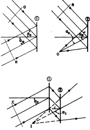
Figure 3.1: DeBitetto's original diagram discriminating the effects of diffraction orders on relative dispersion

Figure 3.2: Forward and reverse raytracing the spectral components through a transmission hologram Figure 3.3: Raytracing the dispersed rays from the hologram through a transmission grating

Figure 3.4: A schematic representing the original geometry of the three researchers in reverse (Latta 1972)

Figure 3.5: Single view angle dispersion compensation

This schematic represents the blurring of image points off of the local normal for a collimated reference /collimated illumination geometry.

Figure 3.6: Burckhardt's (1966) use of a louver film to block the zero order of the hologram in a single view angle dispersion-compensation display

Figure 3.7: Burckhardt's single viewpoint dispersion compensation technique (Collier, Burckhardt, and Lin 1971)

Figure 3.8: Example of the complexity of modern head-up displays incorporating dispersion-compensation gratings (Roberts, et al. 1995)

Figure 3.9: Bazargan's display, manufactured by Holoplex Systems, Ltd. (Syms 1990, fig. 10.5-2) Figure 3.10: Benton's patent drawing of the white-light transmission hologram transfer step (1972) Figure 3.11: Benton's patent drawing of the special achromatizing grating

used in an exposure step (1985)

Figure 3.12: (a) Distortions of a square image across the visible spectrum (400-700 nm)

(b) Single view angle dispersion compensation for reducing lateral chromatic aberration (Bazargan 1986, fig. 7.20)

Figure 3.13: Bazargan's suggested approach for making a full-color, dispersion-compensated display Figure 3.14: Kubota's reflection /reflection dispersion-compensated display

Figure 3.15: Intensity profile of the reconstructed image points

in Kubota's single view angle dispersion-compensation display Figure 4.1: Sequential images are taken, and later projected to expose

a hologram with an appropriately scaled geometry (Redman 1968). Figure 4.2: DeBitetto's original drawing of the spatial multiplexing technique

most commonly used in display holographic stereograms today (DeBitetto 1968) Figure 4.3: A horizontal-parallax-only holographic stereogram (HPO HS, or Hi)

Figure 4.4: The first (a) and last (b) vertical strip exposures of a holographic stereogram (top view) Figure 4.5: Transfer setup

Figure 4.6: Phase-conjugate illumination of the HPO HS H2, and reconstruction of an orthoscopic, real image

Figure 4.7: Benton's pseudocolor technique for producing achromatic or full-color images (1983, 1988) Figure 4.8: An example of different perspective views of a full-parallax hologram

(image care of Michael Klug)

Figure 5.1: Uncompensated and compensated dispersion of a holographic image Figure 5.2: Schematic of the final viewstation with tipped grating

Figure 5.3: Schematic of the exposure (2250) and illumination (450) geometries of the dispersion-compensated H2 (from Chapter 4)

Figure 5.4: The desired grating playout (450)

Figure 5.5: The required master grating exposure geometry (56.32' degrees), taking into account shrinkage of the photopolymer

Figure 5.6: The master grating exposure holographic table setup Figure 5.7: The transfer grating exposure holographic table setup Figure 5.8: filament orientation

Figure 5.9: Bulb with an ellipsoidal, dichroic reflector

(19)

Figure 6.1: Non-chromatic blurring of the edgelit hologram

Figure 6.2: Exposure of an edgelit hologram illuminated with the same source distance and folded beam path (Upatnieks 1992)

Figure 6.3: Reduction of chromatic and non-chromatic blurring of the edgelit hologram using a wave-front-shaping steep angle HOE

Figure 6.4: Upatnieks' achromatic edgelit hologram (1992)

Figure 6.5: A comparison of Birner's reflection HOE/transmission steep angle H2 with the author's reflection/reflection displays

Figure 6.6: Maximum acceptable perceived longitudinal blur length

Figure 6.7: Collimated, phase-conjugate, single view angle dispersion-compensated hologram with maximum depths (3 arc minutes of resolution):

Figure 6.8: Uncollimated, phase-conjugate, single view angle dispersion-compensated hologram with maximum forward compensated depths (1 arc minute of resolution)

Figure 6.9: Uncollimated, non-phase-conjugate, single view angle dispersion-compensated hologram with extreme field curvature (diverging/diverging geometry) Figure 6.10: Ideal predispersed hologram illumination angles and distances

should be equivalent to the ideal predispersed grating output angles. Figure 6.11: Exposure of the transfer (H2) hologram with a diverging reference source Figure 6.12: Reconstruction of the H2 with a diverging illumination source

Figure 6.13: The final table setup for the 750/750 diverging/diverging geometry

Figure 6.14: A graph of the exposure and illumination angles for a range of central output angles. This graph is the output from the Matlab 'plot' command in the program of Appendix 4. Figure A1.1: Grating vector cloud (Goodman, 1996)

Figure A1.2: Dispersion measurements with an Oriel spectrophotometer Table A1.1: Measurements of dispersion with an Oriel spectrophotometer

Figure A1.3: Diagram accompanying Benton's vertical focus equation derivation (Benton, 1994 Figure A2.1: Magnitudes and directions for the vector derivation of a blur equation

Figure A2.2: Trigonometric diagram

(20)

(21)

Introduction

"True observers of nature, however they may differ in opinion in other respects, will agree that all which presents itself as appearance, all that we meet with as phenomenon, must either indicate an original division which is capable of union, or an original unity which admits of division, and that the phenomenon will present itself accordingly. To divide the united, to unite the divided, is the life of nature; this is the eternal systole and diastole, the eternal collapsion and expansion, the inspiration and expiration of the world in which we live and move."

-- Goethe, Theory of Colours (1810, 293-4)

It is the sincere hope of the author that the following body of work, the result of a year of study, may serve as a helpful starting point for future researchers interested in the problems of image blur in holographic displays, and grating design. In order to expedite the reader's inquiry, this Introduction will serve as a brief outline of the contents of each chapter. The "Conclusions and future work" section will parallel this summary.

Chapter 1 consists of two parts: The first is an introduction to holography and dispersion, or color blur. In the second part, we will estimate the degree to which our perception of blur affects the resolution of a holographic image.

In Chapter 2, we derive and experimentally test a trigonometric blur equation for the absolute raytraced size of a blurred image. We then apply the perceived blur size factor from Chapter 1 to find the perceived size of this image. The author's blur equation is compared with Benton's blur equation.

In Chapter 3, we introduce dispersion compensation, a method to correct for color blur, and we give a brief history of the application of dispersion compensation to display holography.

Chapter 4 gives an introduction to full-parallax holographic stereograms, the particular type of hologram we will be illuminating in Chapter 5's display.

Chapter 5 is the culmination of the previous chapters' findings, applied to a plane-wave viewstation display. Laboratory techniques for forming a dispersion compensating grating are outlined here.

Chapter 6 compares the effectiveness of compact dispersion-compensation displays that do and do not use a plane-wave grating. Then, a consistent means for designing dispersion-compensation gratings is put forward in the chapter and in the accompanying computer programs of Appendices 3 and 4. It is shown that the method presented here (the use of the Moore-Penrose pseudoinverse) compares favorably with the perfect reconstruction geometries implemented in the viewstations of Chapters 5 and 6 and is well-suited to finding optimized angles, and also approximate distances, with less precision. It therefore is tailored to compensate for lateral and longitudinal dispersion as a function of eye position and orientation.

(22)

(23)

Dispersion compensation flowchart

Hologram view angle with optimized compensation

Hologram illumination angles for a given bandwidth

Ideal grating output angles, distances

Exposure geometry for perfect reconstruction, ideal and with grating tilt

3.1, 6.9, 6.13, A3

6.9, 6.13, A3

Optimizing grating designs for ideal angular and distance playout (imperfect reconstruction) 5.3, 6.13, A3 6.9-6.11, 6.14, A4 5.1-5.2 Ch. 5, 6 5.4 6.1-6.2 6.3, 6.5-6.8, 6.12, A4

The numbers next to the boxes represent relevant sections. 5.3, 6.12-6.13

(24)

(25)

Chapter 1 Blur in holographic images

1.1 Blur in holographic images

The primary sources of blur in holographic images are the spectral width and physical size of the illumination source, as well as non-ideal properties of the exposure medium and substrate. For full-parallax1 holographic displays with controlled lighting conditions, the spectral width usually constitutes the greatest source of image blur, and as

such will comprise the bulk of our discussions. As most optical aberrations have a chromatic component, we will refer to the blur due to polychromatic illumination simply

as "color blur." In this first chapter, we will introduce blur as we cover basic principles of holography. Then we will determine how our perception of blur affects the resolution

of a holographic image.

Because holograms rely on diffraction, and diffraction is wavelength dependent (that is, red wavelengths will deflect at greater angles through diffractive media than will blue wavelengths), a single holographically recorded object replays in a different location

for each component wavelength of the illumination. This separation of component wavelengths, or dispersion, is analogous to the phenomenon of dispersion in refractive media, such as a prism. The extent of the spectral width of the source determines the extent to which light will disperse through a given medium, and therefore a broadband white light source can render an image an indistinguishable rainbow blur.

One trivial solution to the problem of color smearing of images is to illuminate the hologram instead with a very narrow spectral band source, such as a laser or an arc lamp with an interference filter. These are impractical for most viewing situations and, unless one sets up three such lamps, offer only monochromatic playback. Another solution is to produce better recording materials or to find better processing methods for producing more narrow band playout. In either case, whether a hologram is illuminated by a narrow spectral band source or a hologram with a narrow band playout is illuminated by an intense broad band source, much of the illumination light is wasted. To produce brighter, full-color, full-parallax holograms that are sharp and deep, correcting for color blur in white light illumination displays is vital.

1 "Full-parallax" refers to the change in perspective vertically as well as horizontally. Synthetic full-parallax holograms are the subject of Chapter 5.

(26)

1.2 Basic principles of holography

To better understand color blur, we will take a brief look at some basic

interference patterns, and then invoke the limiting case of the first type of hologram that was invented by Dennis Gabor in 1947 (Gabor 1948). If we have a source point acting as

a harmonic oscillator, radiating waves in three dimensions, we can represent the

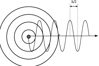
instantaneous wave fronts emanating from the center as concentric spheres, whose radii are incremented by one-half of a wavelength (/2). The direction of travel for any point on the wave front is simply the direction of expansion, the local normal to the sphere (Figure 1.1). We will call the path the light's direction takes a ray, and tracing its path is called raytracing.

/2

(27)

The superposition of two such wave fronts results in an interference pattern of hyperboloidal surfaces:

Figure 1.2: The Moire fringe pattern is a helpful visual aid to understanding interference effects2. Here we have the oscillating source above in isolation, and interfering with another source.

(a) The spherical wave fronts from a single light source (b) The superposition of wave fronts from two light sources

(c) The interference pattern created by the two sources (Jeong 1980)

If the two sources are mutually coherent then this interference pattern will remain constant over time, a "standing wave." We may place a

photosensitive recording material anywhere in the volume of space around or between these two sources to record the interference pattern. If placed between the two sources, the recording material will subsequently form partially reflective, hyperboloidal surfaces

spaced through its volume:

2 For and in-depth look into the analogy between moire fringe patterns and interference fringes, Abramson's book (1981) is an invaluable guide. A summary table may be found on page 9 of the book.

(28)

Figure 1.3: The formation of a reflection hologram (after Jeong 1980)

If the fringe pattern in this recording material retains its structural integrity and is then re-illuminated by a wave front from one of these two sources, this wave front will be partially reflected off each hyperboloidal surface and will interfere with itself. The interference determines the intensity of the light reflected off these surfaces in different directions. Light will be reinforced more in some directions than in other directions. Light traveling in directions corresponding to the directions light traveled from the other source during exposure are constructively interfered, and a reflection holographic image of the other source position will be formed (Figure 1.4).

Figure 1.4: The reconstruction of a reflection holographic image (Jeong 1980) The illumination source point is to the right, the reconstructed image to the left.

(29)

1.3 The Gabor zone plate

The particular interference pattern pictured in Figure 1.3, formed by source points on a line (the optical axis) intersecting the recording material, is called a "Gabor zone plate," or "in-line" hologram. If we had set the recording material along the optical axis, but not in between the two source points, a different form of Gabor zone plate would be formed, an in-line transmission hologram:

Figure 1.5: Interference pattern forming a Gabor zone plate

The interference pattern of the in-line transmission hologram is composed of concentric circles centered around the axis. Because the angle between the line containing the source points and the axis is zero, so too is the corresponding fringe density, or spatial frequency3 of the interference pattern. The angle between these two points with respect to a point on the hologram off-axis increases toward the edges, and the corresponding spatial frequency increases (See Figures 1.6 and 1.7).

3 Spatial frequency refers to the reciprocal of the distance between elements of a repeated pattern, such as

holographic fringes: f = sin(Ore)- , in cycles/mm.

A = wavelength

(30)

(a) (b)

(b) -. z

Figure 1.6: As the apparent distance between source points increases, so too does the spatial frequency of the fringes. In this figure, we are looking at the two sources from two different points on the recording material, one point close to the optical (z-) axis (a), another farther off-axis (b).

(31)

z

Figure 1.7: Formation of a Gabor zone plate, with more closely spaced fringes toward its periphery (after Greivenkamp 1995)

Because the center of the zone plate has zero spatial frequency4_{, light illuminating}

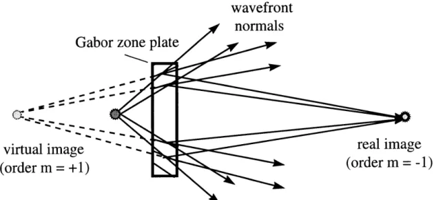
the hologram on axis will pass through undiffracted. Diffractive, or focusing power increases with increasing spatial frequency, so the zone plate's edges deflect incident light the most, in the direction of the original wave front from the other source point, as well as toward a focused, real image point in front of the observer. This second image in line with the first, is sometimes referred to as a "twin image." In Figure 1.8, the twin image is a real, focused image.

4 _{There may or may not be a fringe in the center of a transmission in-line hologram, depending on the}

relative phase of the two exposure beams. The reflection in-line hologram has fringes parallel with the surface. In either case, the center of the zone plate has no diffractive power for on-axis rays.

(32)

wavefront

normals

Gabor zone plate

virtual image

real image

(order m = +1)

(order m

=

-1)

Figure 1.8: Illumination of a Gabor zone plate with a single wavelength, with resulting virtual and real image points

Phase-conjugate illumination is essentially a reversal of the directions of the rays that exposed the hologram. This "time-reversed" illumination results in a real image point projected where the original object point was located. Here, the twin image is a virtual image behind the hologram plane from the observer (Figure 1.9).

real image

virtual image

(order m

=

-1)

(order m

=

+1)

Figure 1.9: Phase-conjugate illumination of a Gabor zone plate with a single wavelength 1.4 Longitudinal and lateral dispersion

As the spacing of between the fringes determines what wavelengths will

constructively interfere at different angles, it is possible to produce another image point at a different location by illumination with a different wavelength. The focusing power is therefore not only a function of spatial frequency, but also of wavelength, and therefore the wavelengths illuminating a Gabor zone plate focus to different points along the axis. The color blur of the longitudinally displaced images of the source points is termed longitudinal color blur and is not noticeable by an observer situated along this axis. If, however, the observer moves off the axis, the color blur becomes quite apparent.

(33)

BR

R

dispersed

virtual image

points

dispersed

real image

points

Figure 1.10: Illumination of a Gabor zone plate with two wavelengths, red (R) and blue (B), and the resulting longitudinal dispersion

Likewise, if we take a source point off-axis during recording of the hologram, white-light illumination of the hologram will result in lateral color blur. This off-axis hologram, invented by Leith and Upatnieks (1962), can eliminate the twin image so that the observer sees only one image.

Figure 1.11: The formation of an off-axis reflection hologram (after Jeong 1980)

Chapter 1: Blur in holographic images

(34)

-

.11.

Figure 1.12: Reconstruction of an off-axis reflection hologram, where the twin image is eliminated. The illumination source point

is to the right, and the virtual image is to the left.

Figure 1.13: Dispersion in an off-axis reflection hologram: The broad band illumination source point to the right results in Red and Blue image points to the left.

(35)

The lateral color blur may be explained by the fact that the source points are laterally displaced, creating a different interference pattern, and therefore the off-axis white light illumination of the hologram will focus points of different colors so that they are laterally displaced, as well as longitudinally displaced (as in the in-line case). The resulting image not only suffers from spherical aberration, but also from coma, and most significantly from astigmatism (Latta December 1971).

1.5 Overlapping zone plates

An object illuminated by one of these sources may itself be considered a collection of a vast number of radiating sources, with spherical wave fronts emanating from each point location on its surface. We may therefore consider a hologram formed by an illuminated object to be a composite of a vast number of overlapping zone plates, or gratings. We will assume that diffraction by each of these gratings is independent of diffraction by the other gratings. As the points on the object's surface may be in disparate locations, the resulting fringes formed have different orientations and spacings. The more extreme the distances between these object points become, the closer their fringe patterns will resemble those of different hologram geometries (Figure 1.14).

(a) _(b)

(c) _(d)

Figure 1.14: Examples of different fringe patterns (Goodman 1996): (a) plane-wave transmission grating

(b) general transmission grating (c) plane-wave reflection grating (d) general reflection grating

1.6 Perception of color blur: acuity and stereoacuity

We will now attempt to quantify the amount of color blur we perceive when we look at a holographic image. George and McCrickerd (1969) derived the ultimate angular resolution of a hologram and of a holographic stereogram (to be described in Chapter 4)

(36)

according to depth-of-focus and diffraction blurring considerations, and found the former to be 1 (L = length of the hologram) and the latter to be (1 = length of the exposure

L

aperture5). As we are concerned with blur of a considerably more insidious nature, due to a non-ideal illumination source, we will neglect George and McCrickerd's Gaussian beam analysis, and instead derive a filter factor that will determine the perceived image

point size from an absolute raytraced size. The result of this analysis could have a significant effect on the raytraced blur equation derived in the following chapter.

For this analysis, it would be helpful to introduce some basic concepts and data from the psychophysics literature. In particular, data6 on measurements of resolution, visual acuity and stereoacuity, will provide us with ideal quantities with which we may compare the resolution of dispersed holographic images. We will refer to visual acuity as

a measurement of one eye's ability to just resolve two laterally spaced points, whereas stereoacuity will be a measurement of both eyes' ability to just resolve two longitudinally spaced points. Both measurements will be in terms of the reciprocal of the minimum angle of resolution, so a high visual acuity means that the minimum angle of resolution is small. The measurements will rely to some degree on parameters such as stimuli

luminance and choice of stimuli (Figure 1.15).

In the case of acuity under ideal conditions, the average threshold for resolution in the grating task (resolving closely spaced lines) is considered to be about one arc minute7 (1 arc minute = 1*), and under optimal conditions, the Landolt ring and letter acuity

60

tasks result in an average threshold of about 30 arc seconds8 (1 arc sec = - arc minute). 60

For high intensities of light (above 4000 meter-candles), acuity scores as low as 24 arc seconds have been measured. For vernier acuity, a hyperacuity task (where resolution of the image projected on the retina exceeds the intercone spacing), resolution can be as low as 2 arc seconds.

5 The exposure aperture is an aperture in a mask through which a small area of a hologram may be exposed. The significance of the exposing small adjacent areas of a holographic recording material will become apparent in Chapter 4.

6 Unless footnoted, the psychophysics data presented here is repeated from Riggs (1965)

7 Grating task data is taken from Riggs (1965, 326) 64 arc sec (Lister)

50 arc sec (Hirschmann) 52 arc sec (Bergmann)

64 arc sec (Helmholtz)

56 arc sec (Uhtoff)

64 arc sec (Kobb)

35 to 40 arc sec (Shlaer (1937), Keesey (1960))

(37)

rating vernier

Landolt letter Figure 1.15: Different acuity tests (Geisler and Banks, fig. 7.25.36-19)

Stereoacuity can vary depending on interpupillary and fixation distances. For an average interpupillary distance of 65 mm, the mean retinal disparity threshold has been found to be approximately 20 to 40 arc seconds for shorter distances (40 cm)9, and 4 to 10 arc seconds for longer distances (65 to 130 cm). 0"1

mean retinal disparity threshold

Figure 1.16: stereoacuity

As we will be calculating resolution of image points subjected to color blur primarily in the vertical direction due to a vertically offset illumination source, the value of one arc minute of lateral resolution will be sufficient for much of our work. Also important to note is that acuity depends on wavelength for low to moderate levels of illumination. Acuity is best for the middle of the visual spectrum (yellow-green) and degrades toward the longer (red), and is worst for the shorter (blue) wavelengths. Our prototype viewstation at the time of writing displays holograms exposed and

reconstructed with a central wavelength of 514.5 nm. This wavelength is roughly in the central region of the visible spectrum, and therefore our ability to resolve image points for such an image should be better than for a full-color image in such a display.

1.7 Resolution vs. detection / perceived vs. absolute color blur

9 G. Heron, et.al (1985), repeated in Charman (1995)

10 McFadden paper: 2-12 arc sec range amongst his six subjects 11 Repeated from Graham (Chapter 18, 1966) in Charman (1995)

(38)

To simply assess the perceived size of a single blurred image point by calculating the directions of the light rays that we can detect could prove inadequate. The reason for this is that our ability to detect a stimulus is dependent on many factors, including not only properties of the stimulus itself such as contrast and luminance, but also the state of the observer. The threshold for perceiving light ranges across a logarithmic scale

depending on our level of light adaptation, and under optimal conditions, we can detect a light source when only a few photons impinge on our photoreceptor cells. Also, because the diffracted image of a point source is a set of concentric rings like those of the Gabor zone plate about an "Airy disk," very small stimuli (critical widths less than ten seconds of arc12) appear to be the same size.

©

Figure 1.17: Airy disk diffraction pattern. The lines merely ascribe areas of the diffracted pattern to points on the corresponding intensity curve (Riggs 1965, fig. 11.10).

We will therefore rely not on absolute detectability or brightness discrimination of a single blurred image point to calculate its apparent size. Instead, we will calculate the resolvability of two closely situated points by defining a maximum overlap. One model

to help us better understand resolvability is Rayleigh's criterion. Rayleigh's criterion states that the images of two points are considered just resolvable if the distance between them is at least the distance from the center of one Airy disk to its first minimum.

Figure 1.18: Rayleigh's criterion for just resolvable points. Here are two overlapping Airy disk patterns, the images of two closely spaced points. As in Figure 1.17, the lines merely ascribe areas of the diffracted pattern to points on corresponding intensity curves (Riggs 1965, fig. 11.11).

Equation (1.1): Rayleigh's criterion is given by the relation (Riggs 1965): O = 1.22A

d

(39)

where o is equal to the minimum resolvable angular separation between the two centers, X is the wavelength, and d is the diameter of the lens, in this case the pupil diameter. Although we could predict from this expression that an increase in pupil diameter should result in a corresponding linear decrease in the minimum angle of resolution, when the aperture size gets larger than 2 mm or so, resultant optical aberrations compromise the linear relation. Experimentally, the Dawe's Limit, w = -, seems to be corroborated for

d

pupil diameters of less than 1 mm. A maximum acuity is attained for pupil sizes of 2.5 to 4 mm, although the value does not increase dramatically from 2 to 5 mm. As we are interested in an average pupil size of 3 mm or so, it would be most appropriate to use Rayleigh's Limit with d = 2.5 mm.

We will apply the concept underlying Rayleigh's Limit equation not to Airy disks of concentric rings of diffracted maxima and minima, but instead to blurred points of decreasing intensity toward their peripheries. The minimum resolvable distance between two points will then be from the point's center of maximum intensity to its periphery of submaximal intensity, to be defined by a contrast specification below.

The primary confounding factor in defining resolution is, of course, noise in the image. We will assume a background noise that negligibly affects the relative intensity across blurred images, and is sufficient to preclude the possibility of "super resolution," where the resolving power exceeds Rayleigh's, Sparrow's (Smith 1990, 152), and Dawe's criteria. The holographic image contrast suffers from ambient illumination, scattering and dispersion of light in the recording material and substrate, intermodulation noise ("cross-talk" between component gratings), and other artifacts that compromise the observer's ability to discriminate intensity differences in an image.

If were interested in radiometric image brightness (Caulfield 1979, 235-6), then we would need to include factors such as the relative size of the image to the object, or in the case of the stereogram (Chapter 4), the magnification of the viewzone, as this will affect how spread out the light from the hologram becomes13. However, as we have ruled out the consideration of absolute intensity thresholds of the eye for blur size

determination, we will instead make a photometric estimation of relative intensities based on the three wavelength-dependent intensity filters

The perceived intensity dropoff determining the boundaries of the blurred images will be calculated using three filters: (1) the spectral luminous efficiency curve of the eye,

13 In actuality, the image size is dependent on wavelength, and the viewzone will be magnified for longer wavelengths. We will assume that this has a negligible effect on the relative intensities for different

wavelengths of the blurred image. The topic of a hologram's viewzone will be taken up in Chapter 3 ("Full-parallax reflection holographic stereograms") and in Chapter 6 ("Wavefront shapes and compact displays"). It will prematurely be stated that this magnification is equal to the ratio of the area of the viewzone to the

area of the master hologram. For the collimated grating in the viewstation of Chapter 5 ("Design of a full-parallax holographic viewstation"), this magnification is unity. For a diverging illumination geometry, this

value drops below one as the image of the master hologram, and therefore the viewzone, becomes magnified.

(40)

(2) the diffraction efficiency curve of the hologram, and (3) the relative intensity curve for the illumination source.

I

minimum resolvable distance

Figure 1.19: Two blurred points that are just resolvable 1.8 Spectral intensity filter #1: The retina

The ultimate filter for these color-blurred images will be the eye, so it would be appropriate to first outline the sensitivity of the eye to different wavelengths. The CIE graph usually used to demonstrate the relative response of the eye is termed the spectral luminous efficiency curve. There are actually two curves, one for the light-adapted eye, the "photopic curve," and one for the dark-adapted eye, the "scotopic curve." The photopic curve peaks at about 550 nm, attributable to the yellow-green sensitivity of the cone photoreceptors, whereas the scotopic curve peaks at 507 nm, the "Purkinje shift" toward the blue, attributable to the blue-sensitive rods. We will use the data from the photopic curve, as it is our aim to produce displays that are viewable in even brightly lit surrounds.

Spectral Luminnus Efciency of the Retina (Photopic Curve)

0.9 S0.8 -| 0.7 0.6 1 0.5 0.4-0.3 -0.2 0"X 0.1 . 0 08 0 00 000 00 0 000 00 (M I c w CO 04 CD CO CIJ 00 e(J N c, WW

Wavelength (nm, Visible Region of the Spectnms

(41)

1.9 Spectral intensity filter #2: Diffraction efficiency of the hologram(s)

The eye will only receive the wavelengths at the intensities the hologram can deliver to it, so the next filter we will apply will be that of the hologram as an interference filter. The filter limits the diffraction efficiency of different output

wavelengths, and may be calculated using Kogelnik's coupled wave equations (Kogelnik 1967, 1969).

For our analysis, we will assume that the diffraction efficiency distribution of the spectral components, and therefore the intensity distribution of a blurred image point composed of these spectral components, is gaussian and centered at the playout

wavelength of maximum diffraction efficiency. The intensity distribution of a gaussian beam is described by

-2r2 2

Equation (1.2) (Smith 1990, 155-6): I(r) = 10 e "

where Io is the intensity on axis (the playout angle at the central wavelength), e is 2.17..., r is the radial distance (distance from the center of the blurred image), and w is the beam width. Beam width is defined as the radial distance at which the

intensity is O (13.5% of the central value). If the intensity distribution is then e

normalized, with the peak intensity equaling one, then fractional values would be ascribed to the relative visibility along r in Equation (1.2). This fractional value would need to be raised to the power of the number of holograms in the system, assuming there is no wasted light and each hologram reconstructs with the same bandwidth.

(42)

1.10 Spectral intensity filter #3: The illuminant

There is one final factor affecting the relative intensity of different wavelengths in our consideration. Just as we needed to know what light intensities the hologram

imparted to the retina, we need to specify the relative intensities of the different wavelengths illuminating the hologram. For an example of such data, we will use the International Commission on Illumination's choice source for a colorimetry standard: "Illuminant A," a tungsten lamp at a temperature of 2848K (MIT 1936). The choice of a tungsten filament is appropriate, as one of the viewstations of Chapter 5 is illuminated by one. However, the modern standard color temperature for quartz-halogen lamps,

including those of Chapter 5, is either 3200 or 3400K. If we were to choose a higher color temperature, we will find that this choice further substantiates the final filter factor we are deriving.

Relative Spectral Intensities for the CIE Standard Illuminant A (Tungsten)

0.8-0.7 *0.6-0.5 N 0.4 Z 000000000

Wavelength (nm, Visible Region of the Spectrum)

Figure 1.21 (Wyszecki and Stiles 1967; MIT 1936)

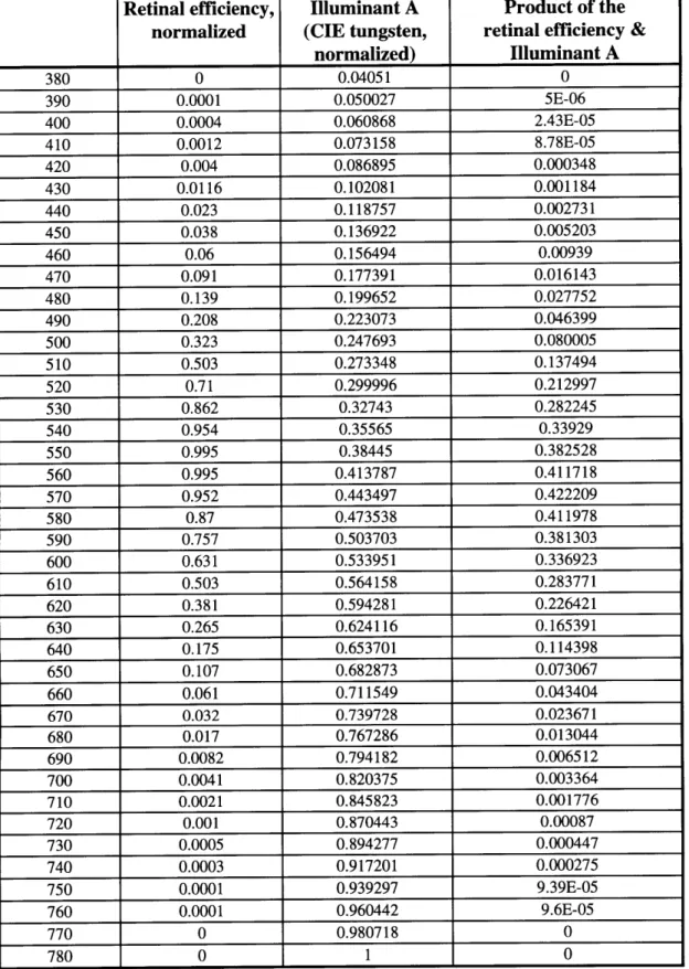
The relative intensities of the wavelengths have been normalized in Table 1.1 below. Each Illuminant A normalized value may be multiplied by the values for the corresponding wavelengths from the spectral luminous efficiency and diffraction efficiency curves. The resulting product of the corresponding Illuminant A and retinal efficiency data are listed in the rightmost column and represent what fraction of the light of that wavelength is delivered from the tungsten source to the hologram, and from the hologram to the eye, neglecting diffraction efficiencies.

(43)

Retinal efficiency, Illuminant A Product of the normalized (CIE tungsten, retinal efficiency &

normalized) Illuminant A 380 0 0.04051 0 390 0.0001 0.050027 5E-06 400 0.0004 0.060868 2.43E-05 410 0.0012 0.073158 8.78E-05 420 0.004 0.086895 0.000348 430 0.0116 0.102081 0.001184 440 0.023 0.118757 0.002731 450 0.038 0.136922 0.005203 460 0.06 0.156494 0.00939 470 0.091 0.177391 0.016143 480 0.139 0.199652 0.027752 490 0.208 0.223073 0.046399 500 0.323 0.247693 0.080005 510 0.503 0.273348 0.137494 520 0.71 0.299996 0.212997 530 0.862 0.32743 0.282245 540 0.954 0.35565 0.33929 550 0.995 0.38445 0.382528 560 0.995 0.413787 0.411718 570 0.952 0.443497 0.422209 580 0.87 0.473538 0.411978 590 0.757 0.503703 0.381303 600 0.631 0.533951 0.336923 610 0.503 0.564158 0.283771 620 0.381 0.594281 0.226421 630 0.265 0.624116 0.165391 640 0.175 0.653701 0.114398 650 0.107 0.682873 0.073067 660 0.061 0.711549 0.043404 670 0.032 0.739728 0.023671 680 0.017 0.767286 0.013044 690 0.0082 0.794182 0.006512 700 0.0041 0.820375 0.003364 710 0.0021 0.845823 0.001776 720 0.001 0.870443 0.00087 730 0.0005 0.894277 0.000447 740 0.0003 0.917201 0.000275 750 0.0001 0.939297 9.39E-05 760 0.0001 0.960442 9.6E-05 770 0 0.980718 0 780 0 1 0

Table 1.1: Data from the spectral luminous efficiency (Wyszecki and Stiles 1936) and Illuminant A relative intensity (MIT 1936) curves, and their corresponding products

(44)

Superposition of the two spectral component intensity filters: the retina and the illumination source

1 2 3 4 5 6 7 8 9 10 11 12 13 14 15 16 17 18 19 20 21 22 23 24 25 26 27 28 29 30 31 32 33 34 35 36 37 38 39 40 41

Wavelength (380-780nm)

Figure 1.22: Intensity filters: the retina and illuminant 1.11 Resolution of color-blurred reflection holographic images

The data used to make Figure 1.22 could have been multiplied by their

corresponding diffraction efficiency values for a complete determination of the relative intensities of the spectral components. However, the above analysis is only reasonable for application to transmission holograms with a wide spectral bandwidth (on the order of 200 to 300 nm), and is more extensive than it needs to be for thicker, reflection

holograms having a narrow spectral band (of about 20 to 30 nm).

For a narrow segment of the visual spectrum, the spectral luminous efficiency and relative illumination intensity curves are approximately linear and of small slope for the illumination source that was chosen. The diffraction efficiency curve, on the other hand, is very narrow about the central wavelength, and therefore of very steep slope. We will therefore consider the retinal and illuminant distributions to have a negligible effect on the perceived size of blurred image points. Instead, we will consider the perceived size to be wholly dependent on the diffraction efficiency distribution. First, we will define the resolvability of two blurred images, and then we will define the perceived size of a single blurred image point.

To define the resolvability of two blurred images, we will overlap the intensity distributions of two very closely situated images (as in section 1.7). A correspondence exists between distance from the center of a blurred image and playout wavelength, so the

(45)

spectral intensity distribution will enable us to determine the size of the image above a specified cutoff intensity. The distance from the center to the "boundary" of a blurred image is simply the length along the blur from the focused wavelength of highest diffraction efficiency to the focused wavelengths of some cutoff diffraction efficiency. We will define the minimum resolvable distance between two images as half of the distribution width at 50 percent intensity, the point on the Gaussian profile without curvature (Figure 1.23). We will further define the absolute bandwidth, AX, as those wavelengths contributing 95 percent of the intensity, from Equation (1.2):

Equation (1.3): I(r =-

±

095, with ra equal to half the absolute image size

Io e3

For a 50 percent spectral intensity cutoff, the minimum resolvable distance may be calculated from the absolute size of the blurred image, using the total calculated bandwidth.

minimum resolvable distance

50% intensity

- I(r) = 0.5 mrin

Figure 1.23: Just resolvable points defined by the diffraction efficiency curve. Here are two overlapping blurred images. As in Figure 1.18, the lines merely ascribe areas of the blurred image to points on corresponding intensity curves.

First, the bandwidth of the hologram may be defined using Equation (1.4)

(Syms1990, 7)14:

AX = cot(Oill), where A is the fringe spacing, A is the illumination wavelength, t2

t2 is the thickness of the grating, and Oill is the illumination angle.

14

Leith (1992) uses a completely different method for deriving the bandwidth, and defines the bandwidth

to equal the illumination wavelength divided by the number of fringes, N:

A A_-A

AA ~ -, Ths is equivalent to Sym's for the conformal (untilted) fringe case with ill= 45 degrees.

N t2

(46)

For most of the thesis, we will use a geometry with Oill = 450, and X = 514.5 nm.

For t2 = lOm:

From Benton (1994, 1996), we have Equation (1.5): A 2 out-

o

ill

2. i smil

-2 Therefore, AX = 34.59 nm.

The extreme wavelengths of this bandwidth may then be used in the calculations of Chapter 2 as the extreme raytracing wavelengths. For consistency, however, we will assume from this point forward a bandwidth of 20 nm for the different recording mediums we will be using.

Now we will calculate a "resolution factor," R, to determine the minimum resolvable distance between two points from the absolute blurred image height, hblur

(Chapter 2):

Mimimum resolvable distance = absolute image size x resolution factor (R), rso%

Equation (1.6): R =

rAA

- w21n(0.5)

From Equation (1.2): r5o% = 2 = 0.5887w,

and beam width w = 2r, 2, 0.8165rA

InL1 e 3 Therefore, R = 0.4807

An ideal quantity to which resulting minimum resolvable distance calculations may be compared may be obtained from Equation (1.2), Rayleigh's criterion:

1.22A

o = d . With a pupil diameter d=2.5mm and wavelength X=514.5 nm, the ideal

d

theoretical resolution is then 2.51 X 10-4 radians, about 5.2 arc seconds.

hblurmin x 0.4807

With a mimimum resolvable angle of 2.51 x 10- = ,

Deye

the minimum absolute blur height, hblurmin, is equal to 0.261 mm at a viewing distance

of 500 mm, or about 1.8 arc minutes.

For the rest of the thesis, we will be concerned primarily with determining the extent of the blur in holographic images, not with their resolution. Therefore, we need to perform a similar calculation as Equation (1.6) to find the perceived blur size.

(47)

1.12 Factor for perceived blur size

The perceived size of a blurred image is the absolute blurred image size, hblur (Chapter 2), multiplied by some perceived blur size factor, B. We will estimate this perceived blur size factor to be the ratio of the perceived height, hperceivedblur to the total height, hblur. Just as the total width of the gaussian distribution was marked by a cutoff intensity that also determined the boundary of the blurred image point, the distance

from the center to the perceived boundary of a blurred image is the radial distance from the center to a perceived cutoff intensity. As the beam width, defined above in section 1.9, contains 86.5 percent of the beam power, we will define our perceived bandwidth as the wavelengths playing out within the beam width. Now we are prepared to define a the perceived blur factor, B:

Perceived image size = absolute image size x perceived blur factor (B), w

Equation (1.7): R =

-From Equation (1.2), beam width w = -2, =0.8165rA

r1

In e 3 Therefore, B = 0.8165 1/e2 = 86.5% 1/e3= 95%

Figure 1.24: Perceived blur factor, B=0.8165

(48)

This perceived blur factor should be a reasonable approximation, considering the multiple sources of contrast degradation and noise mentioned above in section 1.7. In the next chapter, we will derive the absolute blur extent in terms of height, as well as angle subtended from the eye. The perceived blur factor may be applied to this absolute blur extent as an estimate of the perceived extent of a blurred image.

(49)

Chapter 2 Trigonometric derivation of a single-plane blur equation

In the previous chapter, we first looked at color blur from a qualitative standpoint, and applied successive intensity filters to determine the apparent size of a blurred image point as perceived by an observer. We found that we could define the extent of the perceived blur as well as resolution of blurred image points by simply approximating the diffraction efficiency of the recording material as a normal distribution about a mean wavelength, and defining the wavelengths at two standard deviations as the cutoff perceived wavelengths. In this chapter, we will take a more mathematical approach to define the absolute extent of this blur. We will then experimentally test the results with

spectrophotometer measurements. Finally, we will apply last chapter's perceived blur factor to the forthcoming derived blur equation.

The trigonometric derivation below gives us a formula for determining hologram color and source-size blur. We will compare the resulting formula with

Benton's blur equations. A vector blur equation is derived in Appendix 2, and reduces to the trigonometric form developed here.

2.1 Derivation of a color blur equation

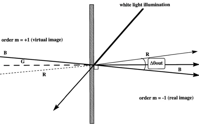
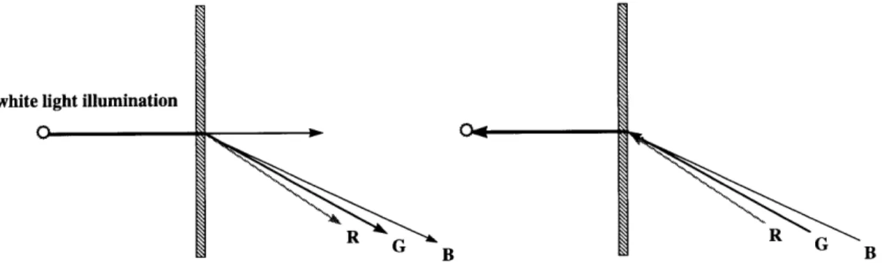
Figure 2.1 will provide us with the physical model we will be using in the derivation and future discussions. Spectral components of the illuminant reconstructing displaced images produce the blur. These components diffract at the hologram and create a "dispersed focus" at the pupil of the eye:

white light illumination

order m = +1 (virtual image)

R B

B

R

order m = -1 (real image)

Figure 2.1: Spectral components from different points on the hologram contributing to blur