HAL Id: hal-00317478
https://hal.archives-ouvertes.fr/hal-00317478
Submitted on 14 Jul 2004
HAL is a multi-disciplinary open access
archive for the deposit and dissemination of
sci-entific research documents, whether they are
pub-lished or not. The documents may come from
teaching and research institutions in France or
abroad, or from public or private research centers.
L’archive ouverte pluridisciplinaire HAL, est
destinée au dépôt et à la diffusion de documents
scientifiques de niveau recherche, publiés ou non,
émanant des établissements d’enseignement et de
recherche français ou étrangers, des laboratoires
publics ou privés.
Statistical behavior of foreshock Langmuir waves
observed by the Cluster wideband data plasma wave
receiver
K. Sigsbee, C. A. Kletzing, D. A. Gurnett, J. S. Pickett, A. Balogh, E. Lucek
To cite this version:
K. Sigsbee, C. A. Kletzing, D. A. Gurnett, J. S. Pickett, A. Balogh, et al.. Statistical behavior of
foreshock Langmuir waves observed by the Cluster wideband data plasma wave receiver. Annales
Geophysicae, European Geosciences Union, 2004, 22 (7), pp.2337-2344. �hal-00317478�
SRef-ID: 1432-0576/ag/2004-22-2337 © European Geosciences Union 2004
Annales
Geophysicae
Statistical behavior of foreshock Langmuir waves observed by the
Cluster wideband data plasma wave receiver
K. Sigsbee1, C. A. Kletzing1, D. A. Gurnett1, J. S. Pickett1, A. Balogh2, and E. Lucek2
1Department of Physics and Astronomy, 203 Van Allen Hall, University of Iowa, Iowa City, IA 52242, USA
2Space and Atmospheric Physics Group, The Blackett Laboratory, Imperial College, Prince Consort Road, London, SW7
2BW, UK
Received: 1 October 2003 – Revised: 8 June 2004 – Accepted: 11 June 2004 – Published: 14 July 2004 Part of Special Issue “Spatio-temporal analysis and multipoint measurements in space”
Abstract. We present the statistics of Langmuir wave
ampli-tudes in the Earth’s foreshock using Cluster Wideband Data (WBD) Plasma Wave Receiver electric field waveforms from spacecraft 2, 3 and 4 on 26 March 2002. The largest am-plitude Langmuir waves were observed by Cluster near the boundary between the foreshock and solar wind, in agree-ment with earlier studies. The characteristics of the waves were similar for all three spacecraft, suggesting that vari-ations in foreshock structure must occur on scales greater than the 50–100 km spacecraft separations. The electric field amplitude probability distributions constructed using wave-forms from the Cluster WBD Plasma Wave Receiver gener-ally followed the log-normal statistics predicted by stochas-tic growth theory for the event studied. Comparison with WBD receiver data from 17 February 2002, when space-craft 4 was set in a special manual gain mode, suggests non-optimal auto-ranging of the instrument may have had some influence on the statistics.
Key words. Magnetospheric physics (plasma waves and
in-stabilities; solar wind-magnetosphere interactions) – Inter-planetary physics (Inter-planetary bow shocks)
1 Introduction
The foreshock is a region upstream of the Earth’s bow shock that is magnetically connected to the bow shock. Within this region, electrons that are reflected and accelerated at the bow shock are convected downstream by the v×B electric field in the solar wind. The processes occurring near the shock produce electron beams and result in a bump-on-tail electron distribution function (Fitzenreiter et al., 1984). The Lang-muir waves observed in the Earth’s foreshock are thought to be generated by instabilities due to the bump-on-tail charac-ter of the electron beams in this region. The study performed by Filbert and Kellogg (1979) using IMP 6 data showed that
Correspondence to: K. Sigsbee
(kms@beta.physics.uiowa.edu)
the wave amplitudes were largest on magnetic field lines that were tangent to the bow shock. Using data from ISEE 1, Etcheto and Faucheux (1984) found that the maximum am-plitudes of the Langmuir waves were a few millivolts per me-ter at the edge of the foreshock and only a few tens to a few hundreds of microvolts per meter inside the foreshock. Dur-ing a time period when the solar wind magnetic field was unusually constant, Cairns et al. (1997) used ISEE 1 plasma wave data to show that there is a slight offset of the high wave amplitude region from the boundary of the foreshock. Cairns et al. also showed that the high field region is rel-atively narrow and that the field amplitudes fall off rather slowly at large distances from the foreshock. Other studies using ISEE 1 and Wind data (e.g. Bale et al., 1997; Cairns and Robinson, 1997) have examined the statistical proper-ties of the Langmuir wave amplitudes in order to identify various processes that may operate in the foreshock, such as Langmuir wave collapse (Zakharov, 1972), electrostatic decay (Robinson and Cairns, 1995; Bale et al., 2000), and stochastic growth (Robinson, 1995).
The multiple spacecraft nature of the Cluster mission al-lows us to investigate the behavior of Langmuir waves in the foreshock in ways that were not possible with earlier data sets. With Cluster, it is possible to compare near in-stantaneous Langmuir wave amplitudes at different posi-tions within the foreshock and examine moposi-tions of the fore-shock boundary. Another important feature of the Cluster data set from the Earth’s foreshock is that the WBD Plasma Wave Receiver provides electric field waveforms in this re-gion. Earlier studies of Langmuir waves in the Earth’s fore-shock conducted using data from ISEE (e.g. Greenstadt et al., 1995; Cairns et al., 1997), Geotail (Kasaba et al., 2000), and other spacecraft (e.g. Onsager et al., 1989) relied upon spectral density measurements, which can underestimate the wave amplitudes due to temporal and spectral averaging (see Robinson et al., 1993). The only known exceptions to this are the foreshock studies conducted using waveforms from the Wind spacecraft (e.g. Bale et al., 1997, 2000). In this paper, we present a study of Langmuir waves in the foreshock using
2338 K. Sigsbee et al.: Statistical behavior of Langmuir waves electric field waveforms from the Cluster WBD Plasma Wave
Receivers on spacecraft 2, 3 and 4 on 26 March 2002. This day was selected because there were relatively steady solar wind conditions during most of the time period that Clus-ter was located in the foreshock. The data from 26 March 2002 will be compared to results from the WBD receivers on Cluster spacecraft 3 and 4 for 17 February 2002 presented in Sigsbee et al. (2004).
2 Instrumentation
During the passes through the foreshock reported here, the WBD Plasma Wave Receiver was set in 77 kHz mode. For this bandwidth setting, the instrument obtains two back-to-back electric field waveform captures of approximately 5 ms each every 69.5 ms. The gain of the receiver can be set to amplifications between 0 and 75 dB in 5 dB increments. The peak amplitude range is 2.6×10⁻⁵mV/m to 36.9 mV/m or
123 dB, but the dynamic range in each gain state is 48 dB, corresponding to 8-bit digitization of the waveforms. The gain control can be set in either a fixed-gain mode or an auto-ranging mode. In fixed-gain mode, the gain can be set to any of the 16 levels between 0 and 75 dB. In the auto-ranging mode, the WBD receiver gain state is adjusted to keep the measured average amplitude within the range of the digitizer at the rate determined by gain update clock. For the full de-tails of the instrument and its operating modes, see Gurnett et al. (1997).
Because the amplitudes of Langmuir waves in the Earth’s foreshock can change on time scales of 1 ms or less, the 0.1 s time period of the Digital Wave Processor (DWP) (Wool-liscroft et al., 1997) gain update clock results in occasional clipping of the waveform peaks when the wave amplitudes exceed the maximum range for a particular gain state. On 17 February 2002, the WBD receiver on spacecraft 4 was operated with the gain manually set to 0 dB. This allowed us to consistently observe waveforms with amplitudes at the maximum range of the instrument (36.9 mV/m) without clipping of the peaks due to non-optimal auto-ranging and to investigate the effects of the automatic gain control on the waveform statistics. Setting the gain manually to 0 dB means that we can observe the large amplitude waves with-out clipping, but will miss low amplitude waves which fall below the minimum amplitude threshold for this gain state at 1.0 mV/m. The calibrated amplitudes increase linearly with the raw values, so waveforms with peak amplitudes less than 10.5 dB above the zero-level are not well-defined and resem-ble square waves. Waveforms with amplitudes in the lowest 10.5 dB of the 48 dB range for each gain state were ignored.
For Langmuir waves, the wave vector k is parallel to the background magnetic field. Because the WBD receiver an-tenna is located in the spin plane of the Cluster spacecraft, measurements near the plasma frequency in the foreshock can exhibit an amplitude modulation with a period of half the spacecraft spin period (4 s) due to the changing antenna ori-entation with respect to the background magnetic field. Some
studies of Langmuir waves in the foreshock have shown that while the most intense electric fields have wave vectors close to the magnetic field direction, the angular distribution of the largest amplitude waves can be very broad (Bale et al., 2000). However, during the time periods we have studied using Cluster data, the modulation of the wave amplitudes was distinct and well-correlated with the orientation of the antenna with respect to the magnetic field. In our study of Langmuir waves in the Earth’s foreshock, we multiplied the waveform amplitudes by the correction factor of 1/ cos θ , where θ is the angle between the antenna and the magnetic field. Data taken from 78◦≤θ ≤101◦were rejected because the amplitude correction factor becomes very large for an-gles close to 90◦. Applying the antenna angle correction to the waveform amplitudes increases the maximum amplitude that can be measured from 36.9 mV/m to 184.5 mV/m.
3 Foreshock coordinate system
Magnetic field data from the Cluster FGM experiment (Balogh et al., 1997) at 4 s resolution and a simple model bow shock were used to determine the position of the fore-shock boundary, which is defined by the location where the solar wind magnetic field is tangent to the bow shock. To determine the positions of the Cluster spacecraft within the Earth’s foreshock, we used the foreshock coordinate calcu-lation that was first described by Filbert and Kellogg (1979), and later modified by Fitzenreiter et al. (1990) and Cairns et al. (1997). For the complete mathematical description of this coordinate system, please refer to these papers. To simplify calculation of the magnetic field tangent point, we followed the procedure of Cairns et al. (1997) and rotated the positions and magnetic field about the x GSE axis into a new coordi-nate system where the magnetic field was completely in the x-y plane. Filbert and Kellogg (1979) used a paraboloid in GSE coordinates to represent the bow shock
x = as−bs(y2+z2), (1)
where as is the shock standoff distance from the Earth, and
bs determines the perpendicular scale of the shock. We took
nominal values of as=13.7 RE and bs=0.0223 RE−1 from
Cairns et al. (1997) and scaled as and bs to move the model
bow shock in and out with changes in the solar wind dynamic pressure. Solar wind parameters from the ACE spacecraft, propagated to Cluster’s location, were used to determine the appropriate scaling factors. After the point where the solar wind magnetic field is tangent to the model bow shock given by Eq. (1) has been found, we can express the spacecraft locations relative to the foreshock boundary.
Figure 1 illustrates the foreshock coordinate system for Cluster spacecraft 3 on 26 March 2002 at 01:39:58 UT. Be-fore calculating the location of the magnetic tangent point as described above, a rotation about the z GSE axis was ap-plied to the Cluster spacecraft positions and magnetic field data to account for the ∼4◦aberration of the magnetosphere symmetry axis due to the Earth’s orbital motion through the
Foreshock Position 2002-03-26 01:39:58
20
10
0
-10
-20
Rotated X GSE (RE)
-20
-10
0
10
20
RotatedYGSE(RE)
B
n
R
D
f Cluster SC 3 ( ) B Field Tangent Point ( ) B = (1.28, 11.77, 0.00) nT P = 4.32 nPaFig. 1. Illustration of the foreshock coordinate system for Cluster spacecraft 3 on 26 March 2002 at 01:39:58 UT.
interplanetary medium. Solar wind parameters from ACE, propagated to Cluster’s location, were used to calculate the actual aberration angle. In Fig. 1, the coordinate R gives the distance from the tangent point to the spacecraft parallel to the solar wind magnetic field. The parameter Df gives the distance from the spacecraft to the tangent field line in the x GSE direction, or in our case, the distance from the space-craft to the tangent field line along an axis ∼4◦from the x GSE direction when the aberration angle is taken into ac-count. The parameter Df used in this paper and by Cairns et al. (1997) is the same as the parameter DI F F used by Filbert and Kellogg (1979). In this model for the spacecraft location in the foreshock, changes in the parameters R and Df are due to a combination of the spacecraft motion and changes in the direction of the magnetic field, resulting in movement of the tangent point location. When the time-varying solar wind dynamic pressure is used to scale the bow shock model pa-rameters asand bs, changes in the shock location also affect
the foreshock coordinates R and Df.
4 Dependence of Langmuir wave amplitudes on fore-shock position
From 01:30:30 to 01:51:29 UT on 26 March 2002, the Clus-ter FGM experiment measured a fairly steady magnetic field of about 10 nT, dominated by large, northward Bz
compo-nent. When propagation effects are taken into account, ACE upstream magnetic field data show similar behavior. The x GSE component of the solar wind velocity measured by ACE was typically about −430 km/s and the density was near 14 cm−3. The WBD receivers on spacecraft 2, 3, and 4 observed intense waves near the plasma frequency (30–
Sampling Intervals and Peak Values
2.2470 2.2480 2.2490 2.2500 Time (seconds from 2002-03-26 01:51:25) -1.0 -0.5 0.0 0.5 1.0 SC3 E Field (mV/m)
Fig. 2. An example of a typical WBD electric field waveform from 26 March 2002. The vertical lines divide the waveform into 10 seg-ments, which were used to determine the peak electric field values for Figs. 3 and 4. The asterisks mark the peak electric field value in each segment. The amplitudes in this figure have not been corrected for the antenna angle to the magnetic field.
40 kHz) while Cluster was located in the foreshock from 01:30:30 to 01:51:29 UT. Around 01:51:29 UT, fluctuations in By with amplitudes greater than 5 nT and fluctuations
in Bz of ∼2–4 nT were observed which caused the
fore-shock boundary to move earthward of all three spacecraft from approximately 01:51:29–01:51:43 UT and 01:51:53– 01:52:07 UT. During these intervals, the Cluster spacecraft were located in the solar wind. The final entry into the solar wind during the time period studied in this paper occurred at 01:52:46 UT. The dynamic pressure measured by ACE was steady at ∼4.7 nPa between 01:51:29–01:52:46 UT, so the motion of the foreshock boundary during this time pe-riod was due to magnetic field fluctuations. Based upon the WBD receiver spectrograms, the spacecraft moved in and out of the foreshock within less than 1 s of each other during each of the five foreshock boundary crossings from 01:51:29 to 01:52:46 UT. The Cluster spacecraft were separated by only 50 to 100 km, so this implies that the boundary of the fore-shock moved over the spacecraft at speeds greater than 50– 100 km/s.
Figure 2 shows a typical WBD electric field waveform from 26 March 2002 and illustrates how we selected the elec-tric field values for our study. The amplitudes in the Fig. 2 waveform have not been corrected for the angle between the antenna and the magnetic field. As shown by Fig. 2, the Langmuir wave amplitudes can vary considerably on time scales of less than 1 ms. The peak electric field values used to examine the dependence of the amplitudes on position and to construct probability distributions in Sect. 5 were obtained by dividing each waveform into ten 0.5 ms segments, taking the absolute value of the electric field, and determining the maximum value in each segment. The vertical lines in Fig. 2 show the boundaries of the 0.5 ms segments and the asterisks mark the peak value in each segment. Segments containing
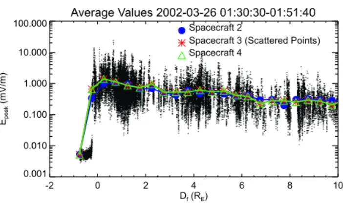
2340 K. Sigsbee et al.: Statistical behavior of Langmuir waves Average Values 2002-03-26 01:30:30-01:51:40 -2 0 2 4 6 8 10 Df(RE) 0.001 0.010 0.100 1.000 10.000 100.000 Epeak (mV/m) Spacecraft 2
Spacecraft 3 (Scattered Points) Spacecraft 4
Fig. 3. Dependence of the WBD receiver electric field amplitudes
on Dffor 26 March 2002 between 01:30:30–01:51:40 UT. The
scat-tered points represent the maximum electric fields in 0.5 ms win-dows of each 5-ms waveform snapshot for spacecraft 3, and the red
line represents the average electric field amplitudes in 0.5 RE bins
of the Df coordinate for spacecraft 3. The blue and green lines
rep-resent the average amplitudes for spacecraft 2 and 4.
clipped data and segments with maximum amplitudes below our minimum amplitude threshold were discarded because their amplitudes could not be accurately determined.
Figure 3 shows the peak Langmuir wave amplitudes as a function of the foreshock coordinate Df on 26 March 2002 for the time period 01:30:30–01:51:40 UT. The scattered points are the peak electric field amplitudes from spacecraft 3, determined using the method described in the preceding paragraph. The amplitudes used in Fig. 3 have been cor-rected for the angle between the WBD antenna and the mag-netic field as described in Sect. 2. The red line and points marked with asterisks represent the average values of the electric field for spacecraft 3 in 0.5 REwide bins of Df. The green and blue lines represent the average electric field val-ues from spacecraft 2 and 4, respectively. Df=0 marks the model location of the foreshock boundary. The group of points clustered between Df∼−1.0 to 0.0 RE and E∼0.003
to 0.007 mV/m represent thermal noise (Meyer-Vernet, 1979; Cairns et al., 2000) observed when Cluster was located in the solar wind from 01:51:29–01:51:40 UT. As the thermal noise level does not vary with the orientation of the antenna to the magnetic field, the amplitude correction was not applied to these points.
The sharp rise in the Langmuir wave amplitudes near
Df=−0.2 RE indicates the actual position of the foreshock
boundary determined by the data. Due to the small sep-arations of the Cluster spacecraft, the dependence of the amplitudes on Df for spacecraft 2, 3 and 4 on 26 March 2002, shown in Fig. 3, are nearly identical. The near-simultaneous observations of waves with similar ampli-tudes implies that the foreshock structure is fairly uni-form on scales of 50 to 100 km, and supports earlier sta-tistical studies showing that far away from the bound-ary significant changes in the average wave amplitudes in the foreshock occur on scales greater than ∼0.5–1.0 RE
(Greenstadt et al., 1995; Kasaba et al., 2000).
In Fig. 3, the largest average field values, about 1–2 mV/m for all three spacecraft, were found in the 0.0<Df<0.5 RE
bin. The scattered points for spacecraft 3 shown in Fig. 3 indicate that waves with amplitudes from 0.1 mV/m up to 20 mV/m were observed in this region. The location of the largest wave amplitudes in Fig. 3 agrees reason-ably well with the work of Cairns et al. (1997) which also showed that the largest amplitudes were observed near
Df∼0.5 RE. However, in the data presented by Cairns et
al. the wave amplitudes increased slowly with decreasing
Df for 1.0<Df<6.0 RE but increased by more than a factor
of 10 between 0.5<Df<1.0 RE, creating a distinct high-field
region about 1.0 RE wide. In the 17 February 2002 case,
studied by Sigsbee et al. (2004), the data from the WBD re-ceiver on spacecraft 3 also show a clear boundary between the foreshock and solar wind, and a distinct high-field region of about 1 RE wide where the amplitudes increase rapidly.
The data shown in Fig. 3 indicate that the Langmuir wave amplitudes increased gradually with decreasing Df through-out the foreshock and that there was not a distinct high-field region near the foreshock boundary for the time period stud-ied on 26 March 2002.
Cairns et al. (1997) estimated that there was ∼±0.4 RE
uncertainty in Df due to uncertainties in the values of the
as and bs parameters in the shock model. The offset of
the rise in wave amplitudes near the foreshock boundary in Fig. 3 implies that the error in Df is only about 0.2 REfor the
01:30:30–01:51:40 UT time period. The fact that no thermal noise points were observed for Df>0 RE also suggests that
the bow shock model we used is generally reasonable and gives an accurate calculation of the position in the foreshock when the solar wind magnetic field is steady. The location of the actual foreshock boundary in Fig. 3 is quite clear and is the same for all three spacecraft, which implies that the positions of the spacecraft relative to the foreshock boundary are well-defined for the 01:30:30–01:51:40 UT time period, even if there is a small offset in the absolute location of the boundary determined by the electric field amplitudes. How-ever, the error in Df was considerably larger when the fore-shock boundary was in motion from 01:51:43–01:52:46 UT. More than 85% of the values greater than 0.01 mV/m mea-sured by spacecraft 3 between 01:51:43 and 01:52:46 UT were placed at Df<0 RE, even though these waves were
ob-served in the foreshock. Simulations have shown that when the solar wind magnetic field is turbulent, it is possible for a spacecraft to be magnetically connected to the bow shock, even when it is upstream of the nominal foreshock bound-ary and that the spread in the boundbound-ary location can be as much as 1 RE (Zimbardo and Veltri, 1996). This is a likely
explanation why the position calculation was not accurate for 01:51:43 to 01:52:46 UT.
Figure 3 shows that for 2.0<Df<10.0 RE, the average
corrected amplitude of the waves observed in the fore-shock by the WBD receiver on 26 March 2002 ranged from 0.3 mV/m to 0.5 mV/m. In the 17 February 2002 data stud-ied by Sigsbee et al. (2004), the average corrected amplitude for this range of Df values was usually between 0.7 mV/m
to 0.8 mV/m, with amplitudes varying from 0.1 mV/m up to 4.0 mV/m. The largest amplitude waves observed on 17 February 2002 extended to the maximum range of the WBD receiver (36.9 mV/m) and had corrected peak amplitudes up to 100 mV/m near the foreshock boundary. However, the largest corrected amplitudes for 26 March 2002, shown in Fig. 3, were only 20.0 mV/m. Waves with corrected am-plitudes up to 60 mV/m were observed from 01:51:43 to 01:52:46 UT when the foreshock boundary was in rapid mo-tion due to fluctuamo-tions of the magnetic field, but were not included in Fig. 3 as the error in Df was too large due to the boundary motions. On 17 February 2002, the background magnetic field was more closely aligned with the WBD an-tennas than it was on 26 March 2002. The less favorable ori-entation of the spacecraft with respect to the magnetic field on 26 March 2002 is the most likely reason why the ampli-tudes of the waves observed on this day were smaller than those observed on 17 February 2002. However, other factors may have also contributed to the difference in the wave am-plitudes. For the time period of interest on 26 March 2002, the average Alfv´en Mach number calculated using ACE data was 6.6. For the time period studied on 17 February 2002, the average Alfv´en Mach number was 5.7. In a study of elec-trostatic waves near the Earth’s bow shock using AMPTE IRM data, Onsager et al. (1989) found that the wave ampli-tudes decreased with increasing Alfv´en Mach number. Our observations appear to be consistent with the results of this study.
5 Amplitude probability distributions
The statistics of the electric field waveform amplitudes in the foreshock can also be used to examine possible growth mech-anisms for the Langmuir waves, such as stochastic growth theory. Stochastic growth theory considers the behavior of waves subject to a randomly varying growth rate (Robinson, 1995). Spatial inhomogeneities and time-varying perturba-tions in the plasma cause the appearance of regions of pos-itive and negative growth rate. Waves propagating through these regions grow at a rate that fluctuates randomly around the mean. According to Cairns and Robinson (1999, and references therein), the amplitude probability distribution is Gaussian in log E
P (log E) = (σ
√
2π )−1e−(log E−µ)2/2σ2, (2) where µ and σ are the average and standard deviation of log E. Using Wind TDS data, Bale et al. (1997) found that the amplitude probability distribution for Langmuir waves in the foreshock actually resembled a power law
P (log E)∝E−0.99. Cairns and Robinson (1997) found that the observed ISEE 1 electric field amplitude probability dis-tribution agreed with the stochastic growth theory predic-tion given by Eq. (2) for a constant spacecraft locapredic-tion rel-ative to the foreshock boundary. For periods with large variation in the spacecraft location, they found a power law
P (log E)∝E−0.8±0.3. This led Cairns and Robinson to
con-clude that the power law distribution of amplitudes was the result of the convolution of the actual amplitude probability distribution with the spacecraft motion.
To construct the probability distributions for the WBD re-ceiver data, we divided the full 123 dB amplitude range into 2.5 dB wide bins. Since the gain setting of the WBD Plasma Wave Receiver increases or decreases in 5 dB steps, choos-ing an amplitude bin width of 2.5 dB will allow the bins in the different gain states to exactly match in the overlapping portions of their amplitude ranges. We found the peak ampli-tudes, as described in Sect. 4, and then determined the per-centage of waveforms in each amplitude bin. We first con-structed amplitude probability distributions including elec-tric fields measured for all values of Df. To account for the fact that Cluster did not spend equal amounts of time at each position, we weighted every count in the electric field am-plitude bins by the number of points in the Df bin with the fewest points divided by the number of points in the Df bin where the measurement was taken. To investigate the possi-bility that the behavior of the waves may vary with position in the foreshock, we also constructed probability distributions using only measurements taken in 1 RE bins of Df for the range −1.0<Df<10.0 RE. No weighting factors were
ap-plied to the counts used to construct the probability distribu-tions in the 1 REbins of Df.
Figure 4a, b and c show the probability distributions from 26 March 2002 for the time period 01:30:30–01:51:40 UT, using weighted counts for all values of Df less than 10 RE
for spacecraft 2, 3 and 4, respectively. The dotted lines show the fits to the Gaussian function predicted by stochas-tic growth theory. The probability distributions are similar for all three spacecraft, as would be expected based upon the agreement of average waveform amplitudes for all three spacecraft shown in Fig. 3. The probability distributions for all values of Df from the three spacecraft fit reasonably well to a Gaussian over the entire amplitude range shown in Fig. 4. In contrast, the probability distribution for all values of Df from Cluster spacecraft 3 on 17 February 2002, discussed in Sigsbee et al. (2004), appeared to be Gaussian for amplitudes less than 1–2 mV/m but resembled a power law for larger am-plitudes.
Figure 4d shows the probability distributions from se-lected 1 RE bins in Df for spacecraft 4 for the time
pe-riod 01:30:30–01:51:40 UT on 26 March 2002 with fits to a Gaussian (dotted line). The probability distributions for the 0.0<Df<1.0 RE, 1.0<Df<2.0 RE, 2.0<Df<3.0 RE, and
3.0<Df<4.0 RE bins fit well to the prediction of
stochas-tic growth theory at all amplitudes, with reduced chi-squared values of 4.0, 6.8, 2.4, and 1.1, respectively. The probability distributions for the 1 REbins of Df fit better to a Gaussian than the probability distributions including all values of Df, which had reduced chi-squared values of 12.2 for spacecraft 2, 9.1 for spacecraft 3, and 8.6 for spacecraft 4. The probabil-ity distributions calculated in bins of Df for the 17 February 2002 case studied by Sigsbee et al. (2004) also appeared to be Gaussian at all distances to the foreshock boundary. When
2342 K. Sigsbee et al.: Statistical behavior of Langmuir waves 0.001 0.010 0.100 1.000 P(log E) SC 2 All Values of Df<10 RE Weighted Counts N = 35168 (a) 0.001 0.010 0.100 1.000 P(log E) SC 3 All Values of Df<10 RE Weighted Counts N = 34175 (b) 0.001 0.010 0.100 1.000 P(log E) SC 4 All Values of Df<10 RE Weighted Counts N = 35153 (c) 0.001 0.010 0.100 1.000 10.000 E (mV/m) 0.001 0.010 0.100 1.000 P(log E) SC 4 Selected Bins of Df 0.0<Df<1.0 N=7915 (d) 1.0<Df<2.0 N=7935 2.0<Df<3.0 N=1431 3.0<Df<4.0 N=2879
Fig. 4. Probability distributions for the electric field waveform am-plitudes observed by the Cluster WBD Plasma Wave Receiver on
26 March 2002. The probability distributions for all values of Df
using weighted counts for (a) spacecraft 2, (b) spacecraft 3, and (c) spacecraft 4. The dashed lines show the fit to the Gaussian function predicted by stochastic growth theory. (d) Probability distributions
from spacecraft 4 for selected 1 REbins in Df.
the data were organized into bins of Df, the probability dis-tributions for 26 March 2002 and for the 17 February 2002 case studied by Sigsbee et al. both show that the center of the probability distributions shifts gradually toward lower ampli-tudes as the spacecraft goes deeper into the foreshock, in a manner consistent with the average amplitudes for each bin. This is also consistent with the results of Filbert and Kellogg (1979) and Cairns and Robinson (1999).
In the 17 February 2002 data, it appeared that the power law tail on the probability distribution calculated using weighted counts from all values of Df was effectively the result of summing the distributions calculated in different
bins of position over Df. On 17 February 2002, the average corrected wave amplitudes increased by less than 0.1 mV/m per RE with decreasing Df deep inside the foreshock, but they increased by more than 5 mV/m per RE within 1.5 RE
of the foreshock boundary. Close to the foreshock bound-ary, corrected amplitudes reached values near 100 mV/m on 17 February 2002. Although the 17 February 2002 proba-bility distributions for each bin of Df values were Gaussian in form, the sudden increase in the center electric field am-plitude of the distributions close to the foreshock boundary caused their sum to have a power law tail at large ampli-tudes. The 17 February 2002 data clearly support the results of Boshuizen et al. (2001), which showed that spatially aver-aged probability distributions including measurements from a wide range of Df values will appear to be power laws.
The reason why the 26 March 2002 probability distribu-tions for all values of Df shown in Fig. 4 do not have a power law tail at large amplitudes can be understood by examining Fig. 3. The average corrected amplitudes in Fig. 3 increase steadily by about 0.1–0.2 mV/m per REright up to the
fore-shock boundary. Since the shift of the centers of the prob-ability distributions for individual bins of Df for 26 March 2002 was more constant throughout the foreshock, the total distribution for all values of Df still appears to be Gaussian.
6 Effects of non-optimal auto-ranging on statistics
Nearly every study of waves in the foreshock has relied upon data from an instrument that either has used some sort of au-tomatic ranging or auau-tomatic selection of waveform captures based upon amplitude. However, automatic ranging can in-troduce bias into the amplitude statistics. Figure 5 shows the percentages of waveforms in each gain state rejected due to clipping or because the peak amplitudes were below the min-imum amplitude threshold for spacecraft 3 for both 26 March 2002 and 17 February 2002. On 17 February 2002, a total of 18.2% of the waveforms were rejected. On 26 March 2002, 21.2% of the waveforms were rejected.
Figure 5a shows that on 17 February 2002 less than 40% of the waveforms in the 15 dB to 50 dB gain states were re-jected, and the 60 dB gain state was the only setting where more than 50% of the waveforms were rejected. Figure 5b shows that on 26 March 2002, less than 40% of the wave-forms were rejected in the 30 dB to 55 dB gain states, which is a considerably smaller portion of the amplitude range than on 17 February 2002. Also, Fig. 5b shows on 26 March 2002 that 50% or more of the waveforms were rejected in the 0 dB to 20 dB gain states and in the 65 dB to 75 dB gain states. Al-though the average wave amplitudes observed on 26 March 2002 appear to have been distinctly lower than on 17 Febru-ary 2002, elimination of waveforms due to non-optimal auto-ranging may help explain why there were so few waves ob-served with uncorrected amplitudes greater than 10 mV/m on 26 March 2002. In the 26 March 2002 data, 4.6% of the waveforms were rejected due to clipping, but only 4.3% were rejected due to clipping in the 17 February 2002 data. The
largest amplitude waves observed on 26 March 2002 were very bursty and transient in nature, and the 0.1 s gain up-date rate appeared to be much slower than the time scales on which the amplitudes of the waves changed. This probably resulted in the WBD receivers not always being set in the most appropriate gain state, as the automatic gain control at-tempted to compensate for the rapidly changing amplitudes, and can also explain why a larger percentage of waveforms were rejected on 26 March 2002 because they fell below the minimum amplitude threshold.
The effects of the automatic gain control may offer an ex-planation why the probability distributions sometimes vary from the expected shape. Manually setting the gain state is one way to deal with this problem, however, the probability distribution obtained will only be valid for a limited ampli-tude range. On 17 February 2002, the gain on spacecraft 4 was manually set to 0 dB. Only 0.03% of the waveforms ob-served by spacecraft 4 were excluded due to clipping, but more than 95% of the waveforms had to be rejected because they fell below the minimum amplitude threshold. The result was that the probability distributions constructed for space-craft 4 on 17 February 2002 by Sigsbee et al. (2004) were only valid for uncorrected amplitudes between 2.0 mV/m and 36.9 mV/m. The WBD receiver was designed with a great deal of overlap between the amplitude ranges for the various gain settings, so it may be possible to correct for the effects of non-optimal auto-ranging by comparing the results from different gain states for the same amplitude range. Studies are currently underway to do this comparison.
7 Conclusions
The Cluster WBD Plasma Wave Receiver observations on 26 March 2002 are consistent with earlier studies of Langmuir waves in the foreshock conducted using data from Wind and ISEE 1 (Bale et al., 1997; Cairns and Robinson, 1997). Typ-ical Langmuir wave electric field amplitudes in the Earth’s foreshock are on the order of a few mV/m or less, but waves with amplitudes greater than 10 mV/m are occasionally ob-served. The largest amplitude waves were observed near the boundary of the foreshock, consistent with earlier stud-ies. However, the waves observed on 26 March 2002 were generally lower in amplitude than the waves on 17 February 2002, discussed by Sigsbee et al. (2004), and the high-field region near the foreshock boundary was less distinct than on 17 February 2002. The behavior of the magnetic field and the higher Alfv´en Mach number on 26 March 2002 may explain these differences. The amplitude of the Langmuir waves fell off at a fairly steady rate with increasing distance from the foreshock boundary on 26 March 2002. This behavior is dif-ferent from the results of Sigsbee et al. (2004) and Cairns et al. (1997), which showed a sudden decrease close to the boundary, and a more gradual decrease far from the bound-ary. The dependence of the amplitudes on distance to the foreshock boundary was the same for Cluster spacecraft 2, 3, and 4 during the time period studied on 26 March 2002.
Total # of Waveforms = 896800 SC3 2002-02-17 09:13:19 to 2002-02-17 10:13:55 60 40 20 0 Gain (dB) 0 20 40 60 80 100 P ercentage of W a vef or ms Rejected 20% 40% # Below Threshold = 124119 # Clipped = 39194 Total # of Waveforms = 329079 SC3 2002-03-26 01:30:30 to 2003-03-26 01:52:46 60 40 20 0 Gain (dB) 0 20 40 60 80 100 P ercentage of W a vef or ms Rejected 20% 40% # Below Threshold = 54711 # Clipped = 15206 (a) (b)
Fig. 5. Histograms of the percentages of waveforms in each gain state rejected for (a) spacecraft 3 on 17 February 2002 and (b) spacecraft 3 on 26 March 2002. The solid black line indicates the total percentages of waveforms rejected in each gain state. The gray shaded area indicates the percentage of clipped waveforms and the line-filled area indicates the percentage of waveforms below the minimum amplitude threshold.
Comparison with the predictions of stochastic growth the-ory shows that the Langmuir wave observations for 26 March 2002 followed the log-normal statistics predicted by tic growth theory. Power law deviations from the stochas-tic growth theory prediction at large amplitudes have been well-documented (Bale et al., 1997; Cairns and Robinson, 1999; Sigsbee et al., 2004). These deviations generally occur when electric field amplitudes from a large range of distances from the foreshock boundary are included in the probability distribution. However, even when data from a large range of distances to the foreshock boundary were included in the 26 March 2002 probability distributions, they followed log-normal statistics. The behavior of the waves on 26 March 2002 may have been physically different from what has been observed in previous studies, but the errors in the Df cal-culation close to the foreshock boundary and the effects of non-optimal auto-ranging of the instrument could also have influenced the statistics.
2344 K. Sigsbee et al.: Statistical behavior of Langmuir waves Acknowledgements. We thank the ACE SWEPAM and MAG
In-strument Teams and the ACE Science Data Center for providing the ACE data. This work was supported by NASA/GSFC grant NAG5-9974.
Topical Editor T. Pulkkinen thanks S. D. Bale and another ref-eree for their help in evaluating this paper.
References
Bale, S. D., Burgess, D., Kellogg, P. J., Goetz, K., and Monson, S. J.: On the amplitude of intense Langmuir waves in the terrestrial electron foreshock, J. Geophys. Res., 102, 11 281–11 286, 1997. Bale, S. D., Larson, D. E., Lin, R. P., Kellogg, P. J., Goetz, K., and Monson, S. J.: On the beam speed and wavenumber of intense electron plasma waves near the foreshock edge, J. Geophys. Res., 105, 27 353–27 367, 2000.
Balogh, A., Dunlop, M. W., Cowley, S. W. H., Southwood, D. J., Thomlinson, J. G., Glassmeier, K. H., Musmann, G., Luhr, H., Buchert, S., Acuna, M. H., Fairfield, D. H., Slavin, J. A., Riedler, W., Schwingenschuh, K., and Kivelson, M. G.: The Cluster mag-netic field investigation, Space Sci. Rev., 79, 65–91, 1997. Boshuizen, C. R., Cairns, I. H., and Robinson, P. A.: Stochastic
growth theory of spatially-averaged distributions of Langmuir fields in Earth’s foreshock, Geophys. Res. Lett., 28, 3569–3572, 2001.
Cairns, I. H. and Robinson, P. A.: First test of stochastic growth theory for Langmuir waves in Earth’s foreshock, Geophys. Res. Lett., 24, 369–372, 1997.
Cairns, I. H. and Robinson, P. A.: Strong evidence for stochastic growth of Langmuir-like waves in Earth’s foreshock, Phys. Rev. Lett., 82, 3066–3069, 1999.
Cairns, I. H., Robinson, P. A., Anderson, R. R., and Strangeway, R. J.: Foreshock Langmuir waves for unusually constant solar wind conditions: Data and implications for foreshock structure, J. Geophys. Res., 102, 24 249–24 264, 1997.
Cairns, I. H., Robinson, P. A., and Anderson, R. R.: Thermal and driven stochastic growth of Langmuir waves in the solar wind and Earth’s foreshock, Geophys. Res. Lett., 27, 61–64, 2000. Etcheto, J. and Faucheux, M.: Detailed study of electron plasma
waves upstream of the Earth’s bow shock, J. Geophys. Res., 89, 6631–6653, 1984.
Filbert, P. C. and Kellogg, P. J.: Electrostatic noise at the plasma frequency beyond the Earth’s bow shock, J. Geophys. Res., 84, 1369–1381, 1979.
Fitzenreiter, R. J., Klimas, A. J., and Scudder, J. D.: Detection of bump-on-tail reduced electron velocity distributions at the electron foreshock boundary, Geophys. Res. Lett., 11, 496–499, 1984.
Fitzenreiter, R. J., Scudder, J. D., and Klimas, A. J.: Three-dimensional analytical model for the spatial variation of the fore-shock electron distribution function: Systematics and Compar-isons with ISEE observations, J. Geophys. Res., 95, 4155–4173, 1990.
Greenstadt, E. W., Crawford, G. K., Strangeway, R. J., Moses, S. L., and Coroniti, F. V.: Spatial distribution of electron plasma oscillations in the Earth’s foreshock at ISEE 3, J. Geophys. Res., 100, 19 933–19 939, 1995.
Gurnett, D. A., Huff, R. L., and Kirchner, D. L.: The Wide-Band Plasma Wave Investigation, Space Sci. Rev., 79, 195–208, 1997. Kasaba, Y., Matsumoto, H., Omura, Y., Anderson, R. R., Mukai, T., Saito, Y., Yamamoto, T., and Kokubun, S.: Statistical studies of plasma waves and backstreaming electrons in the terrestrial electron foreshock observed by Geotail, J. Geophys. Res., 105, 79–103, 2000.
Meyer-Vernet, N.: On natural noises detected by antennas in plas-mas, J. Geophys. Res., 84, 5373–5377, 1979.
Onsager, T. G., Holzworth, R. H., Koons, H. C., Bauer, O. H., Gur-nett, D. A., Anderson, R. R., L¨uhr, H., and Carlson, C. W.: High-frequency electrostatic waves near Earth’s bow shock, J. Geo-phys. Res., 94, 13 397–13 408, 1989.
Robinson, P. A.: Stochastic wave growth, Phys. Plasmas, 2, 1466– 1479, 1995.
Robinson, P. A. and Cairns, I. H.: Maximum Langmuir fields in planetary foreshocks determined from the electrostatic decay threshold, Geophys. Res. Lett., 22, 2657–2660, 1995.
Robinson, P. A., Cairns, I. H., and Gurnett, D. A.: Clumpy Lang-muir waves in type III radio sources: comparison of stochastic-growth theory with observations, Astrophys. J., 407, 790–800, 1993.
Sigsbee, K., Kletzing, C. A., Gurnett, D. A., Pickett, J. S., Balogh, A., and Lucek, E.: The dependence of Langmuir wave ampli-tudes on position in Earth’s foreshock, Geophys. Res. Lett., 31, L07805, doi:10.1029/2004GL019413, 2004.
Woolliscroft, L. J. C., Alleyne, H., Dunford, C. M., Sumner, A., Thompson, J. A., Walker, S. N., Yearby, K. H., Buckley, A., Chapman, S., and Gough, M. P.: The Digital Wave Processing Experiment on Cluster, Space Sci. Rev., 79, 209–231, 1997. Zakharov, V. E.: Collapse of Langmuir waves, Sov. Phys. JETP, 35,
908–914, 1972.
Zimbardo, G. and Veltri, P.: Spreading and intermittent structure of the upstream boundary of planetary magnetic foreshocks, Geo-phys. Res. Lett., 23, 793–796, 1996.