HAL Id: hal-00296781
https://hal.archives-ouvertes.fr/hal-00296781
Submitted on 11 Jul 2003
HAL is a multi-disciplinary open access
archive for the deposit and dissemination of
sci-entific research documents, whether they are
pub-lished or not. The documents may come from
teaching and research institutions in France or
abroad, or from public or private research centers.
L’archive ouverte pluridisciplinaire HAL, est
destinée au dépôt et à la diffusion de documents
scientifiques de niveau recherche, publiés ou non,
émanant des établissements d’enseignement et de
recherche français ou étrangers, des laboratoires
publics ou privés.
Space Gravity Spectroscopy - determination of the
Earth?s gravitational field by means of Newton
interpolated LEO ephemeris Case studies on dynamic
(CHAMP Rapid Science Orbit) and kinematic orbits
T. Reubelt, G. Austen, E. W. Grafarend
To cite this version:
T. Reubelt, G. Austen, E. W. Grafarend. Space Gravity Spectroscopy - determination of the Earth?s
gravitational field by means of Newton interpolated LEO ephemeris Case studies on dynamic (CHAMP
Rapid Science Orbit) and kinematic orbits. Advances in Geosciences, European Geosciences Union,
2003, 1, pp.127-135. �hal-00296781�
Advances in Geosciences (2003) 1: 127–135 c
European Geosciences Union 2003
Advances in
Geosciences
Space Gravity Spectroscopy - determination of the Earth’s
gravitational field by means of Newton interpolated LEO ephemeris
Case studies on dynamic (CHAMP Rapid Science Orbit) and
kinematic orbits
T. Reubelt, G. Austen, and E. W. Grafarend
Geodetic Institute, Stuttgart University, Geschwister-Scholl-Str. 24/D, D-70174 Stuttgart, Germany
Abstract. An algorithm for the (kinematic) orbit analysis
of a Low Earth Orbiting (LEO) GPS tracked satellite to de-termine the spherical harmonic coefficients of the terrestrial gravitational field is presented. A contribution to existing long wavelength gravity field models is expected since the kinematic orbit of a LEO satellite can nowadays be deter-mined with very high accuracy in the range of a few cen-timeters. To demonstrate the applicability of the proposed method, first results from the analysis of real CHAMP Rapid Science (dynamic) Orbits (RSO) and kinematic orbits are illustrated. In particular, we take advantage of Newton’s Law of Motion which balances the acceleration vector and the gradient of the gravitational potential with respect to an Inertial Frame of Reference (IRF). The satellite’s accelera-tion vector is determined by means of the second order func-tional of Newton’s Interpolation Formula from relative satel-lite ephemeris (baselines) with respect to the IRF. There-fore the satellite ephemeris, which are normally given in a Body fixed Frame of Reference (BRF) have to be trans-formed into the IRF. Subsequently the Newton interpolated accelerations have to be reduced for disturbing gravitational and non-gravitational accelerations in order to obtain the ac-celerations caused by the Earth’s gravitational field. For a first insight in real data processing these reductions have been neglected. The gradient of the gravitational potential, conventionally expressed in vector-valued spherical harmon-ics and given in a Body Fixed Frame of Reference, must be transformed from BRF to IRF by means of the polar motion matrix, the precession-nutation matrices and the Greenwich Siderial Time Angle (GAST). The resulting linear system of equations is solved by means of a least squares adjustment in terms of a Gauss-Markov model in order to estimate the spherical harmonics coefficients of the Earth’s gravitational field.
Key words. space gravity spectroscopy, spherical
harmon-ics series expansion, GPS tracked LEO satellites, kinematic Correspondence to: T. Reubelt
(reubelt@gis.uni-stuttgart.de)
orbit analysis, Newton interpolation
1 Reference frames
First, the beforehand mentioned transformation between the Inertial Reference Frame and the Body Fixed Reference Frame is considered for this contribution more an issue of the operational point of view (software development) since the underlying theoretical aspects are well known, eg. Mc-Carthy (1996). The resulting transformation matrix R(t ) contains the parameters of nutation, precession, polar motion and Greenwich siderial time. Corrections for the nutation model and the parameters for polar motion and Greenwich siderial time are delivered by the Bulletins of the Interna-tional Earth Rotation Service (IERS).
2 Representation of the Earth’s gravitational field – the spherical harmonics series expansion
For the description of the gravitational field of the Earth we use a spherical harmonics series expansion. Equation (1) defines this series expansion of the gravitational potential
U (λ, ϕ, r)as an infinite sum. In our approach the summa-tion is only executed to a maximum sensitivity degree L, constituted by the measurement principle of CHAMP. GM denotes the geocentric gravitational constant, R the mean ra-dius of the Earth, l and m degree and order of the spheri-cal harmonics series expansion and Pl,m∗ (sin ϕ) are Ferrer’s fully normalized associated Legendre functions. ul,m
iden-tify the unknown spherical harmonic coefficients which we aim to determine. These coefficients ul,mcan be divided into
coefficients cl,m (cosine term, m ≥ 0) and sl,m (sine term, m <0).
Ferrer’s fully normalized associated Legendre-functions
Pl,m∗ (sin ϕ) are obtained from the associated Legendre-functions Pl,m(sin ϕ) by normalisation according to Eq. (2).
as-128 T. Reubelt et al.: Space Gravity Spectroscopy
Table 1
spherical harmonics series expansion of the Earth’s gravity field
1 , , 0 , , cos( ) 0 GM R U( , , ) lim (sin ) sin( ) 0 R ( )! 2(2 1) (sin ) ; 0 ( )! (sin ) : 2 1 l L l l m l m L l m l l m l m l m m r u P m m r subject to
"Ferrer's fully normalized associated Legendre- functions" l m l P m l m P l P λ λ ϕ ϕ λ ϕ ϕ + + ∗ →∞ = =− ∗ ≥ = < − + ⋅ ≠ + = + ⋅
∑ ∑
,0(sin )ϕ ;m 0 = (1)
(2)
-3,0E-09 -2,0E-09 -1,0E-09 0,0E+00 1,0E-09 2,0E-09 3,0E-09 90 1090 2090 3090 4090 5090 time in [s] errors in m/s²Fig. 1. Interpolation errors of Newton interpolated accelerations
X for one simulated CHAMP revolution based on EGM96 up to
degree/order 50/50; sampling time 1t = 30 s; 9-point scheme; x-axis: time in [s]; y-x-axis: acceleration error in [m/s2]
sociated Legendre functions recurrence formulae are applied (Koop and Stelpstra, 1989; Belikov and Taybatarov, 1992).
3 Determination of accelerations by means of Newton interpolation
For the determination of accelerations from GPS tracked absolute ephemeris X(t) or baselines 1X(t ) we have cho-sen Newton’s interpolation formula for equidistant sampling points (Engeln-M¨ullges and Reutter, 1966). Based on the zero order functional, Eq. (3), we derive Newton’s second order interpolation formula in Eq. (7) which is computed by a product-sum of forward differences (Eq. 5) and the sec-ond order functional of Newton’s base polynomials (Eq. 8). Newton’s base polynomials (Eq. 6) contain the time differ-ence quotient q (Eq. 4) and are received via q over i. The forward differences are originally determined from absolute ephemeris (Eq. 5), but in our case the forward differences can be expressed in terms of relative ephemeris (baselines of ad-jacent positions, Eq. 9). Since adad-jacent ephemeris are highly correlated (and thus relative ephemeris can be determined a
lot more precise than absolute ones), an improvement of ac-curacy is realized.
For our purpose, the application of the 9-point scheme has turned out to provide the best approximation (Austen and Reubelt, 2000), and so the following computations and fig-ures are based upon the 9-point interpolation scheme.
In general a n-point interpolation scheme can be consid-ered as a mask, which allows the computation of accelera-tion vectors from sets of n satellite’s CoM (Center of Mass) position vectors. This mask is moved successively through the position time series generating an acceleration time se-ries, which has to be further corrected for disturbing acceler-ations caused by atmospheric drag, solar radiation pressure, third body effects, etc. Again the operational implementation is very laborious, for details one can consult Hartmann and Wenzel (1995), King-Hele (1987) and Wahr (1995). Due to the immense number of observations it is possible to proceed the mask in a non - overlapping way to avoid correlation for consecutive mask positions.
4 Performance analysis of Newton interpolation
4.1 Approximation error
To examine the quality of the proposed procedure to deter-mine the accelerations of the satellite, we investigated first the approximation behaviour of Newton interpolation for simulated orbit data, neglecting measurement errors. Fig-ure 1 illustrates the approximation behaviour for one sim-ulated CHAMP revolution based upon a degree and order 50/50 EGM96 gravity field (Lemoine et al., 1998). For the whole revolution, the approximation error lies within an ac-curacy of 3 · 10−9m/s2 (0.0003 mGal) which is well in the level of the accuracy of the other instruments, for instance the accelerometer.
4.2 Influence of GPS measurement errors
In the next step, we analysed the influence of GPS-measurement errors in the Newton-interpolated
accelera-T. Reubelt et al.: Space Gravity Spectroscopy 129
2
Table 2
“principle of Newton interpolation;
from the zero order functional to the second order functional”
zero order functional:
( ) 1 1 2 3 1 1 3 2 2 5 2 1 1 2 1 1 2 1
( )
( )
...
( )
1
2
3
1
n n i i n iq
q
q
q
q
t
t
t
n
i
− − + + − =
=
+
+
+
+ +
−
=
+
∑
x
x
∆
∆
∆
∆
x
∆
subject to time difference quotientt
t
t
t
t
t
t
q
∆
−
=
−
−
=
(
)
)
(
)
(
:
1 1 2 1forward differences and binomial coefficients (base polynomials) 0 1 1 1 3 2 2 1 2 2 3 2 1 1 2 1 0
2
( 1)
i i i k i k ki
k
+ + + ==
=
−
= −
+
=
−
∑
∆
x
∆
x
x
∆
x
x
x
∆
M
x
(
)(
) (
)
2 ! 1 1!( 1)! ! 2 2!( 2)! 2 1 2 1 ! q q q q q q q q q q q q q i q i i = = − − = = − − − − + = M Lsecond order functional:
( ) // // // // // 1 1 2 3 1 3/ 2 2 5/ 2 1 1 / 2 1 / 2 1
( )
1
2
3
1
n n i i n iq
q
q
q
q
t
n
i
− − + + − =
=
+
+
+ +
−
=
∑
x
∆
∆
∆
∆
∆
&&
L
subject tosecond order time derivative
forward differences in terms of baselines of the binomial coefficients
(
)
(
)
(
)
(
)
(
)
(
)
// // 2 2 1 // 2 2 1 2 // 2 2 0 2 0 0 0 1 1 2 1 1 3 1 1 1 1 ! n n n k l j q q t t q q t t q j q k q q l n n q j − − − = = = = = − = ⋅ − − − − − = Π − − − −∑
∑
M 1 3/ 2 2,1 2 2 3,2 2,1 3 5/ 2 4,3 3,2 2,1 1, 1subject to baselines
2
:
k+ k k+ k= ∆
= ∆
− ∆
= ∆
− ∆
+ ∆
∆
=
−
∆
x
∆
x
x
∆
x
x
x
x
x
x
M
(3)
(4)
(5)
(6)
(7)
(8)
(9)
tions. In order to set up an adequate error-simulation func-tion for absolute ephemeris that considers high correlafunc-tions between adjacent ephemeris, a Gauss-Markov process has been introduced. This process, successfully used by Gra-farend and Vanicek (1980) in the weight estimation in lev-elling and applied to our topic by Austen et al. (2002) has the following properties of the simulated errors of absolute coordinates ei: standard deviation σ (ei) = 10 cm,
correla-tion ρ = 0.99. The simulated errors en+1,nof baselines are
received as differences of position errors ei. The parameters
of this noise process were estimated from a comparison of real dynamic and kinematic CHAMP orbits, as explained in Sect. 6.
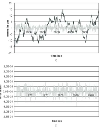
Figures 2a and b illustrate some results: While the errors of baselines lie within 5 cm, the errors of absolute ephemeris mount up to 15 cm. Thus, the application of baselines in
130 T. Reubelt et al.: Space Gravity Spectroscopy -20 -15 -10 -5 0 5 10 15 20 0 1000 2000 3000 4000 5000 time in s erro rs in cm -2,5E-04 -2,0E-04 -1,5E-04 -1,0E-04 -5,0E-05 0,0E+00 5,0E-05 1,0E-04 1,5E-04 2,0E-04 2,5E-04 970 1970 2970 3970 4970 time in s erro r in m /s ² a) b)
Fig. 2. (a) simulated errors of the tracked coordinates (dark) and baselines (grey) in cm and (b) errors of Newton interpolated accel-erations in m/s2(9-point scheme; 1t = 30 s); standard deviation
σx = 10 cm and correlation ρ = 0.993 = 0.970299 of absolute
ephemeris; one revolution of the CHAMP-satellite.
Newton interpolation will improve the accuracy. The errors of the Newton interpolated accelerations obtained from a 30 s sampling time lie within an accuracy of a few mGal. Due to the immense amount of observations from a 5 years mission duration of CHAMP this accuracy is sufficient to estimate a long wavelength geoid with an accuracy of at least one dm, as estimated from simulations (Reubelt et al., 2002). More details on the derivation of the vector-valued second order functional of Newton’s interpolation formula can be found in Austen and Reubelt (2000) and Austen et al. (2002).
5 System of equations
After the determination of the satellite’s acceleration vec-tor by means of Newton’s interpolation formula we have to compute the gradient of the gravitational Potential in the IRF. Therefore the partial derivatives of the gravitational po-tential U (λ, φ, r), Eq. (1), w.r.t. the spherical coordinates
(λ, φ, r) have to be determined, which are transformed in partial derivatives w.r.t. Cartesian BRF coordinates by means of the chain rule. Subsequently this Cartesian gradient is ro-tated into the IRF by means of the rotation matrix RT, where it is balanced by Newton’s law of motion with the satellite’s
0,00E+00 5,00E-10 1,00E-09 1,50E-09 2,00E-09 2,50E-09 3,00E-09 3,50E-09 4,00E-09 0 5 10 15 20 25 30 35 40 45 50 degree de gr ee vari an ces
standard deviation RSO-EGM96 RSO-GRIM5_S1 RSO-GRIM5_C1
Fig. 3. Degree variances of the estimated standard deviation and the differences between the recovered coefficients and various existing gravity models.
acceleration vector. The resulting linear system of equations is solved for the spherical harmonic coefficients by apply-ing a least squares adjustment in terms of a Gauss-Markov model.
6 Results
In this section we provide some results that have been ob-tained from an analysis of preliminary real CHAMP orbit data sets. The model error as well as accuracy estimates from error simulations of our method have already been tested in previous papers by Austen and Reubelt (2000), Austen et al. (2002) and Reubelt et al. (2002). There, a RMS of the geoid for an error-free simulation of a 1-week-arc (model-error) in the sub-mm range for degree/order 30/30 was ob-tained, which is sufficient for CHAMP-data analysis. From an error simulation study with the variance of coordinates
σX = 10 cm and the correlation of ρ = 0.99, which seems
to be a realistic for kinematic orbits according to Reubelt et al. (2002) a RMS of the geoid of 23 cm was received. Re-garding the complete CHAMP-mission, a geoid accuracy of below 10 cm seems to be possible, which is at least a con-firmation of present geoid models. An improving quality of kinematic orbits gives rise to hope for a higher geoid accu-racy (Svehla and Rothacher, 2002b). In order to obtain a first insight in real data processing with the proposed method, we have analysed two short preliminary CHAMP orbit data sets in this section.
First we have analysed the CHAMP RSO (Michalak et al., 2002) in the period of 1 July – 16 August 2001, which is sampled in the interval of 1t = 30 s. The CHAMP RSO is a dynamic orbit based on a taylored GRIM5-C1 (Gruber et al., 2000) model, thus the determined accelerations of the RSO will be highly correlated to GRIM5-C1. The estimated gravity field model should be comparable to GRIM5 C1, and therefore we have made comparisons to this model. Due to a good condition number of the normal matrix of about 700, no regularisation had been applied. For a first case study the Newton interpolated accelerations were not reduced from
T. Reubelt et al.: Space Gravity Spectroscopy 131
[m²/s²]
Fig. 4. Difference between recovered geopotential from a 45-days CHAMP-RSO and GRIM5 C1 up to degree/order 50/50 on the surface of a reference Earth with R = 6371 km; without c20term; RMSP ot=2.8 m2/s2
disturbing gravitational accelerations (third body attraction of sun, moon, other planets, ocean tides, solid Earth tides
. . .). Their effect on the geopotential is considered to be in the size of 1–2 m2/s2 ∼= ˆσgeoid = 10 cm (in general) with
maximum values of 10 m2/s2 ∼= ˆσgeoid = 1 m.
Further-more, the accelerometer measurements are omitted, since they still contain large biases. After publication of these bi-ases by GFZ (GeoForschungsZentrum Potsdam), the reduc-tion of non conservative disturbing accelerareduc-tions measured by the accelerometer will be carried out. Another possibility, which is in discussion, is the estimation of the accelerome-ter biases together with the spherical harmonic coefficients in one adjustment. The effect of negligence of the accelerom-eter measurements is about the same as the influence of the disturbing gravitational forces.
Figure 4 illustrates the differences between the recov-ered geopotential from a 45-days CHAMP RSO and from GRIM5 C1 up to degree and order 50/50 on the surface of a reference sphere with R = 6371 km. The root mean square (RMS) of the difference is about 2.8 m2/s2, which corre-sponds to a RMS of geoidal undulations of 28 cm, while the
RMSof the difference of a recovery up to degree/order 30/30 is 1.4 m2/s2 (as expected due to a loss of signal strength, caused by the term (R/r)l) for higher degrees l at satellite altitude). This error is, as visible in the Fig. 4, mainly caused by the polar data gap due to the inclination of the CHAMP orbit. At the non-polar regions, the difference to GRIM5 C1 is smoother and mostly smaller than 1–2 m2/s2with the high-est errors in the mountain areas, for instance the Himalayas or the Andes, where the gravity field is rough. Small oscilla-tions may be caused by the aliasing effect, since the gravity field was solved only to a maximum degree L.
To exhibit the negative effect of signal loss and downward continuation, the differences to the GRIM5 C1 model up to degree/order 50/50 have also been computed at satellite alti-tude (h = 400 km). The recovered geopotential at satellite
altitude is smoother (RMSP ot = 1.1 m2/s2) than the
com-puted geopotential on the reference sphere. This is the ef-fect of the signal damping at satellite altitude by (R/r)l, thus the higher frequency parts can not be discovered by satel-lite measurements at least not by CHAMP, as accurate as by terrestrial measurements. Furthermore a well known fact is clarified: While the differences are small at satellite alti-tude, they grow very fast with decreasing altitude due to an enhancement of noise by downward continuation. The dif-ferences on the surface are 4.5 times higher than at satellite altitude.
Figure 3 presents the error degree-variances to various models (EGM96, GRIM5 C1 and GRIM5 S1; Biancale et al., 2000), as well as the estimated standard deviations of our computations. It shows that the recovered potential fits best to the GRIM5 C1 model. Especially the differences to the satellite-only model GRIM5 S1 are very high. That can be explained by lower accuracy and sensitivity of the former in-cluded satellite data as opposed to CHAMP data. The stan-dard deviation of the coefficients, which is estimated from the Gauss-Markov model is smaller than the differences to the previous models, which may be caused also by the er-rors of these previous models. Probably the erer-rors of the es-timated coefficients are higher than the standard deviation, which is very small due to the (smooth) dynamic determina-tion of the RSO.
Subsequently we have analysed kinematic orbits, which are more erroneous, but not based on a force model in terms of a gravity field, and thus will lead to an independent gravity field solution. For our investigations we took a real prelim-inary kinematic CHAMP orbit of a 11-days time period, 20 to 30 May 2001, sampled at 1t = 30 s, which was processed by means of zero difference carrier phase measurements by Svehla and Rothacher (2002a). In order to estimate the accu-racy of the kinematic orbit as well as the accuaccu-racy of the es-timated baselines and accelerations, we made a comparison
132 T. Reubelt et al.: Space Gravity Spectroscopy -1 -0,8 -0,6 -0,4 -0,2 0 0,2 0,4 0,6 0,8 1 39801, 18 45801, 18 51801, 18 57801, 18 63801, 18 69801, 18 75801, 18 81801, 18 time (TT) in [s] differ e nces in m
x_diff y_diff z_diff
-0,08 -0,06 -0,04 -0,02 0 0,02 0,04 0,06 0,08 39801,184 48801,184 57801,184 66801,184 75801,184 time in (TT) in [s] differences in [m] a) -2,00E-04 -1,50E-04 -1,00E-04 -5,00E-05 0,00E+00 5,00E-05 1,00E-04 1,50E-04 2,00E-04 time in [TT] difference in [m/s²] 17280.184 34560.184 51840.184 69120.184 b) c)
Fig. 5. (a) difference of absolute ephemeris, (b) difference of baselines (x-coordinate) and (c) difference of accelerations (x-coordinate) between CHAMP RSO and kinematic orbit (day 141/2001) in the qIRF.
to the (smooth) Rapid Science (dynamic) orbit. Figures 5a to c illustrate the differences of (a) absolute coordinates, (b) baselines and (c) accelerations between kinematic and Rapid Science orbit.
The accuracy of the RSO is estimated by an independent comparison to Satellite Laser Ranging (SLR) measurements as 11 cm (Michalak et al., 2002) while the accuracy of the kinematic orbit can be classified in the range of 10–15 cm by a comparison to SLR (Svehla and Rothacher, 2002a, b). A second possibility to obtain information about the quality of the RSO is overlap analysis. From the 2 h overlap intervals of the 14 h RSO arcs we estimate an accuracy of the absolute RSO coordinates of 30 cm (Fig. 6a), while the accuracy of
the RSO-baselines is 0.9 cm (Fig. 6b). Indeed, as the com-parison to SLR illustrates, the accuracy of the RSO is much better, since the dynamic orbits are less accurate at the over-lap intervals due to oscillation effects at the beginning and at the end of an arc. Thus, the accuracy of the baselines is even higher than the estimated 0.9 cm which means that they pro-vide ideal reference values for the evaluation of the kinematic orbit baselines. Figure 5a illustrates the differences between the kinematic orbit and the RSO, which are in the level of 22 cm. Though it is difficult to use this difference to estimate the real error level of the kinematic orbit due to errors in the RSO, we are able to extract from Fig. 5a that the errors of the kinematic orbit are far from being white noise (due to
T. Reubelt et al.: Space Gravity Spectroscopy 133 -1 -0,8 -0,6 -0,4 -0,2 0 0,2 0,4 0,6 0,8 1 79371, 18 83871, 18 38151, 18 42651, 18 83331, 18 3761 1,18 42111,18 82791, 18 time (TT) in [s] differ ences in [m ]
diff_x diff_y diff_z
-0,08 -0,06 -0,04 -0,02 0 0,02 0,04 0,06 0,08 79371, 18 83871, 18 38151, 18 42651, 18 83331, 18 3761 1,18 42111,18 82791, 18 time (TT) in [s] diffe re nc es in [m]
diff_dx diff_dy diff_dz
a) -6,0E-06 -4,0E-06 -2,0E-06 0,0E+00 2,0E-06 4,0E-06 6,0E-06 79371,18 83871,18 38151,18 42651,18 83331,18 3761 1,18 42111,18 82791,18 time (TT) in [s] differences in [m/s²] diff_ax b) c)
Fig. 6. (a) differences of absolute RSO ephemeris, (b) RSO-baseline ferences and (c) RSO acceleration dif-ferences as obtained from orbit overlaps of 6 arcs of CHAMP RSO (days 141– 143/2001) in the qIRF (5 overlap peri-ods with 2 hours), x-, y-, z-coordinates (bright grey, dark grey, black).
the smooth behaviour of the RSO). This becomes apparent in Fig. 5b where the differences of the baselines computed from the kinematic orbit and the RSO are plotted, which are in the level of 1.0 cm (if we disregard the few outliers) and which would have been in the dm – level for white noise.
Regarding the accuracy of the RSO baselines of at least 0.9 cm or better, the absolute accuracy of the kinematic orbit baselines lies within 1–2 cm. Taking a value for the base-line – accuracy of 1.5 cm and the absolute kinematic or-bit error (by the comparison to SLR) of 10 cm, we obtain from their ratio σ1Xi/σXi =
√
2√1 − ρ (resulting from er-ror propagation) a correlation coefficient of about ρ = 0.99, which we have applied in our simulations. From the RMS
of the difference of the accelerations between RSO and kine-matic orbit of 1.9997 m/s2 and the accuracy of RSO accel-erations of 1.7 · 10−6m/s2 estimated from overlaps we de-termine the accuracy of kinematic orbit accelerations in the level of 2 mGal, as obtained from simulations of Sect. 4.2. This should lead (Reubelt et al., 2002) to a geoid accuracy of at least 1 dm for the complete CHAMP mission, which is comparable to present day long-wavelength geoid models, and demonstrates in general the applicability of the proposed method. Further refinement of the method will eventually lead to a contribution in improving these geoid models.
For the sake of completeness, we present the statistics of the analyzed 11-days kinematic orbit:
134 T. Reubelt et al.: Space Gravity Spectroscopy
averaged differences of estimated coefficients between RSO and kinematic orbit of one degree
0,00E+00 5,00E-10 1,00E-09 1,50E-09 2,00E-09 2,50E-09 3,00E-09 3,50E-09 4,00E-09 0 3 6 9 12 15 18 21 24 27 30 33 36 39 42 45 48 degree di ffe re nc es
Fig. 7. Averaged differences of estimated spherical harmonic coefficients between kinematic and Rapid Science CHAMP orbit.
[m²/s²]
Fig. 8. Difference between recovered geopotential from a 11-days CHAMP-kinematic orbit and GRIM5 C1 up to degree/order 30/30 on the surface of a reference Earth with R = 6371 km; without c20term; RMSP ot =3.2 m2/s2.
– number of analyzed coordinate-triples: 27 360; number
of data-gaps: 635;
– number of determined acceleration-triples1: 25 853
– RMS of coordinates2/ baselines2/ accelerations2: 0.22285 m / 0.01047 m / 1.9997 · 10−5m/s2.
(1): baselines with a deviation of 0.1 m in comparison to RSO have been neglected
(2): RMS of differences between CHAMP RSO and CHAMP kinematic orbit
Figure 8 presents the difference between the recovered po-tential from the kinematic orbit and the GRIM5 C1 model up to degree/order 30/30. Obviously the estimated coefficients and the recovered potential from the kinematic orbit are nois-ier than those from the analysis of the Rapid Science orbit, but we have to notice that the kinematic orbit data set was shorter than the RSO data set. The highest differences seem to be in the regions of rough gravity field as for example the Andes or the Himalayas, but also in other areas bigger dif-ferences are visible. For the estimation up to degree/order
30/30 the recovered potential differs from GRIM5 C1 by
RMSP ot=3.2 m2/s2, which corresponds to a RMS of geoid
differences of ∼30 cm. If the kinematic orbit is analysed to a higher degree/order, for instance 50/50, the RMS increases to RMSP ot =9.5 m2/s2, which means a RMS of geoid
dif-ferences of almost 1 m. This is stated by Fig. 7, where we can extract the errors of the coefficients to degree 30 in the level of 1 · 10−10−1 · 10−9, while they are increasing for higher degrees. We have to keep in mind, that only a 11-days kine-matic CHAMP arc has been analysed. The investigation of longer and more accurate arcs will lead to a higher accuracy, even for the coefficients of higher degree.
7 Conclusions
First results from preliminary real CHAMP orbits by means a gravity field determination approach based on determined accelerations from a LEO satellite orbit are presented in this contribution to demonstrate arising problems with the method and the achievable accuracy. A numerical differen-tiation scheme is applied to determine the accelerations. To
T. Reubelt et al.: Space Gravity Spectroscopy 135
minimize noise amplification due to differentiation, baselines instead of absolute ephemeris are introduced, which can be determined more accurate since kinematic orbits are highly correlated. The RMS of the accelerations lies within 1– 2 mGal, which leads to a long-wavelength geoid accuracy in the range of 20 cm from 1-week-arcs, as estimated from sim-ulations in previous papers. Thus from the whole CHAMP-mission, a long- wavelength geoid accuracy of at least 1 dm can be expected. The analysis of a preliminary 10-days kine-matic CHAMP orbit leads to a lower accuracy of 30 cm. Since an improvement of kinematic orbits is expected in the near future (Svehla and Rothacher, 2002b), from the whole CHAMP mission also a geoid accuracy of at least 1dm is expected, which is at least a confirmation of state of the art models. But an improvement of existing gravity field models seems at the moment hard to realize. A comparison between the proposed method and existing approaches has to be done to demonstrate if our algorithm can compete, in particular if and which parts of the gravitational field can be determined better. Future research should focus mainly on noise reduc-tion in the process of accelerareduc-tion determinareduc-tion, for instance by means of smoothing interpolation functions or regression methods, since the accuracy level of 1–2 mGal still seems to high.
References
Austen, G. and Reubelt, T.: R¨aumliche Schwerefeldanalyse aus semi-kontinuierlichen Ephemeriden niedrigfliegender GPS-vermessener Satelliten vom Typ CHAMP, GRACE und GOCE, M. Sc. Thesis, Geodetic Institute, University of Stuttgart, Ger-many, 2000.
Austen, G., Grafarend, E. W., and Reubelt, T.: Analysis of the Earth’s Gravitational Field from Semi-Continuous Ephemeris of a Low Earth Orbiting GPS-Tracked Satellite of Type CHAMP, GRACE or GOCE, in: International Association of Geodesy Symposia, Vol. 125, Vistas for Geodesy in the New Millennium, (Eds) Adam, J. and Schwarz, K. P., Axel Springer Verlag, 2002. Belikov, M. V. and Taybatorov, K. A.: An efficient algorithm for
computing the Earth’s gravitational potential and its derivatives at satellite altitudes, Manuscr. Geod. 17, 104–116, 1992. Biancale, R., Balmino, G., Lemoine, J. M., Marty, J. C., Moyno,
B., Barlier, F., Exertier, P., Laurain, O., Gegout, P., Schwintzer, P., Reigber, Ch., Bode, A., Gruber, Th., K¨onig, R., Massmann, F. H., Raimondo, J. C., Schmidt, R., and Zhu, S. Y.: A new
global Earth’s gravity field model from satellite orbit perturba-tions: GRIM5-S1, Geophys. Res. Lett., 27, 3611–3614, 2000. Engeln-M¨ullges, G. and Reutter, F.: Numerische Mathematik f¨ur
Ingenieure (Numerical mathematics for engineers), BI Wis-senschaftsverlag, Mannheim-Wien-Z¨urich, 1988.
Grafarend, E. and Vancek, P.: On the weight estimation in level-ing, National Oceanic and Atmospheric Adminstration (NOAA), Report NOS 86, NGS 17, Rockville, 1980.
Gruber, T., Bode, A., Reigber, Ch., Schwintzer, P., Balmino, G., Bancale, R., and Lemoine, J. M.: GRIM5-C1: combination solu-tion of the global gravity field to degree and order 120, Geophys. Res. Lett., 27, 4005–4008, 2000.
Hartmann, T. and Wenzel, H. G.: The HW95 tidal potential cata-logue, Geophys. Res. Lett., 22, 24, 3553–3553, 1995.
King-Hele, D.: Satellite orbits in an atmosphere: theory and appli-cations, Blackie Ltd, Glasgow, London, UK, 1987.
Koop, R. and Stelpstra, D.: On the computation of the gravitational potential and its first and second order derivatives, Manuscr. Geod. 14, 373–383, 1989.
Lemoine, F. G., Kenyon, S. C., Factor, J. K., Trimmer, R. G., Pavlis, N. K., Chinn, D. S., Cox, C. M., Klosko, S. M., Luthcke, S. B., Torrence, M. H., Wang, Y. M., Williamson, R. G., Pavlis, E. C., Rapp, R. H., and Olson, T. R.: The NASA GSFC and NIMA Joint Geopotential Model, NASA Goddard Space Flight Center, NASA/TP-1998-206861, Greenbelt, Maryland, USA, 1998. McCarthy, D. D.: IERS Conventions 1996, IERS Technical Note
21, Observatoire de Paris, Paris, France, 1996.
Michalak, G., Baustert, G., Koenig, R., and Reigber, Ch.: CHAMP Rapid Science Orbit Determination – Status and Fu-ture Prospects, in: First CHAMP Mission Results for Gravity, Magnetic and Atmospheric Studies, (Eds) Reigber, c., L¨uhr, H., and Schwintzer, P., 98–103, Axel Springer-Verlag, 2003. Reubelt, T., Austen, G., and Grafarend, E. W.: Harmonic analysis
of the Earth’s gravitational field by means of semi-continuous ephemeris of a Low Earth Orbiting GPS tracked satellite – case study: CHAMP, J. Geodesy, in press, 2003.
Svehla, D. and Rothacher, M.: Kinematic Orbit Determination of LEOs Based on Zero or Double-difference Algorithms Using Simulated and Real SST GPS Data, in: International Association of Geodesy Symposia, Vol. 125, Vistas for Geodesy in the New Millennium, (Eds) Adam, J. and Schwarz, K. P., Axel Springer Verlag, 2002a.
Svehla, D. and Rothacher, M.: Kinematic and reduced-dynamic precise orbit determination of low earth orbiters, Adv. Geo-sciences, 1, 47–56, 2003.
Wahr, J.: Earth tides, Global Earth physics, AGU Reference Shelf 1: 40–45, 1995.
![Fig. 1. Interpolation errors of Newton interpolated accelerations X for one simulated CHAMP revolution based on EGM96 up to degree/order 50/50; sampling time 1t = 30 s; 9-point scheme; x-axis: time in [s]; y-axis: acceleration error in [m/s 2 ]](https://thumb-eu.123doks.com/thumbv2/123doknet/14761239.585264/3.892.92.802.94.351/interpolation-newton-interpolated-accelerations-simulated-revolution-sampling-acceleration.webp)