Tidal signatures in mesospheric turbulence

(1)

HAL Id: hal-00317951

https://hal.archives-ouvertes.fr/hal-00317951

Submitted on 23 Mar 2006

HAL is a multi-disciplinary open access

archive for the deposit and dissemination of

sci-entific research documents, whether they are

pub-lished or not. The documents may come from

teaching and research institutions in France or

abroad, or from public or private research centers.

L’archive ouverte pluridisciplinaire HAL, est

destinée au dépôt et à la diffusion de documents

scientifiques de niveau recherche, publiés ou non,

émanant des établissements d’enseignement et de

recherche français ou étrangers, des laboratoires

publics ou privés.

Tidal signatures in mesospheric turbulence

C. M. Hall, S. Nozawa, A. H. Manson, C. E. Meek

To cite this version:

C. M. Hall, S. Nozawa, A. H. Manson, C. E. Meek. Tidal signatures in mesospheric turbulence.

Annales Geophysicae, European Geosciences Union, 2006, 24 (2), pp.453-465. �hal-00317951�

(2)

Ann. Geophys., 24, 453–465, 2006 www.ann-geophys.net/24/453/2006/ © European Geosciences Union 2006

Annales

Geophysicae

Tidal signatures in mesospheric turbulence

C. M. Hall1, S. Nozawa2, A. H. Manson3, and C. E. Meek3

1_{Tromsø Geophysical Observatory, University of Tromsø, 9037 Tromsø, Norway} 2_{STELab Nagoya University, Chikusa-ku Nagoya 464-01, Japan}

3_{Institute of Space and Atmospheric Studies, University of Saskatchewan, Saskatoon, SK S7N 5E2, Canada}

Received: 29 April 2005 – Revised: 22 December 2005 – Accepted: 3 January 2006 – Published: 23 March 2006

Abstract. We search for the presence of tidal signatures

in high latitude mesospheric turbulence as parameterized by turbulent energy dissipation rate estimated using a medium frequency radar, quantifying our findings with the aid of cor-relation analyses. A diurnal periodicity is not particularly evident during the winter and spring months but is a striking feature of the summer mesopause. While semidiurnal varia-tion is present to some degree all year round, it is particularly pronounced in winter. We find that the maximum in the sum-mer 24-h variation corresponds to that of the westward phase of the diurnal tide, and that the maximum in the winter 12h variation corresponds to that of the southward phase of the semidiurnal tide. This information is used to infer the hor-izontal propagation direction of gravity waves: during the summer the eastward direction is consistent with closure of the summer vortex, while in winter the inferred directions require more complex arguments.

Keywords. Meteorology and atmospheric dynamics

(Mid-dle atmosphere dynamics; Turbulence; Waves and tides)

1 Introduction

While relatively little work has been done earlier on tidal sig-nature in turbulent intensity, coupling between Gravity Wave (GW) flux and/or momentum transport and waves of periods including 12 h, 24 h, 2 d and 16 d (Manson et al., 1998; Fritts and Vincent, 1987; Thayaparan et al., 1995, Holdsworth et al., 2001; Manson et al., 2003) has received considerable at-tention. These authors (and via references within) variously explain how, when the background wind speed |u| defined as the summation of the mean wind and all wave perturba-tions other than the GW in question (normally assumed to be planetary waves and tides), opposes the GW sufficiently, the GW will saturate. Saturation is quantified by violation of the condition that the perturbation velocity of the GW, u0_>c−u_,

c being the GW’s phase velocity (c−u being the intrinsic

Correspondence to: C. M. Hall

(chris.hall@tgo.uit.no)

phase velocity) (e.g. Fritts, 1984), and that then u0 is pro-portional to c−u. Thus saturation is most likely when u op-poses c and furthermore when the mean wind is augmented by contributions from other dynamics such as in-phase per-turbations from tides and planetary waves. Following, for example, Manson et al. (1998), in winter, westward propa-gating GWs predominate around the mesopause, the mean eastward winds lower down having filtered out the eastward propagating population. Increases in the GW-related wind variances then occur and maximize when the tide perturba-tions are eastward. The reverse is true for the summer, when the eastward propagating GWs survive the westward meso-spheric jet, and when they saturate, they drag the westward wind back across to eastward, thus closing the jet near 90 km (also see, for example, McLandress, 1998). The GW wind variances then maximize when the tidal wind is westward.

From the above scenario, therefore, we can expect 12-h and 24-h modulations of turbulent energy dissipation rates and it is these that we shall search for here. Two basic methodologies dominate investigation of turbulence in the mesosphere: in situ using rocket borne probes (e.g. L¨ubken, 1996) and radar (e.g. Hocking, 1996). These two approaches have often yielded somewhat different results, presumably due to the radically different sampling scales (Danilov and Kalgin, 1996). One way of escaping from this dilemma has been to accept that the radar method may deliver “up-per limit” estimates of turbulent intensity and rather to focus on the variability of turbulence, for example, as a function of season, rather than the absolute values themselves (Hall et al., 1999). In practice, it is common to combine several in situ soundings with radar and other ground-based measure-ments to measure as many atmospheric parameters as pos-sible over a short time interval in order to minimize ambi-guities due to non-stationarity; on the other hand, radar ob-servations may be used as day averages recorded over sev-eral years in order to investigate climatologies. Nevertheless, L¨ubken (1997) investigated seasonal variation using data from numerous in situ soundings. In this study, however, we shall investigate phenomena between these timescales: vari-ability of turbulence over timescales of 1 day or less, and how

(3)

454 C. M. Hall et al.: Tidal signatures in mesospheric turbulence

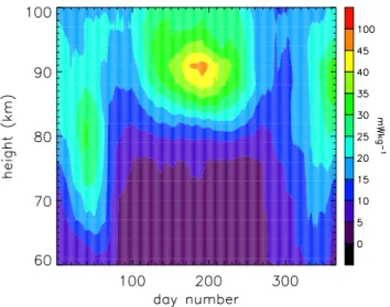
Fig. 1. Energy dissipation rates in mWkg−1 for 2004 from the Tromsø MFR. A 30-day wide boxcar has been run through the data at each height for illustrative purposes.

this variability itself varies with season. Tidal response of turbulence has been addressed earlier by Hall (1998), (while investigating whether ε0 might be determined from incoher-ent scatter data), Hall et al. (2003a), Holdsworth et al. (2001) and recently by Roper and Brosnahan (2005), but otherwise has been little touched upon.

The instrument used to provide data for this study is the Tromsø medium frequency radar (Tromsø MFR) located at 70◦N 19◦E in Northern Norway. The radar has earlier been described by Hall (2001); it operates at 2.78 MHz and the al-titude and time resolutions for the purpose of this study are 3 km and 5 min, respectively. An absolute altitude calibra-tion has been performed very recently by Hall and Husøy (2004). The so-called “full correlation analysis” method of data reduction has been described in full by Meek (1980) and Briggs (1984), and the means of estimating turbulent energy dissipation rate, ε, has been described by Hall et al. (1988). Although we shall present data up to 100 km here, it should be noted that group delay of the 2.78-MHz radio wave may occur, normally restricted to altitudes over 90 km, rendering these heights “virtual” (e.g. Namboothiri et al., 1993).

As we have touched upon above, there is some question as to whether the estimate of turbulent energy dissipation rate is truly representative of ε, and hereafter, therefore, we shall denote the values obtained by the radar method by ε0_{. For}

a deeper treatise of the assumptions and pitfalls inherent in estimation of ε the reader is referred to the complementary papers of Hocking (1999) and Hall et al. (1999). Since lit-tle is known of inter-annual variation of turbulent intensity in, at least, the upper mesosphere, at the level of seasonal variations of monthly means at these latitudes, we have cho-sen to use data from one year initially (2004). We shall be

Fig. 2. Energy dissipation rate averages for each hour and month,

with monthly (0:00–24:00 UT) means subtracted, for selected heights. Pinks are maxima, greens are minima.

comparing turbulence variability with corresponding neutral wind tidal amplitudes and phases, and the latter are known to exhibit modest inter-annual changes, again at the level of sea-sonal variations of monthly means at these latitudes. As an example, the strong seasonal variations of 12- and 24-h tidal amplitudes/phases evident in the height versus time contour plots in Manson et al. (2004) are reproduced on an annual ba-sis with only modest changes (from a visual inspection of the aforementioned color plots). The largest variations that do occur are typically associated with stratospheric warmings, but even these lead to only minor distortions of the contours in such plots. These features are interesting and significant, of course, but not an issue for studies of the type we engage in here. A further reason for only selecting the 2004 data is that the co-located Nippon/Norway Tromsø Meteor Radar (NTMR) has been operating since the end of 2003, such that the complete year 2004 data from this instrument are avail-able for comparison (indeed the Tromsø MFR and NTMR 2004 data were compared when re-calibrating the altitudes for the MFR operation).

(4)

C. M. Hall et al.: Tidal signatures in mesospheric turbulence 455

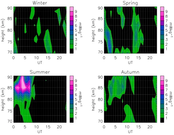
Fig. 3. Energy dissipation rate averages for each hour and season and with the seasonal means subtracted, as a function of UT and height,

and for each of the seasons, defined as winter = November, December and January, etc.

2 Data reduction and post-analysis

The 2004 ε0_{dataset is shown in Fig. 1 for reference. Features}

include a summer maximum above the mesopause with little turbulence below and almost altitude independent turbulence during the maximum of the winter half year; this seasonal variation is typical behaviour, as demonstrated by L¨ubken (1997) and Hall et al. (1999). While the data overview shown in Fig. 1 involves considerable temporal smoothing, the orig-inal time resolution is 5 min as stated earlier. In order to in-vestigate timescales corresponding to tidal modes, we have sorted the data into 1-month×1-h bins and averaged (i.e. 00:00–01:00 UT for January etc., 288 averages altogether) for each height in the range (60–100) km. Since we are look-ing for tidal signatures specifically, we have then subtracted the day-averages for each month and height from the corre-sponding 00:00–24:00 UT series. These residuals, for 3 se-lected heights, 79, 85 and 91 km, are shown in Fig. 2. At 85 km (centre panel) during summer we note a clear diurnal variation with a maximum in the early morning of around 15 mWkg−1, but little obvious variation in autumn and win-ter (upper part of the 85-km panel). At 91 km (top panel) there is a similar but less well-defined picture. At 79 km (bottom panel) variation is considerably weaker, but with the near-absence of the summer diurnal variation to dominate the

plot, the late winter (February) semidiurnal mode comes to the fore.

Categorizing November, December, January as winter, February, March, April as spring, May, June, July as sum-mer and August, September, October as autumn, we can look at the altitude variation as a function of UT for each of the four seasons (Fig. 3). The dominating feature is the summer diurnal variation at the (summer) mesopause. The autumn picture is somewhat similar but lacking the large amplitude at 85 km. In spring and winter, the picture is somewhat con-fused, although, in spring at least, below 80 km the double peaks suggest semidiurnal variation.

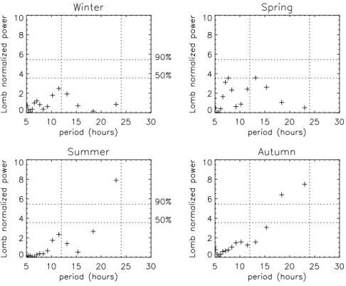
Since the seasonal synopses indicate pronounced features around 85 km, let us investigate the spectral characteristics more quantitatively. Performing Lomb-Scargle analyses us-ing the implementation by Hocke (1998) we arrive at the discrete spectra for frequencies associated with tidal motion and with associated confidence levels, shown in Fig. 4. The winter, spring – summer, autumn difference is striking. In winter and spring there is little evidence of a diurnal vari-ation, whereas in summer and autumn the 24-h periodicity dominates. Indeed, from the Lomb-Scargle analysis we see that only the summer and autumn 24-h period powers ex-ceed the 50% significance limit. If we extend the spectral

(5)

Fig. 4. Lomb-Scargle periodograms for 85 km for each of the seasons defined earlier. 12- and 24-h periods are indicated by dotted ordinates.

Significance levels of 50 and 90% are also indicated by dotted abscissae.

(6)

Fig. 6. Comparisons between tides in the neutral zonal wind and ε0for 85 km and for the four seasons. The solid line depicts ε0, the dotted line shows the 24-h component, the dashed line the 12-h component, and the dot-dashed line the combination of these. Note that times are in UT, 00:00 UT being 01:17 LST. Positive wind values are eastward.

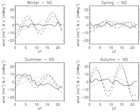
Fig. 7. As for Fig. 6 but for the meridional wind. Positive wind values are northward.

analysis to other altitudes, we obtain the synopses shown in Fig. 5. Note that, comparing with Fig. 4, the contour inter-vals 5–6 and 3–4 correspond to 90% and 50% confidence levels respectively and can be identified by the keys. In

win-ter, a ∼12-h variability is evident around 83 km, although with a low confidence level. In spring, a ∼12-h variability maximises near 77 km exceeding 90% confidence between 74 and 82 km. In summer, the 24-h periodicity dominates

(7)

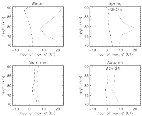
Fig. 8. Altitude profiles of hours of maximum of 12- and 24-h periods in ε0for each of the four seasons. The time-axis, in UT, extends from –12 to +24 to avoid “wrapping” of the phase. The dotted line denotes 24 h and the dashed line 12 h.

Fig. 9. Altitude profiles of hours of maximum of 12- and 24-h periods in westward wind component for each of the four seasons. Again, the

time-axis, in UT, extends from –12 to +24 to avoid “wrapping” of the phase. The dotted line denotes 24 h and the dashed line 1 h.

with over 90% confidence at all heights shown, although a

∼10-h contribution is with 50% confidence is evident at the summer mesopause. In autumn dominant periodicities are

less evident: there is a similarity with the summer (>90% confidence) picture above 80 km and with the winter picture (>50% confidence) below 80 km, which together could be

(8)

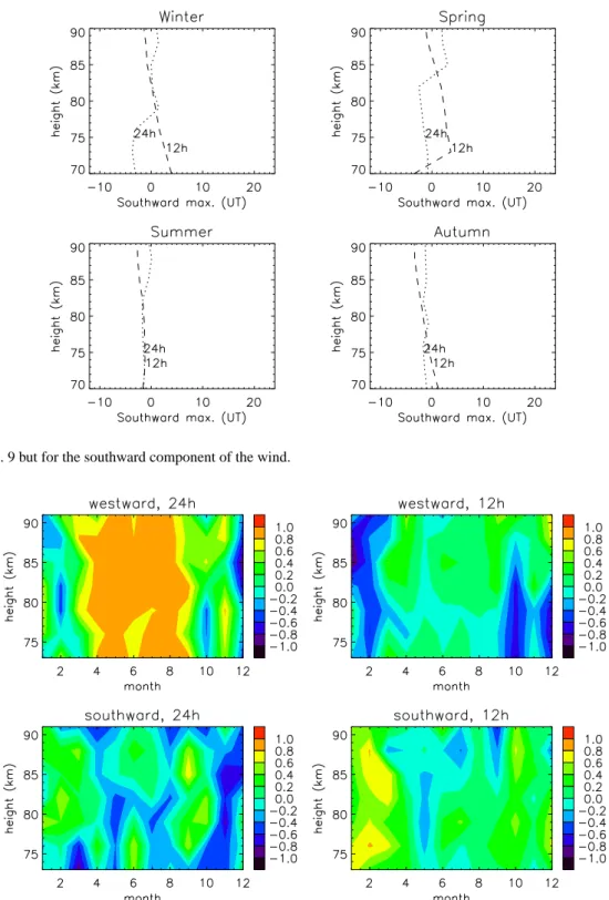
Fig. 10. As for Fig. 9 but for the southward component of the wind.

Fig. 11. Spearman’s rank correlation coefficients for monthly averages of daily variation of ε0with each of the westward 24-h, westward 12-h, southward 24-h, and southward 12-h tidal wind components.

interpreted as a transition from summer to winter states. Fi-nally, it is interesting to note the 50% confidence level ter-diurnal (7–8 h) feature in winter (below ∼75 km) and spring above ∼75 km.

Hitherto, we have established the presence of 12-h and 24-h periods in the data. In order to relate these to tidal features in the wind field we must substantiate our findings with phase information, so again, looking first at 85 km, we

(9)

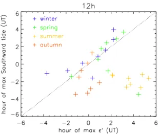
Fig. 12. Hour-of-maximum scatter plots of 12-h southward tide

versus 12-h ε0. A dotted line indicates unity slope. Symbols are coded according to season, as indicated on the figure.

Fig. 13. As for Fig. 12 but for 24-h westward tide.

have ε0 examined the variation of over 24 h for each season in relation to the zonal (Fig. 6) and meridional (Fig. 7) tidal 12-h, 24-h and 12-h+24-h components from the same radar. Note that we have retained UT as our reference time – local solar time leading UT by 1 h 17min. Any clear relation be-tween 12-h features is difficult to discern, however, for sum-mer and to a lesser degree, autumn, we note a correlation be-tween the westward phase of the wind (i.e. zonal component negative) and turbulent intensity, in agreement with the cor-relation reported by Holdsworth et al. (2001). To quantify this we have determined Spearman’s rank correlation coef-ficients and significances. Referring to Fig. 6, for summer the correlation coefficient between the westward 24-h tidal wind and turbulent intensity was found to be 0.77 with better than 95% confidence while for autumn the correlation coef-ficient was 0.74, again with better than 95% confidence. As

a comparison (i.e. Fig. 7) the corresponding correlation coef-ficients for the meridional component were found to be only 0.04 (15% confidence) and 0.14 (46% confidence), respec-tively.

Extending this approach to more heights, we have ob-tained altitude-profiles of hour of maximum of each of 12-h and 24-h periods only of variation of ε0, again using Hocke’s implementation of the Lomb-Scargle periodogram analysis, and as before, for each season (Fig. 8). Similarly, we have obtained corresponding profiles of the hours of maximum of diurnal and semidiurnal tides for all four seasons, and for north, south, east and west phases, since, as we have seen, in summer, there is a correspondence between times of max-ima in the westward phase of the diurnal tide and diurnal variation of ε0. The phases (i.e. hours of maxima) of the southward and westward components of the 12-h and 24-h tides are shown in Figs. 9 (westward) and 10 (southward), again for all four seasons. We see a notable correspondence between 24-h period westward component (and also for the sum of 12- and 24-h tides) and the corresponding profile for

ε0 in summer and a similarity for 12 h southward in winter and spring, whereas corresponding northward and eastward phases failed to reveal any similarities (thus we have not in-cluded them here). We now need to quantify these findings and have therefore extracted monthly means of daily varia-tions of ε0 and westward and southward tidal wind compo-nents. Again, using Spearman’s rank correlation method, we have obtained monthly height profiles of correlation coeffi-cient for correlations between sets of 24-hourly values of ε0 and each of 24-h westward, 12-h westward, 24-h southward, and 12-h southward tidal components (Fig. 11). The direc-tions of the tidal wind components (i.e. westward and south-ward) have simply been chosen such that the correlation co-efficients, anticipated from the preceding qualitative assess-ment, will be positive. Indeed we see strong (>0.8) corre-lation between turbulent intensity and the westward phase of the tide between March and September at all heights between 73 and 91 km (top left panel of Fig. 11). We also see clearly the high (>0.6) correlation between turbulent intensity and the southward phase of the tide between January and March at all heights between 73 and 90 km (bottom right panel of Fig. 11). Other correlations, more limited in height extent and duration are present, for example in January ε0 corre-lates with the eastward 12-h component around 86 km and with the westaward 24-h component at selected heights in November.

Focussing on the dominant two correlations we identified in Fig. 11, in order to provide an additional visualization, we have produced scatter plots for the southward maxima versus corresponding ε0phase for the 12-h period (Fig. 12) and for the westward maxima versus corresponding ε0phase for the 24-h period (Fig. 13), coding the symbols according to sea-son. Recalling the indication of a semidiurnal signature in ε0 for winter and spring only we see that clustering around the unity slope for Fig. 12 largely originates from these seasons

(10)

and, to a lesser extent, autumn, (consistent with the bottom right panel of Fig. 11). On the other hand, summer was char-acterized by a diurnal signature in ε0_{, and indeed, in Fig. 13,}

only summer data cluster around the unity slope, the other seasons, including autumn, exhibit considerable scatter (con-sistent with the top left panel of Fig. 11). Other correspon-dences of tidal perturbation maxima and epsilon were not initially visually persuasive, but other evidence is considered below in the discussion, which expands the correlation ex-amples.

3 Discussion

We can put the observations described above into context of the gravity wave/tidal interaction described in the Introduc-tion as follows.

First we examine the summer case:

1. Gravity wave propagation is predominantly eastward, closing the mesospheric jet, the drag starts from typi-cally 70 km and closure is 90 km or above;

2. Prevailing wind is westward below 85–90 km;

3. Gravity wave saturation is most pronounced during the westward phase of the tide as c−u is now very large (since u is large and negative) and so is u0 (since the wave amplitudes are allowed to grow exponentially); 4. From the observation, this is also the condition for

maximum turbulent energy dissipation and the 12+24-h tides add to give a large variable flow.

Here, the first three points above are known from previ-ous climatological studies, and the final point is suggested by the observations reported in this study. The conclusion from combining the summer observation with the GW satu-ration paradigm is that the diurnally occurring enhancements in energy dissipation rate arise from tidally induced grav-ity wave saturation (as opposed to any other gravgrav-ity wave dissipation/breakdown mechanism). The summer scenario and, gratifyingly, our interpretation agree with the findings of Holdsworth et al. (2001) wherein maxima in turbulent ve-locity correlate with maxima in zonal wind.

We should briefly comment on the other three seasons and their zonal components (Fig. 6) before addressing the winter case in more detail. In autumn, as discussed in Manson et al. (1998), an isotropic tropospheric GW source plus a lack of filtering of the GW at lower heights (weak vortex) will not lead to a modulation of the GW dissipation at a 12-h period due to a strong mesospheric 12-h tide: this is con-sistent with Fig. 6. However, it also still puzzled Manson et al. (1998) as to why there was not a strong autumnal mod-ulation of the GW, and they concluded that the GW sources were weaker, and more variable in direction and occurrence during the autumn. Similar arguments can be made for the

situation during Tromsø autumn and spring; but for the lat-ter, as the tide is weak, there is less urgency for an explana-tion! Finally, Fig. 6 indicates strong winter zonal 12-h tides along with weak variations in the turbulent intensity. We again look for some similarities with the above arguments for autumn and spring. However, the stratospheric vortex is strong and GW directional anisotropy is expected at meso-spheric heights – our expectation would have been for a 12-h modulation of the GW and the turbulent intensities. Inter-estingly, Manson et al. (1998) found a similar lack of winter response in the GW wind-variance, and concluded: “The in-termittent nature of the GW modulation (noted especially in winter) also strongly suggests that the wave sources are in-termittent in strength and direction and that the background wind at lower heights also contributes variability.”

Turning now to the winter case, involving the meridional component, we hypothesize:

1. From our summer case conclusion, maxima in turbu-lent energy dissipation arise from saturation due to tides augmenting prevailing wind;

2. From the observation, this saturation is at the southward phase of the 12-h tide;

3. Meridional mean wind is very slight. Because the underlying background winds are also weak, the directional anisotropy of the GW reaching the meso-sphere will be much less than for the EW winds. Hence our expectation is for weaker GW modulation and also that of the turbulent intensity. The NS modulations in Manson et al. (1998) were also somewhat less clear than for the EW.

Our observations are complemented by those of Espy et al. (2004a) who reported GW momentum flux variation mod-ulated by, and out of phase with, the meridional tide in the Antarctic winter. From this train of thought, the conclusion for the winter case is that the gravity wave propagation di-rection must have a northward bias, so that c−u is again maximized. However, we note that while the phase relations are clear in Figs. 8 and 10, the amplitudes of these modu-lations are weak (Fig. 7). Although Hall et al. (2003b) ob-served ageostrophic flow in winter (1996–2002): cyclonic flow around the pole combined with divergence. 2004 was pathological in relation to the 1997–2002 mean, as we shall see. To create the 1997–2002 mean flow picture, the east-ward flow must be accelerated and/or given an equatoreast-ward momentum deposition due to GWs such that the flow over-comes the poleward pressure gradient force, viz. eastward and/or southward GW propagation, and this is incompatible with our provisional winter case conclusion above.

From Manson et al. (2003) (and translating Espy et al. (2004b) Antarctic climatology to the Northern Hemi-sphere) we expect dominantly westward propagating GWs

(11)

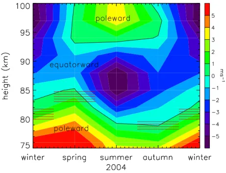
Fig. 14. Seasonal averages of meridional wind component for 2004 as a function of height as determined by the Tromsø MFR. The seasons

are defined as follows: winter = November, December, January, spring = February, March, April, summer = May, June, July, and autumn = August, September, October. Since purpose is to indicate the wind direction, only the zero contour is included; colour changes occur every 1 ms−1. Blue colours indicate southward/equatorward flow while green/orange indicate northward/poleward flow. The regions with horizontal hatching indicate the heights at which the Lomb-Scargle amplitude of ∼12-h periodicity in ε0exceeds the summer value (cf. Fig. 5).

throughout winter and until the end of March when the vor-tex (40◦–70◦N) begins to reverse. This is in order to deposit westward momentum and to drag the mean circulation/flow from eastward to the westward, which is required to close the winter vortex in the lower thermosphere. Indeed this GW flux is likely to continue through into April and cause the tongue of lower thermospheric westward flow (Manson et al., 2004), which is the mesospheric precursor to the summer mesospheric westward jet. We surmise that these processes occur during our spring generalization (when tidal signatures in turbulence are less evident), otherwise we could expect an analogy to the summer case: the eastward phase of the tide(s) augmenting the eastward mean wind and causing saturation in westward propagating GW and associated tidally modu-lated turbulence, something we do not see. From, for exam-ple, Fritts (1984) and Fritts and Alexander (2003), shedding of energy by GWs as they saturate is most likely by convec-tive instability and thereafter turbulence.

Proceeding with our explanation of the winter case, we must take into account the meridional wind component for 2004 and not the climatological picture of Hall et al. (2003b). In 2004 the mid-mesosphere poleward convergence extended further into the uppermost mesosphere than usual. We have constructed seasonal means of the meridional wind (i.e. where winter = November, December, January, spring = February, March, April, summer = May, June, July and

autumn = August, September, October, shown in Fig. 14. Here, we are primarily interested in the direction (poleward or equatorward) and not in the amplitudes themselves, and for that reason only the zero line is indicated. Note that only 2004 data are presented in this figure and the months “wrap”: contours are obtained from December 2004 (as opposed to 2003), January 2004,... December 2004, January 2004 (as opposed to 2005). Next, we have noted the heights below which the significance of the semidiurnal signature in ε0 ex-ceeds 50% (i.e. the intersections of the 12h ordinates with the Lomb normalized power =3.5 contour in each panel of Fig. 5) and indicated these on Fig. 14 as season-wide and 2 km deep hatchings. The proximities of these heights to the demar-cation line between poleward and equatorward flow is self-evident. We conclude, from Figs. 5 and 14, then that 12-h perturbations in turbulence occur outside the summer months and where the flow has poleward convergence. The phases of Figs. 8 and 10 are modestly consistent with this for the 3 sea-sons, but Fig. 14 was needed to encourage that interpretation beyond winter. In particular, for winter, the preponderance of correlation between 12-h periodicity in ε0 _{and the}

south-ward phase of the 12-h tidal perturbation of the meridional flow occurs when the meridional flow itself is northward.

We have also calculated the correlations between the to-tal wind variance (inertial gravity waves (periods of several hours), tides and planetary waves up to periods of 10 days)

(12)

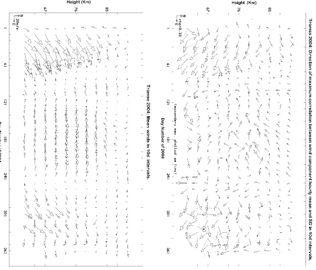
Fig. 15. Mean 10-d winds and correlation vectors (over 10 days) for the Tromsø MFR. The correlations are between the hourly mean winds

and their standard deviations over all azimuthal directions (see Sect. 3).

and the high frequency GW (10–150 min), using the method of C. E. Meek, which is described in Manson et al. (1999). Briefly, the hourly mean winds over 10-d intervals are cor-related with their standard deviations. These correlations are calculated for all directions 0–360◦ East of North. If there is a preferred direction (dominant correlation magni-tude) for GW propagation, and the waves are saturated, the simple model which has been used already in this paper, is used to infer the GW phase-speed directions. The 10-d mean wind vectors and the directions of maximum correlation are shown in Fig. 15 for the full year of 2004. Since wind pertur-bations in the direction of the correlation vectors have pro-duced the most significant control of GW variance, the GW phase propagation will be in the opposite direction to the cor-relation vectors. The argument is that same as that given at the beginning of this section. Considering the summer-centered months first, the westward correlation vectors in-fer a generally eastward GW propagation direction through-out the duration of the summer’s westward flow (late-April

to the end of August). This is consistent with the discus-sions above involving ε0 and tidal modulations, and the clo-sure of the summer westward vortex near 85 km. Finally for the winter-spring season, the 10-d mean winds during January and February are eastward and northward, as dis-cussed above in reference to Fig. 14. The inferred GW di-rections, from the correlation vectors, are westward, consis-tent with GW involved with closure of the winter vortex, and northward as again discussed above with reference to Fig. 14. The pattern during the autumn and early winter is less organized, although mainly eastward correlation vec-tors/westward GW propagation is inferred. Indeed, encour-aged by this, Fig. 9 shows an approximate out-of-phase cor-relation between westward phase (i.e. eastward) of the 12-h tidal perturbation and the epsilon periodicity, consistent with a westward flux of GW. We have, for winter:

1. Maximum turbulent energy dissipation when perturbed flow is southward (although the mean flow is northward and weak);

(13)

2. Gravity wave saturation is most pronounced during the southward phase of the tide, with indications of satura-tion also during the eastward phase;

3. Gravity wave propagation has a northward and west-ward component in addition to the westwest-ward character-istic shown by Manson et al. (2003).

The remaining puzzle is why the 12-h modulation of tur-bulence ceases at heights where there is equatorward mean flow. Examining dynamic instability alone (in the absence of measurements of Brunt-Vaisälä frequency), Hall et al. (2002) reported a tendency to large (i.e. >1) gradient Richardson Numbers (Ri) in the (Northern Hemisphere) summer and higher preponderance of Ri<0.25 (i.e. indicative of dynamic instability) at the equinoxes (winter data were not available that the time of the Hall et al. (2002) study). The deeper mesopause in summer results in greater lapse rates in the upper mesosphere in the summer months; it is well known that this low static stability causes expanded vertical wave-lengths of gravity waves and less instability, while strong mean stability favours strong gravity wave instability and tur-bulence. Therefore the summer arctic mesopause exhibits almost no turbulence while the very stable lower thermo-sphere exhibits very substantial turbulence, as demonstrated by Lübken (1997). Thus, furthering the approach of Hall et al. (2002) to give climatologies of Ri or possibly Froude Number, and perhaps exercising the viewpoint of Zink and Vincent (2004) to look into the relative probabilities of dy-namic and static stabilities as a function of height and sea-son, may help resolve the dilemma. The way forward is per-haps shown by Holdsworth et al. (2001) who investigated stability by deriving temperature gradients from GW ampli-tudes. However, through concurrent work, temperatures will be available directly from the co-located meteor wind radar and therefore we prefer to defer quantification of stability to a subsequent study. Finally, we should point out the dangers of generalization when predicting the characteristics of the GW flux arriving in the mesosphere from below and apply-ing them to any given observation site: geographic variation of dynamics over a (O)100-km baseline reported by Man-son et al. (2004) was attributed to differences in orographic forcing – particularly pertinent to the observations presented here.

4 Summary

We have searched for evidence of tidal (a priori 24 h and 12 h) signatures in high latitude mesospheric turbulence as a function of season, quantifying our findings with the help of correlation analyses. Our summer observations show that there is a diurnal variation in turbulent intensity maximizing when the wind perturbation due to the diurnal tide is west-ward (indeed the sum of the 24-and 12-h tidal perturbations

is perhaps better correlated). When the mean wind, west-ward in summer below 88 km, and the westwest-ward-wind phase of the diurnal tide combine, saturation of gravity waves, the predominant propagation being eastwards in summer, also maximizes. Saturating gravity waves shed energy into tur-bulence through convective instability, thus giving rise to the diurnal enhancements in turbulent energy dissipation rate we report here. In winter, our observations indicate that there is a weak semidiurnal variation in turbulent intensity maximiz-ing when the wind perturbation due to the semidiurnal tide is southward and eastward. The relative importance of the 12-h and 24-h tides during the different seasons may explain why it is the semidiurnal tide that modulates winter turbulence in contrast to the diurnal tide modulating summer turbulence. Moreover, a maximum in southward and eastward perturba-tions would coincide with a maximum in gravity wave satu-ration if the propagation directions were northward and west-ward. Azimuthally varying correlations between the total wind variance (periods up to 10 days) and the wind variance due to high frequency GW (10–150 min) are entirely consis-tent with this. Also, this meridional scenario is compatible with concurrent studies of gravity wave fluxes (M. Tsutsumi, private communication) and meridional flow for 2004. Fu-ture work will be required to address this aspect, conceiv-ably by investigating the climatology and seasonal behavior of turbulence production mechanisms.

Acknowledgements. The first author thanks the Norwegian Re-search Council for support. The Japanese author thanks the Min-istry of Education, Science, Sports and Culture, Japan, for a grant-in-aid for scientific research. The Canadian authors gratefully ac-knowledge grants from the University of Saskatchewan, and the In-stitute of Space and Atmospheric Studies and the national agency, NSERC.

Topical Editor U.-P. Hoppe thanks two referees for their help in evaluating this paper.

References

Briggs, B. H.: The analysis of spaced sensor records by correlation techniques, in: Handbook for MAP, 13. SCOSTEP, University of Illinois, Urbana, 166–186, 1984.

Danilov, A. D. and Kalgin, Y. A.: Eddy diffusion studies in the lower thermosphere, Adv. Space Res., 17, (11)7–(11)24, 1996. Espy, P. J., Jones, G. O. L., Swenson, G. R., Tang, J., and

Taylor, M. J.: Tidal modulation of the gravity-wave momen-tum flux in the Antarctic mesosphere, Geophys. Res. Lett., 31, doi:10.1029/2004GL019624, 2004a.

Espy, P. J., Jones, G. O. L., Swenson, G. R., Tang, J., and Taylor, M. J.: Seasonal variations of the gravity-wave momentum flux in the Antarctic mesosphere and lower thermosphere, J. Geophys. Res., 109, doi:10.1029/2003JD004446, 2004b.

Fritts, D. C.: Gravity wave saturation in the middle atmosphere: a review of theory and observations, Rev. Geophys. Space Phys., 22, 275–308, 1984.

(14)

Fritts, D. C. and Alexander, M. J.: Gravity wave dynamics and effects in the middle atmosphere, Rev. Geophys., 41(1), 1003, doi:10.1029/2001RG000106, 2003.

Fritts, D. C. and Vincent, R.A.: Mesospheric momentum flux stud-ies at Adelaide, Australia: observations and a gravity wave – tidal interaction model, J. Atmos. Sci., 44, 605–619, 1987.

Hall, C. M.: Tidal signatures in mesospheric kinetic energy dis-sipation rates determined by EISCAT, Geophys. Res. Lett., 25, 1941–1944, 1998.

Hall, C. M.: The Ramfjordmoen MF radar (69◦N, 19◦E): Appli-cation development 1990–2000, J. Atmos. Solar-Terr. Phys., 63, 171–179, 2001.

Hall, C. M., Meek, C. E., and Manson, A. H.: Turbulent energy dissipation rates from the University of Tromsø/University of Saskatchewan MF radar, J. Atmos. Solar Terr. Phys, 60, 437– 440, 1998.

Hall, C. M., Hoppe, U.-P., Blix, T. A., Thrane, E. V., Manson, A. H., and Meek, C. E.: Seasonal variation of turbulent energy dis-sipation rates in the polar mesosphere: a comparison of methods, Earth Plan. Space, 51, 515–524, 1999.

Hall, C. M., Aso, T., and Tsutsumi, M.: An examination of high latitude upper mesosphere dynamic stability using the Nippon /Norway Svalbard Meteor Radar, Geophys. Res. Lett., 29, 1211– 1213, 2002.

Hall, C. M., Nozawa, S., Meek, C. E., Manson, A. H., and Luo, Yi: Periodicities in energy dissipation rates in the auroral MLT, Ann. Geophys., 21, 787–796, 2003a,

SRef-ID: 1432-0576/ag/2003-21-787.

Hall, C. M., Aso, T., Manson, A. H., Meek, C. E., Nozawa, S., and Tsutsumi, M.: High latitude mesospheric mean winds: a comparison between Tromsø (69◦N) and Svalbard (78◦N), J. Geophys. Res., 108, 4598, doi:10.1029/2003JD003509, 2003b. Hall, C. M. and Husøy, B. O.: Altitude calibration of the Tromsø

Medium Frequency Radar, Tromsø Geophysical Observatory Report, University of Tromsø, Norway, 13, 2004.

Hocke, K.: Phase estimation with the Lomb-Scargle periodogram method, Ann. Geophys., 16, 356–358. 1998.

Hocking, W. K.: An assessment of the capabilities and limitations of radars in measurements of upper atmosphere turbulence, Adv. Space Res., 17, (11)37–(11)47, 1996.

Hocking, W. K.: The dynamical parameters of turbulence theory as they apply to middle atmosphere studies, Earth Plan. Space, 51, 525–541, 1999.

Holdsworth, D. A., Vincent, R. A., and Reid, I. M.: Mesospheric turbulent velocity estimation using the Buckland Park MF radar, Ann. Geophys., 19, 1007–1017, 2001,

SRef-ID: 1432-0576/ag/2001-19-1007.

L¨ubken, F.-J.: Rocket-borne measurements of small scale structures and turbulence in the upper atmosphere, Adv. Space Res., 17, (11)25–(11)35, 1996.

L¨ubken, F.-J.: Seasonal variation of turbulent energy dissipation rates at high latitudes as determined by in situ measurements of neutral density fluctuations, J. Geophys. Res., 102, 13 441– 13 456, 1997.

Manson, A. H., Meek, C. E., and Hall, G. E.: Correlations of gravity waves and tides in the mesosphere over Saskatoon, J. Atmos. Solar-Terr. Phys., 60, 1089–1107, 1998.

Manson, A. H., Meek, C. E., Hall, C. M., Hocking, W. K., Mac-Dougall, J., Franke, S., Igarashi, K., Riggin, D., Fritts, D. C., and Vincent, R. A.: Gravity wave spectra, directions and wave interactions: Global MLT-MFR network, Earth Plan. Space, 51, 543–562, 1999.

Manson, A. H., Meek, C. E., Luo, Y., Hocking W. K., MacDougall, J., Riggin, D., Fritts, D. C., and Vincent, R. A.: Modulation of gravity waves by planetary waves (2 and 16d): observations with the North American-Pacific MLT-MFR radar network, J. Atmos. Solar-Terr. Phys., 65, 85–104, 2003.

Manson, A. H., Meek, C. E., Hall, C. M., Nozawa, S., Mitchell, N. J., Pancheva, D., Singer, W., and Hoffmann, P.: Mesopause dynamics from the Scandinavian triangle of radars within the PSMOS-DATAR project, Ann. Geophys., 22, 367–386, 2004,

SRef-ID: 1432-0576/ag/2004-22-367.

McLandress, C.: On the importance of gravity waves in the mid-dle atmosphere and their parameterization in general circulation models, J. Atmos. Solar-Terr. Phys., 60, 1357–1383, 1998. Meek, C. E.: An efficient method for analyzing ionospheric drifts

data. J. Atmos. Terr. Phys., 42, 835–839, 1980.

Namboothiri, S. P., Manson, A. H., and Meek, C. E.: E region real heights and their implications for MF radar-derived wind and tidal climatologies, Radio Sci. 28, 187–202, 1993.

Roper, R. G. and Brosnahan, J. W.: Diurnal variations in the rate of dissipation of turbulent energy in the equato-rial upper mesosphere-lower mesosphere, Radio Sci., 40, doi:10.1029/2004RS003198, 2005.

Thayaparan, T., Hocking, W. K., and MacDougall, J.: Observa-tional evidence of tidal/gravity wave interactions using the UWO 2 MHz radar, Geophys. Res. Lett., 22, 373–376, 1995.

Zink, F. and Vincent, R. A.: Some inferences on turbu-lence generation by gravity waves, J. Geophys. Res., 109, doi:10.1029/2003JD003992, 2004.