HAL Id: insu-01175931
https://hal-insu.archives-ouvertes.fr/insu-01175931
Submitted on 13 Jul 2015HAL is a multi-disciplinary open access archive for the deposit and dissemination of sci-entific research documents, whether they are pub-lished or not. The documents may come from teaching and research institutions in France or abroad, or from public or private research centers.
L’archive ouverte pluridisciplinaire HAL, est destinée au dépôt et à la diffusion de documents scientifiques de niveau recherche, publiés ou non, émanant des établissements d’enseignement et de recherche français ou étrangers, des laboratoires publics ou privés.
IAOOS microlidar development and firsts results
obtained during 2014 and 2015 arctic drifts
Vincent Mariage, Jacques Pelon, Frédéric Blouzon, Stéphane Victori
To cite this version:
Vincent Mariage, Jacques Pelon, Frédéric Blouzon, Stéphane Victori. IAOOS microlidar development and firsts results obtained during 2014 and 2015 arctic drifts . EPJ Web of Conferences, EDP Sciences, 2016, The 27th International Laser Radar Conference (IRLC 27), 119, 02005 (4 p.). �10.1051/epj-conf/201611902005�. �insu-01175931�
IAOOS MICROLIDAR DEVELOPMENT AND FIRST RESULTS OBTAINED DURING
2014 AND 2015 ARCTIC DRIFTS
Vincent Mariage 1,3, Jacques Pelon1, F. Blouzon2, Stéphane Victori3
1
LATMOS, UPMC-CNRS, Paris, France
2
DT/INSU, Meudon, France
3
Cimel Electronique, Paris, France
ABSTRACT
The development of a first ever autonomous aerosol and cloud backscatter lidar system for on-buoy arctic observations has been achieved in 2014, within the French EQUIPEX IAOOS project developed in collaboration with LOCEAN at UPMC. This development is part of a larger set-up designed for integrated ocean-ice-atmosphere observations. First results have been obtained from spring to autumn 2014 after the system was installed at the North Pole at the Barneo Russian camp, and in winter-spring 2015 during the Norwegian campaign N-ICE 2015. The buoys were taking observations as drifting in the high arctic region where very few measurements have been made so far. This project required the design and the conception of an all-new lidar system to fit with the numerous constraints of such a deployment. We describe here the prototype and its performance. First analyzes are presented.
1. INTRODUCTION
The arctic region is of main importance in the global climate changes, in particular because consequences of global warming are larger there. A better comprehension of this complex and fragile region goes through the analysis of the still poorly-known ocean-ice-atmosphere interactions. On the atmospheric field it means studies of vertical distribution of aerosols and clouds (type, height and optical/microphysical properties), to allow a better determination of the arctic cloud radiative forcing. To access these data vertically resolved measurements are needed, and more particularly LIDAR measurements in the high arctic region (above 75°N). Only a few campaigns have been previously performed to increase the knowledge of cloudiness arctic. Among them one can quote the SHEBA campaign (October 1997- October 1998) which provided lot of quantitative
data and analysis between 75 and 78N [1]. Satellite observations provide the necessary regional and temporal coverage. CALIPSO is giving access to critical information on clouds. Still, the lower layers of the atmosphere may be occulted by upper layers, and the very high arctic regions above 82N are not sampled.
The goal of the French EQUIPEX IAOOS project is to bridge this gap by deploying a network of autonomous LIDAR set on drifting buoys, as well as others oceanographic instruments in the high arctic region. LIDAR are planned to be working during at least two years with daily few periods of measurements (up to 4 averaged profiles over 10 minutes). The opto-mechanical design of the LIDAR has been led by performances objectives of daytime molecular range of 5km in clear sky. A first buoy loaded with a simple backscattering LIDAR (i.e. no polarization) has been deployed in mid-April 2014, close to the North Pole. During about 8 months the buoy has drifted toward the north of Svalbard, providing more than 750 profiles as a whole. More recently two systems have been deployed during the first two legs of the N-ICE2015 campaign (www.npolar.no), including polarized emission for one of them.
The all-new design of the LIDAR developed within this project will be presented, in parallel with fallouts systems obtained during these drifts. Performances are also compared with simulations, and first results are given.
2. INSTRUMENT DESCRIPTION
LIDAR systems are often expensive to develop or to buy and usually require regular maintenance. Consequently a specific attention must be paid to the design for an autonomous deployment. Besides this, autonomy also means that the whole system will have to work on
batteries, so with a limited available energy (few watts/hour a day).
A laser diode based system was then chosen. Such a choice would thus a priori make the system part of ceilometers’ family, but refining its performance would however be needed to meet our requirements, allowing to better bridge the gap in LIDAR network [2]. The goal was thus to achieve a higher efficiency in molecular detection along with a smaller sensitivity to water absorption, using current laser diode technology. The choice of an optical fiber based system has been led by thermal constraints, putting the sensitive parts (electronic, detector, laser diode) in the lower part of the buoy surrounded by “warmer” arctic water. Due to the random drift of the buoy, eye safety of the system was compulsory in order to allow any deployment. Energy was therefore limited, and a “microlidar“ architecture was preferred, which means high frequency (5 to 10 kHz) operation and several minutes average for each profile (10min). To optimize stability optical design was based on a bi-axial structure developed at INSU by Division Technique. Electronics and diode were provided by CIMEL Electronique. Polarized emission for the N-ICE2015 campaign has been obtained by adapting a polarizing device at the output. In order to limit satellite communication costs, each profile is spatially averaged. Data are transferred to IPEV (www.iaoos.ipev.fr) using Iridium satellite link.
First 2014 drift showed a very good behavior of the whole system, with no unexpected power consumption in arctic cold conditions, and very few profiles lost because of satellite communications. The change of frequency measurements (from 2 profiles to 4 profiles a day,
and inversely) allowed some flexibility. Accelerometers are set in the buoy, which provided us with angle information concerning the tilt of the buoy due to leads and/or ridges formation. A first calibration of the transmission of the system is performed in lab. Atmospheric calibration can further be performed in the field with reference to molecular and dense water cloud scattering.
3. DATA CORRECTION AND CALIBRATION
Two main difficulties have nevertheless been met with the exploitations of the data, on this first prototype. The less disabling and rather easy to correct is an undershoot effect due to oversaturation of the APD which is the detector used for photon counting. This saturation occurs with high backscattering signals from very low (below 2km) clouds or intense haze, and prevents the APD from counting correctly during several microseconds. A polynomial fit is used to correct this perturbation, and enables the recovery of few hundred meters of useful signal. The other difficulty in processing raw data comes from random various icing of the window, despite the built-in heating system. This icing problem impacts the calibration of the IAOOS microlidar for a quantitative analysis of aerosol and cloud properties. However, as icing also increases the diffused signal measured at the very beginning of the profile, this information was used to put aside too iced profiles, and possibly correct others.
Before any analysis, raw profiles were detector corrected, since photon counting APD suffered from deadtime limitation, also corrected simultaneously with the undershoot effect.
A first analysis provided a selection of 15 clear air profiles without icing over the first four
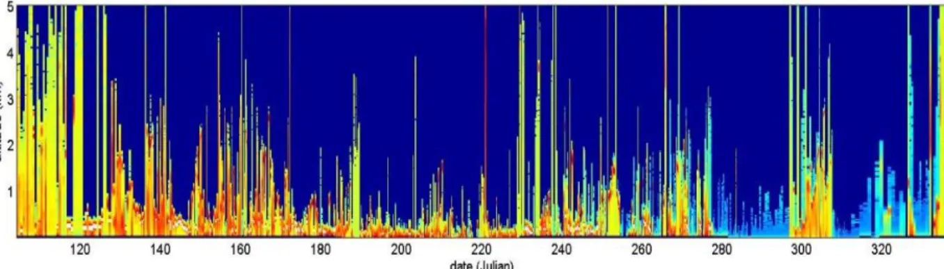
Figure 1: Altitude-time cross-section of the log(PR2) of the whole dataset of 2014 drift. Very low dense clouds, icing of the window and high tilt of the buoy limit most of the time the range of the microlidar.
month period to check calibration on molecular scattering. Results reported in Fig. 2 show no significant drift. The lidar constant is equal to 62 000, in good agreement with estimation from lab measurements and detector data sheet.
Knowing the base and top of clouds (see next section), it is possible to further check the calibration by evaluating the integrated attenuated backscatter signal (usually written as γ) over dense water clouds. This method can provide another estimate of the constant system as the lidar ratio for water cloud is known to be constant or an estimate of multiple scattering knowing the clear air calibration constant [4].
The second arctic drift during the N-ICE 2015 campaign was the opportunity to test the new polarization set up of the microlidar, and to obtain more information on the system. Alignment and calibration using a polarization rotation method to balance parallel and perpendicular signals was performed in lab. From the signal measured on dense liquid water cloud, one can evaluate the multiple scattering
coefficient using the relation
( ) ⁄( ) [5]. A multiple scattering coefficient of 0.81 +/- 0.08 was derived after saturation correction, from test measurements over Paris. This is in good agreement with that found with the similar system from 2014 campaign. System transmission was controlled
and summing up both polarization signals one obtain with this “gamma” method system constants of about 68200 +/- 8900. This is very close (better than 10%) to that obtained with the “molecular method” (73300 +/- 6800) applied to different zones of the total signal for this system.
4. RESULTS
The 2014 drift provided about 750 profiles of total backscattering profiles in the area 80-88°N and 10-25°E. More than one hundred of them were taken at the end of the drift when the window was so iced that absolutely no signal made its way through it. More than fifty percent of the remaining profiles can be considered to be totally or mostly ice- or snow-free, according to the amplitude of the diffused window signal, used as an indicator of window icing.
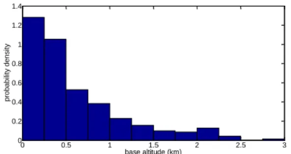
Using Haar wavelet and adapted threshold over vertical profiles, base and effective top of clouds have been retrieved, regardless of how high or low were the amplitude of the window diffused signal. This first analysis shows very low base of clouds (Fig. 3), frequently below1km of altitude and a high frequency of very low (under 1km) altitude cloudiness (as high as 60%), mostly due to supercooled water clouds. This is in good agreement with measurements made during SHEBA [3]. Considering profiles below half the window icing threshold, there are as high as 60% of these profiles showing signal which can be considered as a cloud.
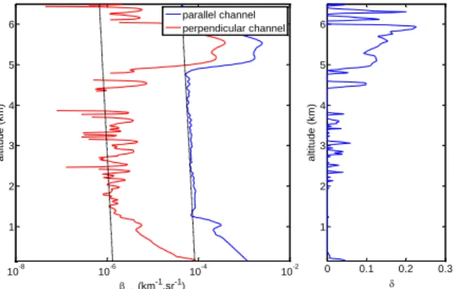
First IAOOS polarized profiles were obtained during N-ICE2015 and normalized with the calibration constant value determined. An example is shown in Figure 4. Depolarization ratio as low as 15-22% are observed, which may mean plate crystals were prevalent [6], although
0 0.5 1 1.5 2 2.5 3 0 0.2 0.4 0.6 0.8 1 1.2 1.4 base altitude (km) p ro b a b ility d e n sity
Figure 3: density of probability of the base altitude of the clouds detected between 0 and 3km.
Figure 2: Values of system constants calculated either on molecular scattering (blue), or on dense water cloud (red) with the “gamma” method and adapted multiple scattering so that good agreement with molecular method was found.
120 140 160 180 200 220 240 260 280 300 320 340 2 3 4 5 6 7 8 9 10 11x 10 4 date (Julian) S yst em con st an t "molecular" method "gamma" method (LR = 19sr-1; = 0.7)
this cloud was at a temperature about –48°C according to data soundings made in Ny-Alesund. The slope below the clouds corresponds to low aerosol contribution superimposed on molecular
scattering. Since the spectral bandwidth transmits only the Cabannes line, one expected about 0.36% of molecular depolarization, instead of the 1.6% observed (ratio between parallel and perpendicular βatt in Fig. 4). This cross-talk effect can be compensated by the previous calibration, and the depolarization ratio in right figure (Fig. 4) does not show this deviation. Depolarized peaks below the clouds are due to the very noisy perpendicular channel signal. Thus at such altitudes one can expect to detect only depolarization above 5%, this threshold increasing with the decrease of SNR. Even if there might be quite high uncertainties for some profiles, the polarization will unambiguously enable the discrimination between liquid water and ice, and help improving our knowledge concerning vertical and temporal cloud structure.
5. CONCLUSIONS
The development of first autonomous microlidar systems developed within the IAOOS project and their first deployment on buoy in the arctic has been successful. Very good first results have been obtained in terms of instrumental unattended operation. New solutions for avoiding icing of the window will be tested. Despite the
icing limitation, valuable statistical analyzes could be started concerning the low level arctic clouds, and therefore IAOOS observations are expected to contribute to a better understanding of radiative budget at the surface, along with ice and ocean measurements simultaneously performed on the buoys by LOCEAN.
ACKNOWLEDGEMENT
We are thankful to the DT/INSU/CNRS for the mechanical and system control design as well as tests of the microlidar and buoy set up in the arctic. We also would like also to thank the Association Nationale de la Recherche et de la Technologie and CIMEL Electronique for supporting the PhD work of V. Mariage, and French Research Ministry EQUIPEX grant for the funding of the IAOOS project.
REFERENCES
[1] Shupe, M. D., J.M. Intrieri, 2004: Cloud radiative forcing of the Arctic surface: The influence of cloud properties, surface albedo, and solar zenith angle, Journal of Climate, 17, 616-628
[2] Wiegner, M., F. Madonna, I. Binietoglou, R. Forkel, J. Gasteiger, A. Geiß, G. Pappalardo, K. Schäfer, W. Thomas, 2014: What is the benefit of ceilometers for aerosol remote sensing? An answer from EARLINET, Atmospheric Measurement Techniques, 7, 2491-2543
[3] Intrieri, J. M., M. D. Shupe, T. Uttal, B. J. McCarty, 2002: An annual cycle of Arctic cloud characteristics observed by radar and lidar at SHEBA, Journal of Geophysical Research: Oceans, 107 (C10),SHE 5-1–SHE 5-15
[4]
O’Connor, E. J., A. J. Illingworth, and R. J. Hogan, 2004: A technique for autocalibration of cloud lidar, J. Atmos. Ocean. Tech., 21, 777-786. [5] Hu, Y., 2007: Depolarization ratio-effective lidar ratio relation: Theoretical basis for space lidar cloud phase discrimination, GeophysicalResearch Letters, 34
[6] Sassen, K., 1991: The polarization lidar technique for cloud research: A review and current assessment, BAMS, 72, 1848-1866.
Figure 4: left: attenuated backscatter coefficient measured in both co- and cross-polarizations during the N-ICE2015 campaign with normalized molecular reference as dashed lines, and right: depolarization ratio obtained with calibration by polarization rotation method after crosstalk correction. All profiles have been filtered over 5 points.
10-8 10-6 10-4 10-2 1 2 3 4 5 6 att (km -1.sr-1) alt it ude (k m ) parallel channel perpendicular channel 0 0.1 0.2 0.3 1 2 3 4 5 6 alt it ude (k m )