Differentiable visual computing

by

Tzu-Mao Li

Submitted to the Department of Electrical Engineering and Computer

Science

in partial fulfillment of the requirements for the degree of

Doctor of Philosophy

at the

MASSACHUSETTS INSTITUTE OF TECHNOLOGY

June 2019

© Massachusetts Institute of Technology 2019. All rights reserved.

Author . . . .

Department of Electrical Engineering and Computer Science

May 10, 2019

Certified by . . . .

Frédo Durand

Professor of Electrical Engineering and Computer Science

Thesis Supervisor

Accepted by . . . .

Leslie A. Kolodziejski

Professor of Electrical Engineering and Computer Science

Chair, Department Committee on Graduate Students

by

Tzu-Mao Li

Submitted to the Department of Electrical Engineering and Computer Science on May 10, 2019, in partial fulfillment of the

requirements for the degree of Doctor of Philosophy

Abstract

Derivatives of computer graphics, image processing, and deep learning algorithms have tremendous use in guiding parameter space searches, or solving inverse problems. As the algorithms become more sophisticated, we no longer only need to differentiate simple mathe-matical functions, but have to deal with general programs which encode complex transfor-mations of data. This dissertation introduces three tools, for addressing the challenges that arise when obtaining and applying the derivatives for complex graphics algorithms.

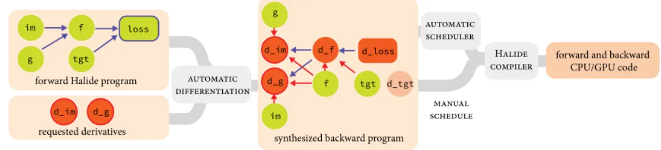
Traditionally, practitioners have been constrained to composing programs with a limited set of coarse-grained operators, or hand-deriving derivatives. We extend the image processing language Halide with reverse-mode automatic differentiation, and the ability to automatically optimize the gradient computations. This enables automatic generation of the gradients of arbitrary Halide programs, at high performance, with little programmer effort. We demon-strate several applications, including how our system enables quality improvements of even traditional, feed-forward image processing algorithms, blurring the distinction between classical and deep learning methods.

In 3D rendering, the gradient is required with respect to variables such as camera pa-rameters, light sources, geometry, and appearance. However, computing the gradient is challenging because the rendering integral includes visibility terms that are not differen-tiable. We introduce, to our knowledge, the first general-purpose differentiable ray tracer that solves the full rendering equation, while correctly taking the geometric discontinuities into account. We show prototype applications in inverse rendering and the generation of adversarial examples for neural networks.

Finally, we demonstrate that the derivatives of light path throughput, especially the second-order ones, can also be useful for guiding sampling in forward rendering. Simulating light transport in the presence of multi-bounce glossy effects and motion in 3D rendering is challenging due to the high-dimensional integrand and narrow high-contribution areas. We extend the Metropolis Light Transport algorithm by adapting to the local shape of the integrand, thereby increasing sampling efficiency. In particular, the Hessian is able to capture the strong anisotropy of the integrand. We use ideas from Hamiltonian Monte Carlo and simulate physics in Taylor expansion to draw samples from high-contribution region. Thesis Supervisor: Frédo Durand

Title: Professor of Electrical Engineering and Computer Science 3

I would like to acknowledge by briefly reflecting how I ended up writing this dissertation. I was fascinated by computer science since I knew the existence of computers. I love the idea of automating tedious computation and the intellectual challenges involved in the process of automation. Naturally, I enrolled in a computer science program during my undergraduate education. At there I was introduced to the enchanting world of computer graphics, where people are able to generate beautiful images with equations and code, instead of pen and paper. During my undergraduate and master’s studies at National Taiwan University, I worked with Yung-Yu Chuang, the professor who brought me into computer graphics research. I started to read academic papers, and was mesmerized by people who contribute their own ideas to improve image generation. In the end I was also able to contribute my own little idea, by publishing a paper related to denoising Monte Carlo rendering images during my Master’s study.

I hoped to do more, and decided to pursue a Ph.D. next. Among all the academic literature I studied, a few names caught my eyes. My Ph.D. advisor Frédo Durand is one of them. His work on frequency analysis for light transport simulation provides a rigorous and insightful theoretical foundation for sampling and reconstruction in light transport. I am also amazed by his versatility in research. At the point this dissertation was written, he has already worked on physically-based rendering, non-photorealistic rendering, computational photography, computer vision, geometric and material modeling, human-computer interaction, medical imaging, and programming systems. After I first met him, I also found out that he has a great sense of humor and is in general a very likable and good-tempered person.

I joined the MIT graphics group as a rendering person. Frédo and I decided that research on Metropolis light transport [216] aligns our interests the most. Metropolis light transport is a classical rendering algorithm that was recently revitalized thanks to Wenzel Jakob’s reimplementation of this notoriously difficult-to-implement algorithm. We found the classical literature of Langevin Monte Carlo [181] and Hamiltonian Monte Carlo [48], and thought that the derivatives information these algorithms use can also help Metropolis light transport. I also learned about the field of automatic differentiation, which later became the most essential tool of this thesis. Frédo, Luke Anderson, and Shuang Zhao had a lot of discussions with me on this topic, which helped to shape my thoughts. Frédo also brought Ravi Ramamoorthi, Jaakko Lehtinen, and Wenzel Jakob into this project. Ravi helped the most on this particular project. When we were collaborating, every week he would monitor my progress, and try to understand the current obstacles and provide advice. While the discussions with Frédo and others are usually higher-level, Ravi tried to understand every single detail of what I

strong influences on my paper writing style. Frédo taught me to focus on the high-level pictures and Ravi taught me to explain everything in a clear manner.

Like many other computer science research projects, this project ended up to be a huge undertaking of software engineering. Our algorithm requires the Hessian and gradient of the light transport contribution. Implementing this efficiently requires complex metaprogram-ming and is very difficult with existing tools. This also motivates my later work on extending the Halide programming language [171] for generating gradients. Nevertheless, I was still able to implement the first differentiable bidirectional path tracer that is able to generate gradient and Hessian of path contribution. We published a paper in 2015.

The results from our first project on improving Metropolis light transport were quite encouraging. This motivated us to look deeper into this subfield. Our derivative-based algorithm helped local exploration, but the bigger issue of these Markov chain Monte Carlo methods lies in the global exploration. As light transport contribution is inherently multi-modal due to discontinuities, the Markov chains in Metropolis light transport algorithms usually have bad mixing. This typically manifests as blotchy artifacts on the images. We were hoping to have a better understanding of the global structure of light transport path space, in order to resolve the exploration issue. Unfortunately, this turns out to be more difficult than we imagined, due to the curse of dimensionality. As the dimensionality of the path space increases, the difficulty to capture the structure increases exponentially. We were able to get decent results by fitting Gaussians on low-dimensional cases (say, 4D), but I got stuck as soon as I proceeded to higher-dimensional space.1

I stuck on the global Metropolis light transport project for nearly two years. In the mean-time, I also explored a few other directions. For example, I tried to generalize gradient domain rendering [127] to the wavelet domain. None of these attempts were very successful. As most researchers already knew, when working on a research project, it is very difficult to know whether the researcher is missing something, or the project simply will go nowhere in the first place. Still, I gained a lot of useful knowledge in these years. During this period, I helped Luke Anderson on his programming system for rendering, Aether [7]. The system stores the Monte Carlo sampling process symbolically, and automatically produces the probability density function of this process. Like my first Metropolis rendering project, this process also heavily involves metaprogramming and huge engineering efforts. This increased my interests in systems research – many computer graphics researches are so engineering heavy,

1_{Recently, Reibold et al. [175] published a similar idea. A key feature that makes their idea works, in my}

opinion, is that they focus on fitting block-tridiagonal covariance matrices for their Gaussian mixtures, instead of the full covariance as we tried. This makes their problem significantly more tractable.

internship at Weta digital to work with the Manuka rendering team, including Marc Droske, Jirí Vorba, Jorge Schwarzhaupt, Luca Fascione. I also met Lingqi Yan, who was also an intern there working on appearance modeling. We often chatted about research and video games together. The internship at Weta taught me a lot about production rendering, visual effects practices, and the beauty of New Zealand.

After I stagnated on the projects for a while, to avoid sunk cost fallacy, Frédo and I decided to temporarily move on. Inspired by the recent success of deep learning, and my frustration on the lack of tools for general and efficient automatic differentiation, we chose to work on automatic differentiating Halide code. We picked Halide because it was developed by our group, so we are sufficiently familiar with it. Halide also strikes the balance between having a more general computation model than most deep learning frameworks, and focused enough for us to optimize the gradient code generation. We contacted Jonathan Ragan-Kelley and Andrew Adams, the parents of Halide, who also had the idea of adding automatic differentiation to Halide for a long time. We also brought in my labmate Michaël Gharbi, who is one of the most knowledgable and likable people in the world, to work on this. I learned a lot about deep learning and data-driven computing from Michaël and a lot about parallel programming systems from Jonathan and Andrew. It was super fun working with these people. I was also happy that my knowledge of automatic differentiation became useful in fields outside of rendering.

At the summer of 2017, I did an internship at Nvidia research at Seattle. Since we published the 2015 paper on improving Metropolis light transport using derivative information, we were always thinking about using it also for inverse rendering. Previous work focused on either simplified model [137] or volumetric scattering [62], and we think there are interesting cases on inverse surface light transport where derivatives can be useful. My collaborator and friend Jaakko saw my internship as an opportunity for pushing me to work in this direction. He also pointed out that the main technical challenge in the surface light transport case would be the non-differentiability. Under the help of Jaakko, Marco Salvi, and Aaron Lefohn, we experimented several different approximation algorithms there. They work well in many cases, but there were always some edge cases that would break the algorithms. The time at Nvidia was a fresh break from graduate school. I met Lingqi again there, and Christoph Peters, another intern who has an unusual passion for the theory of moment reconstruction problems, and always have only apples for his lunch. I also met two other interns Qi Sun, Tri Nguyen and maintained friendships with them since then.

After I wrapped up my internship at Nvidia and returned to MIT, I and Jaakko talked with Frédo and Miika Aittala about the inverse rendering project. Frédo pointed out the relation

between the mesh discontinuities and silhouette rasterization [190]. After more discussions, we realized that this is highly related to Ravi’s first-order analysis work back in 2007 [173]. I worked out the math and generalized Ravi’s theory to arbitrary parameters, primary visibility, and global illumination. Based on my experience on the differentiable bidirectional path tracer from 2015, I was able to quickly come up with a prototype renderer and to write a paper about this.

This is how this dissertation was written.

Since I mostly focused on the research part of the story, many people were left out. I am grateful to the labmates in MIT graphics group. Lukas Murmann and Alexandre Kaspar were the students who joined the group at the same time as me. Naturally, we hung out a lot together (by my standard). YiChang Shih, Abe Davis, and Valentina Shin are the senior students who guided us when we were lost. Zoya Bylinski made sure we always have enough snacks and coffee in the office. I enjoyed all the trash-talks with Tiam Jaroensri. Prafull Sharma’s jokes are sometimes funny, sometimes not too much. Camille Biscarrat and Caroline Chan brought energy and fresh air to our offices. I had a lot of nerdy programming languages chat with Yuanming Hu. It was also fun to chat about research with Gaurav Chaurasia, Aleksandar Zlateski, and David Levin. Luke Anderson proofread every single paper I have written, including this dissertation. Nathaniel Jones broadened my view on rendering’s application in architectural visualization.

The reviewer #1 of the inverse rendering paper, who I suspect to be Ravi, provided an extremely detailed and helpful review. My thesis committee Justin Solomon and Wojciech Matusik also provided useful comments. Justin pointed out the relation between the Reynold transport theorem and our edge sampling method in the inverse rendering project. I should also thank NSF and Toyota Research Institute for the funding support, so I don’t freeze to death in Boston.

Anton Kaplanyan invited me to intern at Facebook Reality Lab during 2018. I met Thomas Leimkühler, Steve Bako, Christoph Schied, and Michael Doggett there. FRL was a very competitive and vigorous environment. I loved the free food. They had smoked salmon for the breakfast! I worked with Dejan Azinović, Matthias, Nießner and Anton there on a material and lighting reconstruction project.

I met my girlfriend Ailin Deng at the end of 2017. She has since then become the oasis that shelters me when I am tired of programming and research. I thank I-Chao Shen and Sheng-Chieh Chin for being patient for listening to my rants and non-sensical research ideas. I am grateful that my parents remain supportive throughout my studies on computer science.

1 Introduction 13

1.1 Background and Target Audience . . . 17

1.2 Publications . . . 17

2 Automatic Differentiation 19 2.1 Finite Differences and Symbolic Derivatives . . . 20

2.2 Algorithms for Generating Derivatives . . . 21

2.2.1 Forward-mode . . . 23

2.2.2 Reverse-mode . . . 25

2.2.3 Beyond Forward and Reverse Modes . . . 27

2.3 Automatic Differentiation as Program Transformation . . . 27

2.3.1 Control Flow and Recursion . . . 29

2.4 Historical Remarks . . . 31

2.5 Further Readings . . . 32

3 Derivative-based Optimization and Markov Chain Monte Carlo Sampling 35 3.1 Optimization . . . 35

3.1.1 Gradient Descent . . . 36

3.1.2 Stochastic Gradient Descent . . . 37

3.1.3 Newton’s Method . . . 38

3.1.4 Adaptive Gradient Methods . . . 39

3.2 Markov Chain Monte Carlo Sampling . . . 41

3.2.1 Metropolis-Hastings Algorithm . . . 42

3.2.2 Langevin Monte Carlo . . . 44

3.2.3 Hamiltonian Monte Carlo . . . 45

3.2.4 Stochastic Langevin or Hamiltonian Monte Carlo . . . 46

3.3 Relation between Optimization and Sampling . . . 46 9

4 Differentiable Image Processing and Deep Learning in Halide 49

4.1 Related Work . . . 53

4.1.1 Automatic Differentiation and Deep Learning Frameworks . . . 53

4.1.2 Image Processing Languages . . . 53

4.1.3 Learning and Optimizing with Images . . . 54

4.2 The Halide Programming Language . . . 54

4.3 Method . . . 56

4.3.1 High-level Strategy . . . 56

4.3.2 Differentiating Halide Function Calls . . . 57

4.3.3 Checkpointing . . . 61

4.3.4 Automatic Scheduling . . . 63

4.4 Applications and Results . . . 64

4.4.1 Custom Neural Network Layers . . . 64

4.4.2 Parameter Optimization for Image Processing Pipelines . . . 67

4.4.3 Inverse Imaging Problems: Optimizing for the Image . . . 71

4.4.4 Non-image-processing Applications . . . 72

4.4.5 Future Work . . . 73

4.5 Conclusion . . . 74

5 Differentiable Monte Carlo Ray Tracing through Edge Sampling 75 5.1 Related Work . . . 76 5.1.1 Inverse Graphics . . . 76 5.1.2 Derivatives in Rendering . . . 77 5.2 Method . . . 78 5.2.1 Primary Visibility . . . 79 5.2.2 Secondary visibility . . . 84

5.2.3 Cameras with Non-linear Projections . . . 86

5.2.4 Relation to Reynolds transport theorem and shape optimization . . . 87

5.3 Importance Sampling the Edges . . . 87

5.3.1 Edge selection . . . 89

5.3.2 Importance sampling on an edge . . . 90

5.3.3 Next event estimation for edges . . . 90

5.4 Results . . . 91

5.4.1 Verification of the method . . . 92

5.4.2 Comparison with previous differentiable renderers . . . 94

5.4.4 Inverse rendering application . . . 95

5.4.5 3D adversarial example . . . 96

5.4.6 Limitations . . . 96

5.5 Conclusion . . . 98

5.A Derivation of the 3D edge Jacobian . . . 98

6 Hessian-Hamiltonian Monte Carlo Rendering 101 6.1 Related Work . . . 104

6.2 Hamiltonian Monte Carlo . . . 107

6.3 Hessian-Hamiltonian Monte Carlo . . . 111

6.4 Implementation . . . 118

6.5 Results and Discussion . . . 120

6.5.1 Limitations and Future Work . . . 122

6.6 Conclusion . . . 123

6.A Pseudo-code for H2_{MC . . . 123}

Differential calculus seeks to characterize the local geometry of a function. By definition, the derivatives at a point of a function tell us what happens to the outputs if we slightly move the point. This property enables us to make smarter decisions, and makes derivatives a fundamental tool for various tasks including parameter tuning, solving inverse problems, and sampling.

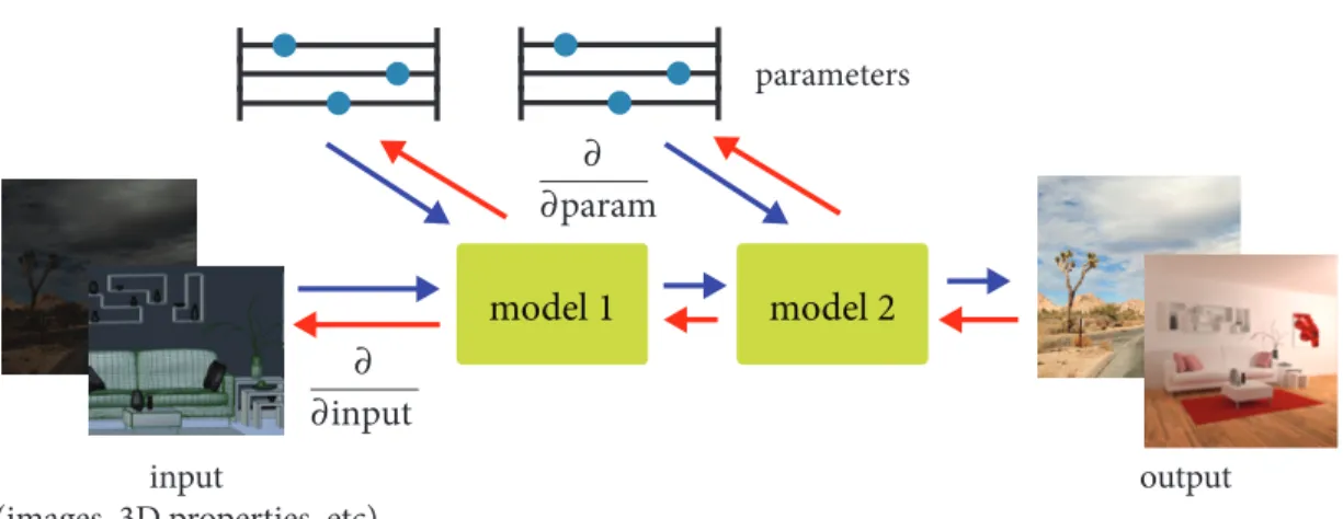
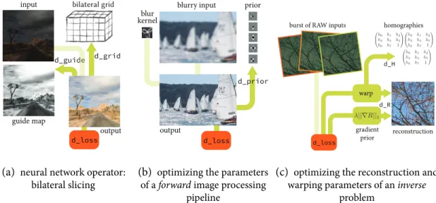
As computer graphics and image processing algorithms become more sophisticated, computing derivatives for functions defined in these algorithms becomes more important. Derivatives are useful in both data-driven and non data-driven scenarios. For one thing, as the number of parameters of the algorithm increases, it becomes infeasible to manually adjust them to achieve the desired behavior. Data-driven approaches allow us to automatically tune the parameters of our model. For another thing, these sophisticated forward models can be used for solving inverse problems. For example, the computer graphics community has developed mature models of how photons interact with scenes and cameras, and it is desirable to incorporate this knowledge, instead of learning it from scratch using a data-driven approach. Finally, differentiable algorithms are composable, which means we can piece different differentiable algorithms together, and have an end-to-end differentiable system as a whole. This enables us to compose novel algorithms by adding other differentiable components to the pipeline, such as deep learning architectures. Figure 1-1 illustrates the use of derivatives.

While deep learning has popularized the use of gradient-based optimization over highly-parameterized functions, the current building blocks used in deep learning methods are very limited. A typical deep learning architecture is usually composed of convolution filters, linear combinations of elements (“fully connected” layer), subsampling by an integer factor (“pooling”, usually by a factor of 2), and element-wise nonlinearities. Most visual computing algorithms are far more sophisticated than these. They often combine neighboring pixels using non-linear kernels (e.g. [209, 28]), downsample a signal prefiltered by some antialiasing filters (e.g. [150]), use heavy-tailed non-linear functions to model the reflectance of surfaces (e.g. [43]), or traverse trees for finding intersections between objects (e.g. [40]).

input

(images, 3D properties, etc) output

parameters model 1 model 2 ∂ ∂input ∂ ∂param

Figure 1-1: Differentiable visual computing. Derivatives enable us to make smart decisions in our models. The derivatives of a model’s output can be taken with respect to the parameters or the inputs of the model. This makes it possible to find corresponding inputs for a given output, solving an inverse problem, or we can find model parameters that map inputs to outputs. This is useful in both data-driven and non-data-driven applications.

I argue that most numerical algorithms in computer graphics and image processing should be implemented in a differentiable manner. This is beneficial for both data-driven and non-data-driven applications. Comparing to deep learning approaches, this allows better control and interpretability by integrating the domain knowledge into the model. It makes debugging models a lot easier since we have a better idea of how data should interact with the model. It is often more efficient both in time and memory, and more accurate, since the model is more tailored to the applications.

Efficiently evaluating derivatives from algorithms that perform complex transformations on 3D data or 2D images presents challenges in both systems and algorithms. Firstly, existing deep learning frameworks (e.g. [1, 165]) only have limited expressiveness. While automatic differentiation methods (e.g. [71]) can generate derivatives from almost arbitrary algorithms, generating efficient derivative code while taking parallelism and locality into consideration is still difficult. Secondly, the algorithms can introduce discontinuities. For example, in 3D rendering, the visibility term is discontinuous, which prevents direct application of automatic differentiation. Finally, designing algorithms that efficiently utilize the obtained derivatives is also important.

The contributions of this dissertation are three novel tools for addressing the challenges and for investigating the use of derivatives in the context of visual computing.

Efficient Automatic Differentiation for Image Processing and Deep Learning In

Chap-ter 4, we address the systems challenges for efficiently generating derivatives code from image processing algorithms. Existing tools for automatically generating derivatives have at least one of the following two issues:

• General automatic differentiation systems (e.g. [22, 69, 77, 86, 229]) are inefficient because they do not take parallelism and locality into consideration.

• Deep learning frameworks (e.g. [1, 165]) are inflexible because they are composed of coarse-grained, specialized operators, such as convolutions or element-wise operations. For many applications, it is often difficult to assemble these operators to build the desired algorithm. Even when done successfully, the resulting code is often both slow and memory-inefficient, saving and reloading entire arrays of intermediate results between each step, causing costly cache misses.

These limitations are one of the main obstacles preventing researchers and developers from inventing novel differentiable algorithms, since they are often required to manually derive and implement the derivatives in lower-level languages such as C++ or CUDA.

In this chapter, we focus on image processing and deep learning. We build on the image processing language Halide [171, 172], and extend it with the ability to generate gradient code. Halide provides a concise and natural language for expressing image processing algorithms, while allowing the separation between high-level algorithm and low-level scheduling for achieving high-performance across platforms. To generate efficient gradient code, we develop a compiler transformation for generating gradient code automatically from Halide algorithms. Keys to making the transformation work are a scatter-to-gather conversion algorithm which preserves parallelism, and a simple automatic scheduling algorithm which specializes in the patterns in gradient code and provides a GPU backend.

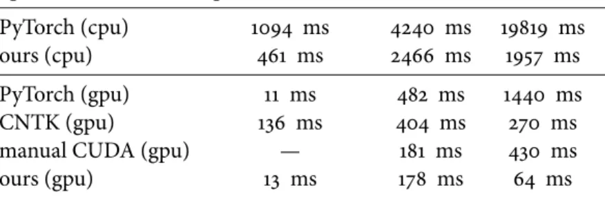
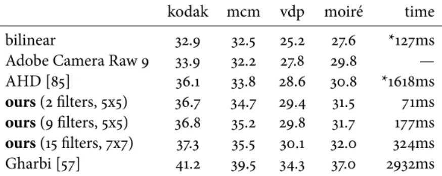
Using this new extension of Halide, we show first that we can concisely and efficiently implement existing custom deep learning operators, which previously required implementa-tion in low-level CUDA. Our generated code is as fast or even faster than the corresponding high-performance hand-written code, with less than 1⇑10 of the lines of code. Secondly, we show that gradient-based parameter optimization is useful outside of traditional deep learn-ing approaches. We significantly improve the accuracy of two traditional image processlearn-ing algorithms by augmenting their parameters and automatically optimizing them. Thirdly, we show that the system is also useful for inverse problems. We implement a novel joint burst demosaicking and superresolution algorithm by building a forward image formation model. Finally, we demonstrate our extension’s versatility by implementing two applications

outside of image processing – lens design optimization through a ray tracer and a classical fluid simulator in computer graphics [201].

Differentiable Monte Carlo Ray Tracing through Edge Sampling While automatic

dif-ferentiation generates derivatives, it does not handle non-differentiability in individual code paths. In particular, for computer graphics, we are interested in the gradients of the 3D rendering operation with respect to variables such as camera parameters, light sources, scene geometry, and appearance. While the rendering integral is differentiable, the integrand is discontinuous due to visibility. Previous works on differentiable rendering (e.g. [137, 109]) focused on fast approximate solutions, and do not handle secondary effects such as shadows or global illumination.

In Chapter 5, we introduce a general-purpose differentiable ray tracer, which, to our knowledge, is the first comprehensive solution that is able to compute the gradients of the rendering integral with respect to scene parameters, while correctly taking geometric discontinuities into consideration. We observe that the discontinuities in the rendering integral become Dirac delta functions when taking the gradient. Therefore we develop a novel method for explicit sampling of the triangle edges that introduce the discontinuities. This requires new spatial acceleration techniques and importance sampling for efficiently selecting edges.

We integrate our differentiable ray tracer with the automatic differentiation library Py-Torch [165], and demonstrate prototype applications for inverse rendering and finding adver-sarial examples for neural networks.

Hessian-Hamiltonian Monte Carlo Rendering Finally, we show that derivatives,

espe-cially the second-order ones, can also be used for accelerating forward rendering by guiding light path sampling. In Chapter 6, we present a Markov chain Monte Carlo rendering al-gorithm that automatically and explicitly adapts to the local shape of the integrand using the second-order Taylor expansion, thereby increasing sampling efficiency. In particular, the Hessian is able to capture the strong anisotropy caused by challenging effects such as multi-bounce glossy effects and motion.

Using derivatives in the context of sampling instead of optimization requires more care. The second-order Taylor expansion does not define a proper distribution, and therefore cannot be directly importance sampled. We use ideas from Hamiltonian Monte Carlo [48] that simulates Hamiltonian dynamics in a flipped version of the Taylor expansion where gravity pulls particles towards the high-contribution region. The quadratic landscape leads to a closed-form anisotropic Gaussian distribution, and results in a standard

Metropolis-Hastings algorithm [78].

Unlike previous works that derive the sampling procedures manually and only consider specific effects, our resulting algorithm is general thanks to automatic differentiation. In particular, our method is the first Markov chain Monte Carlo rendering algorithm that is able to resolve the anisotropy in the time dimension and render difficult moving caustics.

1.1 Background and Target Audience

Chapter 2 and Chapter 3 review the background of automatic differentiation, optimization, and sampling, and their relationship. These are not novel components of this dissertation, but they represent important components that are glossed over in the individual publications. Moreover, they connect the central themes of this dissertation: differentiating algorithms and making use of the resulting derivatives.

I imagine the majority of readers of this dissertation to be researchers in the fields of computer graphics, image processing, systems or machine learning, who are interested in using the individual tools and want to know the details better, or people who are building their own differentiable systems. For both groups of people, I hope the examples in this dissertation can improve your intuition on building differentiable systems in the future.

1.2 Publications

The content of this dissertation has appeared in the following publications:

• Chapter 4: Tzu-Mao Li, Michaël Gharbi, Andrew Adams, Frédo Durand, and Jonathan Ragan-Kelley. Differentiable programming for image processing and deep learning in Halide. ACM Trans. Graph. (Proc. SIGGRAPH), 37(4):139:1–139:13, 2018

• Chapter 5 Tzu-Mao Li, Miika Aittala, Frédo Durand, and Jaakko Lehtinen. Differ-entiable Monte Carlo ray tracing through edge sampling. ACM Trans. Graph. (Proc. SIGGRAPH Asia), 37(6):222:1–222:11, 2018

• Chapter 6 Tzu-Mao Li, Jaakko Lehtinen, Ravi Ramamoorthi, Wenzel Jakob, and Frédo Durand. Anisotropic Gaussian mutations for Metropolis light transport through Hessian-Hamiltonian dynamics. ACM Transactions on Graphics (Proc. SIGGRAPH Asia), 34(6):209:1–209:13, 2015

The source code of the projects can be downloaded from the corresponding project sites: • http://gradients.halide-lang.org/

• https://people.csail.mit.edu/tzumao/diffrt/ • https://people.csail.mit.edu/tzumao/h2mc/

For Chapter 4, I added a hindsight on differentiating scan operations (Chapter 4.3.2) and an example of fluid simulation (Chapter 4.4.4) since the publication.

For Chapter 5, I added more discussions about the pathelogical parallel edges condition where our method can produce incorrect result (Chapter 5.2). There is also some discus-sions regarding non-linear camera models (Chapter 5.2). I added some discussion related to Reynolds transport theorem and shape optimization (Chapter 5.2.4). I also revised the edge selection algorithm (Chapter 5.3.1), added some discussions about a GPU implementa-tion (Chapter 5.4), and added discussions about differentiable geometry buffer rendering (Chapter 5.4.3).

For Chapter 6, I added a description of an improved large step mutation method (Chap-ter 6.4), and some discussions to recent works (Chap(Chap-ter 6.5.1).

Evaluating derivatives for computer graphics and image processing algorithms is the key to this dissertation. We will use them to minimize cost functions, solve inverse problems, and guide sampling procedures. Intuitively speaking, the derivatives of a function characterize the local behavior at a given point, e.g. if I move the point to this direction, will the output values become larger or smaller? This allows us to find points that result in certain function values, such as maximizing a utility function, or minimizing the difference between the output and a target.

In this chapter, we review the methods for generating derivatives from numerical pro-grams. The chapter serves as an introductory article to the theory and practice of automatic differentiation. The reader is encouraged to read Griewank and Walther’s textbook [71] for a comprehensive treatment of the topic.

Given a computer program containing control flow, loops, and/or recursion, with some real number inputs and some real number outputs, our goal is to compute the derivatives between the outputs and the inputs. Sometimes there is only a scalar output but more than one input, in which case we are interested in the gradient vector. Sometimes there are multiple outputs as well, and we are interested in the Jacobian matrix. Sometimes we are interested in the higher-order derivatives such as the Hessian matrix.

While the title of this chapter is automatic differentiation, we will also talk about how to differentiate a program manually, which is less difficult than one might imagine. We show how to systematically write down the derivative code just by looking at a program, without lengthy and convoluted mathematical notation. While this is still more tedious and error-prone than an automatic compiler transformation (which is why we develop the tool in Chapter 4), it is a useful practice for understanding the structure of derivative code, and is even practical sometimes if it is difficult to parse and transform the code.

2.1 Finite Differences and Symbolic Derivatives

Before discussing automatic differentiation algorithms, it is useful to review other ways of generating derivatives, and compare them to automatic differentiation.

A common approximation for derivatives are finite differences, sometimes also called numerical derivatives. Given a function f (x) and an input x, we approximate the derivative by perturbing x by a small amount h:

d f_(x) dx ≈ f_{(x + h) − f (x)} h or (2.1) d f_(x) dx ≈ f_{(x + h) − f (x − h)} 2h . (2.2)

The problem with this approximation is two-fold. First, the optimal choice of the step size h in a computer system is problem dependent. If the step size is too small, the rounding error of the floating point representation becomes too large. On the other hand, if the step size is too large, the result becomes a poor approximation to the true derivative. Second, the method is inefficient for multivariate functions. For a function with 100 variables and a scalar output, computing the full gradient vector requires at least 101 evaluations of the original function.

Another alternative is to treat the content of the function f as a sequence of mathemat-ical operations, and symbolmathemat-ically differentiate the function. Indeed, most of the rules for differentiation are mechanical, and we can apply the rules to generate f′(x). However, in our

case, f (x) is usually an algorithm, and symbolic differentiation does not scale well with the number of symbols. Consider the following code:

function f(x): result = x

for i = 1 to 8:

result = exp(result)

return result

Figure 2-1: A code example that iteratively computes a nested exponential for demonstrating the difference between symbolic differentiation and automatic differentiation.

Using the symbolic differentiation tools from mathematical software such as Mathemat-ica [93] would result in the following expression:

d f_(x) dx = e x+eee ee ee x +ee ee ee x +ee ee ex +ee ee x +ee ex +ee x +ex. (2.3)

much larger. Using forward-mode automatic differentiation, which will be introduced later, we can generate the following code for computing derivatives:

function d_f(x): result = x d_result = 1

for i = 1 to 8:

result = exp(result)

d_result = d_result * result

return d_result

The code above outputs the exact same values as the symbolic derivative (Equation 2.3), but is significantly more efficient (8 v.s. 37 exponentials). This is due to automatic differentiation’s better use of the intermediate values and the careful factorization of common subexpressions.

2.2 Algorithms for Generating Derivatives

For a better understanding of automatic differentiation, before introducing the fully auto-matic solution, we will first discuss how to manually differentiate a code example. We start from programs with only function calls and elementary operations such as addition and multiplication. In particular, we do not allow recursive or circular function calls. Later in Chapter 2.3.1, we generalize the idea to handle control flow such as loops and branches, and handle recursion. Throughout the chapter, we assume all function calls are side-effect free. To the author’s knowledge, there are no known automatic differentiation algorithms for transforming arbitrary functions with side effects.

The key to automatic differentiation is the chain rule. Consider the following code with inputxand outputz:

y = f(x) z = g(y)

Assume we already know the derivative functions d f (x) dx and

d g(y)

d y , and we are interested

in the derivative of the outputzwith respect to inputx. We can compute the derivative by

applying the chain rule:

dydx = dfdx(x) dzdy = dgdy(y) dzdx = dzdy * dydx

We can recursively apply the rule to generate derivative functions, until the function is an elementary function for which we know the analytical derivatives, such as addition, multiplication,sin(), orexp().

A useful mental model for automatic differentiation is the computational graph. It can be used for representing dependencies between variables. The nodes of the graph are the variables and the edges are the derivatives between the adjacent vertices. In the case above the graph is linear:

x y z

d y dx

dz d y

Computing derivatives from a computational graph involves traversal of the graph, and gathering of different paths that connect inputs and outputs.

In practice, most functions are multivariate, and often times we want to have multiple derivatives such as for the gradient vector. In this case, different derivatives may have common paths in the computational graph that can be factored out, which can greatly impact efficiency. Consider the following code example and its computational graph:

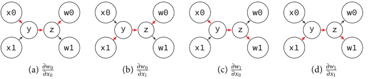
y = f(x0, x1) z = g(y) w0, w1 = h(z) x0 x1 y z w0 w1

Figure 2-2: Code example and computational graph with two inputsx0, x1and two outputsw0, w1

There are four derivatives between the two outputs and two inputs. We can obtain them by traversing the four corresponding paths in the computational graph:

x0 x1 y z w0 w1 (a)∂w₀ ∂x₀ x0 x1 y z w0 w1 (b)∂w₀ ∂x₁ x0 x1 y z w0 w1 (c) ∂w₁ ∂x₀ x0 x1 y z w0 w1 (d)∂w₁ ∂x₁

For example, in (a), the derivative ofw0with respect tox0is the product of the three red

edges: ∂w₀ ∂x₀ = ∂w₀ ∂z ∂z ∂ y ∂ y ∂x₀, (2.4)

and in (b), the derivative ofw0with respect tox1is ∂w₀ ∂x₁ = ∂w₀ ∂z ∂z ∂ y ∂ y ∂x₁. (2.5)

We can observe that some of the derivatives share common subpaths in the computational graph. For example the two derivatives above ∂w₀

∂x₀ and ∂w₀

∂x₁ share the same subpathy, z,

w0. We can therefore factor this subpath out and premultiply ∂w_{∂ y}0 = ∂w_∂z0_{∂ y}∂z for the two

derivatives. In a larger computational graph, this factorization can have enormous impact on the performance of the derivative code, even affecting the time complexity in terms of the number of inputs or outputs.

Different automatic differentiation algorithms find common factors in the computational graph in different ways. In the most general case, finding a factorization that results in minimal operations is NP-hard [154]. Fortunately, in many common cases, such as factorization for the gradient vector, there are efficient solutions.1

If the input is a scalar variable, no matter how many variables there are in the output, forward-modeautomatic differentiation generates derivative code that has the same time complexity as the original algorithm. On the other hand, if the output is a scalar variable, no matter how many input variables there are, reverse-mode automatic differentiation generates derivative code that has the same time complexity as the original algorithm. The latter case is particularly interesting, since it means that we can compute the gradient with the same time complexity (the “cheap gradient principle”), which can be useful for various optimization and sampling algorithms.

Next, we demonstrate several algorithms for computing the derivatives while carefully tak-ing the common subexpressions into consideration. We show how to transform a numerical algorithm with control flow, loops, or recursion to code that generates the derivatives.

2.2.1 Forward-mode

We start with the simplest algorithm, usually called forward-mode automatic differentiation, and sometimes also called dual number (see Chapter 2.4 for historical remarks). Forward-mode traverses the computational graph from the inputs to outputs, computing derivatives of the intermediate nodes with respect to all input variables along the way. Forward-mode is efficient when the input dimension is low and the output dimension is high, since for each node in the computational graph, we need to compute the derivatives with respect to every single input variable.

1_{However, this does not take parallelism and memory efficiency into consideration. We show in Chapter 4}

In computer graphics, forward-mode has been used for computing screen-space deriva-tives for texture prefiltering in 3D rendering [90, 118], for computing derivaderiva-tives in differential equations for physical simulation [72], and for estimating motion in specular objects [243]. Forward-mode is also useful for computing the Hessian, where one can first apply forward-mode then apply reverse-forward-mode on each output to obtain the full Hessian matrix.

We will describe forward-mode using the previous example in Figure 2-2. Starting from the inputs, the goal is to propagate the derivatives with respect to the inputs using the chain rule. To handle function calls, for every functionf(x)referenced by the output variables, we

generate a derivative functiondf(x, dx), wheredxis the derivative ofxwith respect to the

input variables.

We start from the inputsx0, x1and generate ∂x_∂x0

0 =1 and ∂x₁

∂x₁ =1. We use a 2D vector

dx0dxto represent the derivatives ofx0with respect tox0andx1.

dx0dx = {1, 0} dx1dx = {0, 1} y = f(x0, x1) z = g(y) w0, w1 = h(z) x0 x1 y z w0 w1

We then obtain the derivatives forywith respect to the inputs. We assume we already

applied forward-mode automatic differentiation forf, so we have a derivative function df(x0, dx0dx, x1, dx1dx). dx0dx = {1, 0} dx1dx = {0, 1} y = f(x0, x1) dydx = df(x0, dx0dx, x1, dx1dx) z = g(y) w0, w1 = h(z) x0 x1 y z w0 w1

We then propagate the derivative toz: dx0dx = {1, 0} dx1dx = {0, 1} y = f(x0, x1) dydx = df(x0, dx0dx, x1, dx1dx) z = g(y) dzdx = dg(y, dydx) w0, w1 = h(z) x0 x1 y z w0 w1

Finally, we propagate the derivatives fromzto the outputsw0, w1. dx0dx = {1, 0} dx1dx = {0, 1} y = f(x0, x1) dydx = df(x0, dx0dx, x1, dx1dx) z = g(y) dzdx = dg(y, dydx) w0, w1 = h(z) dw0dx, dw1dx = dh(z, dzdx) x0 x1 y z w0 w1

The time complexity of the code generated by forward-mode automatic differentiation is O_(d)times the time complexity of the original algorithm, where d is the number of input variables. It is efficient for functions with few input variables.

However, for many applications of derivatives, we need to differentiate functions with thousands or even millions of input variables. Using forward-mode for this would be infeasi-ble, as we need to compute the derivatives with respect to all input variables for every output in the computational graph. Fortunately, there is another algorithm called reverse-mode automatic differentiation that can generate derivative code that has the same time complexity as the original algorithm when there is only a single output, regardless of the number of input variables.

2.2.2 Reverse-mode

Reverse-mode propagates the derivatives from outputs to inputs, unlike forward-mode, which propagates the derivatives from inputs to outputs. For each node in the computational graph, we compute the derivatives of all outputs with respect to the variable at that node. Therefore reverse-mode is much more efficient when the input dimension is large and the output dimension is low. However, reverse-mode is also more complicated to implement since it needs to run the original algorithm backward to propagate the derivatives.

We again use the same previous example in Figure 2-2 to illustrate how reverse-mode works. Similar to forward-mode, we need to handle function calls. For every functiony = f (x)referenced by the output variables, we generate a derivative functiondf(x, dy), where

d y is a vector of derivatives of the final output with respect to the function’s output_y(in contrast, in forward-mode, the derivative functions take the input derivatives as arguments). Handling control flow and recursion in reverse-mode is more complicated. We discuss them in Chapter 2.3.1.

We start from the outputsw0, w1using ∂w_∂w0

0 =1 and ∂w₁

∂w₁ =1. We use a 2D vectordwdw0to

represent the derivatives ofw0, w1with respect tow0. y = f(x0, x1) z = g(y) w0, w1 = h(z) dwdw0 = {1, 0} dwdw1 = {0, 1} x0 x1 y z w0 w1

Next, we propagate the derivatives to variablezon which the two outputs depend. We

assume we already applied reverse-mode to the functionhand havedh(z, dwdw0, dwdw1). y = f(x0, x1) z = g(y) w0, w1 = h(z) dwdw0 = {1, 0} dwdw1 = {0, 1} dwdz = dh(z, dwdw0, dwdw1) x0 x1 y z w0 w1

Similarly, we propagate toyfromz. y = f(x0, x1) z = g(y) w0, w1 = h(z) dwdw0 = {1, 0} dwdw1 = {0, 1} dwdz = dh(z, dwdw0, dwdw1) dwdy = dg(y, dwdz) x0 x1 y z w0 w1

Finally we obtain the derivatives of the outputswwith respect to the two inputs. y = f(x0, x1) z = g(y) w0, w1 = h(z) dwdw0 = {1, 0} dwdw1 = {0, 1} dwdz = dh(z, dwdw0, dwdw1) dwdy = dg(y, dwdz) dwx0, dwx1 = df(x0, x1, dwdy) x0 x1 y z w0 w1

A major difference between reverse-mode and forward-mode that makes the implementa-tion of reverse-mode much more complicated, is that we can only start the differentiaimplementa-tion after the final output is computed. This makes it impossible to interleave the derivative code with the original code like in forward-mode. This issue has the most impact when differentiating programs with control flow or recursion. We discuss them in Chapter 2.3.1.

2.2.3 Beyond Forward and Reverse Modes

As we have discussed, forward-mode is efficient when the number of inputs is small, while reverse-mode is efficient when the number of outputs is small. When both the number of inputs and the number of outputs are large, and we are interested in the Jacobian or its subset, both forward and reverse modes can be inefficient.

In general, we can think of derivative computation as a pathfinding problem on the computational graph: We want to find all the paths that connect between inputs and outputs. Many of the paths share common subpaths and it is more computationally efficient to factor out the common subpaths. Forward-mode and reverse-mode are two different greedy ap-proaches that factor out the common subpaths either from the input node or output node, and they can deliver suboptimal results that do not have the minimal amount of computation. For the general Jacobian, finding the factorization that results in the minimal amount of computation is called the “Jacobian accumulation problem” and is proven to be NP-Hard [154]. However, there exist several heuristics (e.g. [70, 153, 73]). Usually, the heuristics use some form of a greedy approach to factor the node that is reused by the most paths. These heuristics can also be used for higher-order derivatives such as Hessian matrices [65, 223], since the Hessian is the Jacobian of the gradient vector with respect to the input dimensions.

2.3 Automatic Differentiation as Program Transformation

In this section, we discuss the practical implementation of automatic differentiation. Typically the implementation of automatic differentiation systems can be categorized as a point in a spectrum, depending on how much is done at compile-time. At one end of the spectrum, the tracing approach, or sometimes called the taping approach, re-compiles the derivatives whenever we evaluate the function. At the other end of the spectrum, the source transforma-tionapproach does as much at compile-time as possible by compiling the derivative code only once. The tracing approach has the benefit of simpler implementation, and is easier to incorporate into existing code, while the source transformation approach has better perfor-mance, but usually can only handle a subset of a general-purpose language and is much more

difficult to implement.

Tracing The tracing approach bears similarity to the tracing just-in-time compilation

tech-nique used by various interpreters. Tracing automatic differentiation usually records a linear sequence of the computation at run-time (usually called a tape or Wengert list [227]). Typ-ically, all the control flows will be flattened in the trace. The system then “compiles” the derivatives just-in-time by traversing the linear sequence. A typical implementation is to use operator overloading on a special floating point type, replacing all the elementary operations by the overloaded functions. The user is then required to replace all the floating point type occurences with the special type in their program, and call a compile function to start the differentiation.

Tracing is the most popular method for implementing general automatic differentiation systems. Most of the popular automatic differentiation systems use tracing (e.g. CppAD [16], ADOL-C [69], Adept [86], and Stan [207]). However, tracing is inefficient due to the limited amount of work that can be done during the just-in-time differentiation. For example, if a function is linear, all of the derivatives of it are constant, however, tracing approaches often fail to perform constant folding optimization, since folding the constant at run-time is often more costly than just computing the constant. Metaprogramming techniques such as expression templates can help mitigate this issue [86, 188], but they cannot optimize across functions or even statements.

Source Transformation Another approach is to take the source code of some numerical

program, and generate the code for the derivatives. It is also possible to build an abstract syntax tree using operator overloading, then generate derivative code from the tree (the systems in Chapter 4 and Chapter 5 used precisely this approach). This approach is much more efficient compared to tracing due to the number of optimizations that can be done at compile-time (constant folding, copy elision, common subexpression elimination, etc). However, it is more difficult to integrate into existing languages, and often can only handle a subset of the language features. For example, none of the existing source transformation methods is able to handle functions with arbitrary side effects.

In Chapter 2.2 we already discussed general rules for handling elementary operations and function calls. A straightforward line to line syntax tree transformation should do the job. In the subsection below, we briefly discuss how source transformation can be done for programs with control flow including for loops and while loops, and how to handle recursion or cyclic function calls.

2.3.1 Control Flow and Recursion

Handling control flow and recursion in forward-mode is trivial. We do not need to modify the flow at all. Since forward-mode propagates from the inputs, for each statement, we can compute its derivative immediately after like we did in Chapter 2.2.1.

In reverse-mode, however, control flow and recursion introduce challenges, since we need to revert the flow. Consider the iterative exponential example from Figure 2-1. To apply reverse-mode, we need to revert the for loop. We observe an issue here: we need the intermediateexp(result)values for the derivatives. To resolve this, we will need to record

the intermediate values during the first pass of the loop:

function d_f(x): result = x results = [] for i = 1 to 8: results.push(result) result = exp(result) d_result = 1 for i = 8 to 1: // one-based indexing

d_result = d_result * exp(results[i])

return d_result

The general strategy for transforming loops in reverse-mode is to push intermediate variables into a stack for each loop [217], then pop the items during the reverse loop. Nested loops can be handled in the same way. For efficient code generation, dependency analysis is often required to push only variables that will be used later to the stack (e.g. [202]).

The same strategy of storing intermediate variables in a stack also works for loop con-tinuations, early exits, and conditioned while loops. We can use the size of the stack as the termination criteria. For example, we modify the previous example to a while loop and highlight the derivative code in red:

function d_f(x): result = x

results = []

while result > 0.1 and result < 10:

results.push(result)

result = exp(result)

d_result = 1

for i = len(results) to 1:

d_result = d_result * exp(results[i])

return d_result

Recursion is equally or even more troublesome compared to control flow for reverse-mode. Consider the following tail recursion that represents the same function:

function f(x):

if x <= 0.1 or x >= 10:

return x

result = f(exp(x))

return result

It is tempting to use the reverse-mode rules we developed in Chapter 2.2.2 to differentiate the function like the following:

function d_f(x, d_result):

if x <= 0.1 or x >= 10:

return 1

result = f(exp(x))

return d_f(result, d_result) * exp(x)

However, a close inspection reveals that the generated derivative functiond_fhas higher

time complexity compared to the original function (O(N2_{)v.s. O(N)), since every time we}

calld_fwe will recomputef(exp(x)), resulting in redundant computation.

A solution to this, similar to the case of loops, is to use the technique of memoization. We can cache the result of recursive function calls in a stack, and traverse the recursion tree in reverse by traversing the stack:

function d_f(x, d_result):

if x <= 0.1 or x >= 10:

return 1 results = []

result = f(exp(x), results) d_result = 1

for i = len(results) to 1:

d_result = d_result * exp(results[i])

return d_result

This also works in the case wherefrecursively calls itself several times. A possible

implemen-tation is to use a tree instead of a stack to store the intermediate results.

The transformations above reveal an issue with the reverse-mode approach. While for scalar output, reverse-mode is efficient in time complexity, it is not efficient in memory complexity, since the memory usage depends on the number of instructions, or the length of the loops. A classical optimization to reduce memory usage is called “checkpointing”. The key idea is to only push to, or to checkpoint, the intermediate variable stack sporadically, and recompute the loop from the closest checkpoint every time. Griewank [67] showed that by checkpointing only O (log (N)) times for a loop with length O(N), we can achieve memory complexity of O (log (N)), and time complexity of O (N log (N)) for reverse-mode.

Higher-order derivatives can be obtained by successive applications of forward- and reverse-modes. Applying reverse-mode more than once can be difficult since the stack introduces side-effects (see Chapter 2.5 for more discussions). Furthermore, in the case of the Jacobian computation, it is difficult to devise transformation rules for control flow for methods beyond forward- and reverse-modes.

2.4 Historical Remarks

Automatic differentiation is perhaps one of the most rediscovered ideas in the scientific literature. Forward-mode is equivalent to the dual number algebra introduced in 1871 [41]. The idea of reverse-mode was floating around in the 1960s (e.g. [112]), and most likely materialized first in 1970 [132] for estimating the rounding error of an algorithm, and was later applied to neural networks and rebranded as backpropagation [228, 187]. In computer graphics, the field of animation control has a long history of using automatic differentiation. Witkin and Kass developed a Lisp-based system that can automatically generate derivatives for optimizing character animation [230]. The field of optimal control theory, which is highly related to animation control, is also an early user of automatic differentiation. They take the

differential equation perspective and usually call forward-mode “tangent” or “sensitivity” while calling reverse-mode “adjoint”. One of the earlier large-scale usages of automatic differentiation is oceanography (e.g. [145]), where the derivatives of fluid simulators are used for sensitivity and optimization studies. Due to the strong interest from the science and engineering communities, many early automatic differentiation tools are developed in Fortran (e.g. ADIFOR [22], TAMC [59], OpenAD [212]). See Griewank and Schmidhuber’s articles [68, 191] for more remarks.

2.5 Further Readings

Deep learning frameworks The core of deep learning is backpropagation, or equivalently

reverse-mode automatic differentiation. There are several recent deep learning frameworks for implementing neural network architectures. Some of them are closer to the tracing ap-proach [165], while some of them are closer to the source transformation apap-proach [17, 234, 1]. However, all of them only differentiate the code at a coarse-level of operators, while the operators (e.g. convolution, element-wise operations, pooling) and their gradients are imple-mented by experts. When the desired operation is easy to express by a few of these operators, these frameworks deliver efficient performance. However, for many novel operators, it is either inefficient or impossible to implement on top of these frameworks, and practitioners often end up implementing their own custom operators in C++ or CUDA, and derive the derivatives by hand. In Chapter 4 we discuss this in the context of image processing and deep learning.

Stochastic approximation of derivatives In addition to finite differences and symbolic

differentiation, one can also employ stochastic approximation to gradients or higher-order derivatives. Simultaneous perturbation stochastic approximation (SPSA) [21] and evolution strategy [20] are two examples of this. Curvature propagation [147] takes a similar idea to stochastically approximate Hessian matrix using exact gradients. These methods sidestep the time complexity of finite differences, at the cost of having variance on the derivatives depending on the local dimensionality of the function.

Nested applications of reverse-mode An issue with the approach for handling control flow

and recursion we introduced in Chapter 2.3.1 is that it does not form a closure, that is, the derivative code that uses the stack cannot be differentiated again, since the stack introduces side-effects. Pearlmutter and Siskind [167] propose a solution for this using Lambda calculus, by developing proper transformation rules in a side-effect free functional language, which

produces closure. The generated code has similar performance to the stack approach, but has the benefit of supporting nested applications of reverse-mode. The resulting transformation is non-local (in contrast, the one we describe in Chapter 2.2 is local), in the sense that the functions generated can be vastly different from the original ones. Recently, Shaikhha et al. [195] generalize Pearlmutter and Siskind’s idea to handle array inputs in a functional language. Their current implementation does not generate vectorized code, but it is possible to further generalize their approach for better code generation.

Higher-order derivatives For Hessian computation, Gower and Mello develop a

reverse-mode-like algorithm that utilizes the symmetry and sparsity [65]. It was later shown to be equivalent to one of the heursitics for computing Jacobian accumulation [223]. Betancourt [19] explores the connections between automatic differentiation and differential geometry, and develops algorithms for higher-order derivatives similar to Gower and Mello’s method.

Markov Chain Monte Carlo Sampling

Most of the uses of derivatives in this dissertation are for optimizing or sampling a function. For optimization, we are interested in the mode of a function, whereas for sampling we are interested in the statistics, such as mean or variance. In this chapter, we briefly introduce classical methods that use derivatives for optimization and Markov chain sampling. This is a massive topic and it deserves multiple university courses. Therefore, this chapter is by no means a comprehensive introduction. I only discuss methods more relevant to the dissertation. Readers are encouraged to read textbooks from Boyd and Vandenberghe [26], Nocedal and Wright [157] (both for optimization), Brooks et al. [27] (for sampling, focus on Markov chain Monte Carlo methods), and Owen [161] (for sampling, introduces various Monte Carlo integration methods).

Optimization and sampling have myriad applications across all fields of computational science. Optimization can be used for finding the parameters of a model given training input and output pairs, or solving inverse problems, where we want to find inputs that map to certain outputs. Markov chain sampling can be used for integrating light path contribution in physically-based rendering, characterizing posterior distributions in Bayesian statistics, or generating molecular structures for computational chemistry. We also discuss the relationship between optimization and sampling in Chapter 3.3.

3.1 Optimization

Given a function f (x) ∶ Rn→ R, we are interested in finding an input x∗that minimizes the

function. The function f we want to minimize is often call the cost function, loss function, or energyfunction, where the last term is borrowed from molecular dynamics. Formally, this is usually written as:

x∗=arg min

x

f(x). (3.1)

For example, we may want to recover an unknown pose p of a camera, such that when 35

we pass it to a rendering function r (p), the output matches an observation image I. We can define the loss function as the squared difference between the rendering output and the observed image:

p∗=arg min

p ∑i

∏︁r (p) − I∏︁2. (3.2)

The goal of optimization is then to find a camera pose p that renders an image similar to the observation I. These problems are usually called inverse problems, since we have a forward model r, and we are interested in inverting the model.

Another use case is when we have a sequence of example inputs ai and outputs bi, and

we want to learn a mapping between them. We can define the mapping as g (ai; Θ), where Θ

is some set of parameters. We can then define the loss function as the difference between the mapped outputs and the example outputs:

Θ∗=arg min

Θ ∑i

∏︁g (ai; Θ) − bi∏︁2, (3.3)

and optimize the mapping parameters Θ. In statistics, this is often called regression, while in machine learning this is called supervised learning, or empirical risk minimization.

Blindly searching for inputs or parameters that minimize the loss function is inefficient, especially when the dimension n is high. Intuitively speaking, the space to search grows exponentially with respect to the dimensionality. Therefore, it is important to guide the search towards a direction that lowers the cost function. This is precisely what a gradient vector does. The gradient points in the direction where the function increases the most in the infinitesimal neighborhood. If we move along the negative gradient direction, we expect the cost function to decrease. This motivates our first optimization algorithm, gradient descent.

3.1.1 Gradient Descent

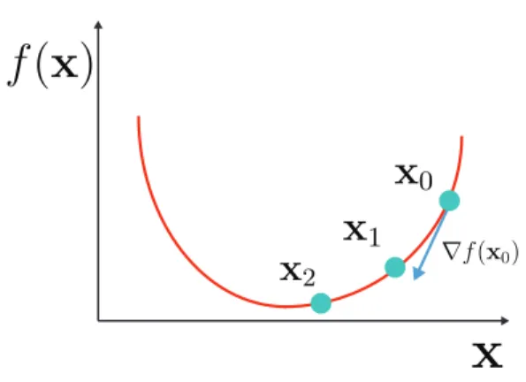
The idea of gradient descent dates back to Cauchy [33]. Figure 3-1 illustrates the process. For a loss function f (x), starting from an initial guess x0, we iteratively refine the guess using the

gradient ∇f (x):

xi+₁=xi− γ∇ f (xi), (3.4)

where γ is the step size parameter, sometimes called the learning rate, which determines how far we move along the negative gradient direction. Choosing the right step size is difficult, as it usually depends on the smoothness of the cost function, and typically the best step size is different for each dimension.

Figure 3-1: Gradient descent minimizes a function by iteratively following the negative gradient direction.

search methods. This means that they only find a local minimum of the function, while there can be a global minimum that is lower than the minimum they find.

Without any assumption on the function f , there is no guarantee that gradient descent will converge even to a local minimum. For example, if we reach a saddle point, the gradient would be zero and the iteration would stop. The convergence rate of gradient descent depends on how convex the function is (is it a “bowl shape” so that it only has a single minimum?), and whether it is Lipschitz continuous (is there a bound on how fast the function is changing?). Curious readers can consult textbooks (e.g. [26]) for more convergence proofs.

3.1.2 Stochastic Gradient Descent

In many applications, the gradient ∇f (x) we compute may not be fully accurate. For example, in regression, our cost function is a sum over example input-output pairs. If we have a huge database of example pairs, say one million, doing one step of gradient descent would require inefficiently enumerating all pairs of inputs and outputs. It would be desirable to randomly select a mini-batch each time we perform a gradient descent step (say, four from the one million). Furthermore, sometimes in an inverse problem, our forward model itself is a stochastic approximation to an integral (e.g. the rendering function in Chapter 5), and so is our loss function and gradients.

Fortunately, if our gradient approximation is unbiased (the expectation is the same as the true gradient) or consistent (the expectation converges to the true gradient if we use more samples), gradient descent can still converge to a local minimum [179, 36]. The condition for convergence is a gradually reducing step size γ over iterations, or equivalently, an increasing number of samples for gradient approximation. Intuitively, the noise we introduce in the gradient approximation brings some randomness to the steps in the gradient descent

iterations, but on average, they still go in the right direction. When we are closer to the optimum, the noise makes it harder to hit the exact optimum, so we either need to take smaller steps, or reduce the noise by increasing the number of samples.

In addition to computational efficiency, it is observed that the randomness can help stochastic gradient descent escapes from saddle points [55]. The noise also acts as an early stoppingmechanism [170, 76], which helps regression to generalize better to data not in the examples, thereby avoiding overfitting. See Chapter 3.3 for more discussions on this, and the relationship between stochastic gradient descent and other sampling-based methods.

3.1.3 Newton’s Method

Choosing the right step size for gradient descent methods is difficult and problem-dependent. Intuitively, for flat regions of cost functions, we want to choose a larger step size, while sharp regions require a smaller step size. Second-order derivatives are a good measure of how flat a function is: if the magnitude of the second-order derivatives is large, then the gradient is changing fast, so we should not take a large step.

In the 1D case, assuming the loss function always has positive second derivatives (which means it has a bowl shape or is convex), the update step of Newton’s method is

x_i+1= xi−

f′(x i)

f′′(x

i), (3.5)

where we replace the step size γ with the inverse of the second derivative.

To derive Newton’s method for the multivariate case, let us expand the loss function using the second-order Taylor expansion around xi:

f(xi+∆_x) ≈ f (xi) + ∇ f (xi)∆_x+ 1

2∆

T

xH(xi)∆_x, (3.6)

where H(xi)is the Hessian matrix. If we solve for the critical point of this approximation by

taking the gradient of ∆xand setting it to zero, we arrive at an update rule:

xi+₁=xi−H(xi)−1∇ f (xi). (3.7)

Essentially we replace the division of the second derivative in Equation 3.5 by multiplication by the inverse of the Hessian matrix.

Newton’s method can also be modified to work in a stochastic setting, where both the gradient and Hessian are an approximation to the true ones (e.g. [182, 183]).

disadvantages. First, the critical point of the Taylor expansion is not necessarily the minimum: it is only the minimum when the Hessian matrix is positive definite (all eigenvalues are posi-tive). Second, computing and inverting the Hessian is expensive in high-dimensional cases. Various methods address these issues. Quasi-Newton methods or Gauss-Newton methods approximate the Hessian using first-order derivatives. Hessian-free methods (e.g. [146]) use the Hessian-vector product (much cheaper than full Hessian computation) to obtain second-order information. Some methods approximate the Hessian using its diagonal (e.g. [147]). Adaptive gradient methods adjust the learning rate per dimension using the statistics of gradients from previous iterations.

Next, we will briefly introduce adaptive gradient methods, as we use them extensively in the following chapters. We will skip the discussions on Quasi-Newton, Gauss-Newton methods and others, since they are less relevant to this dissertation.

3.1.4 Adaptive Gradient Methods

How do we assess the flatness of a function, or how fast the gradients are changing, without looking at the second-order derivatives? The idea is to look at previous gradient descent iterations. The magnitude of the gradients is often a good indicator: if the magnitude is large, the function is changing fast. Adagrad [49] builds on this idea and uses the inverse of average gradient magnitude per dimension as the step size:

xi+₁=xi−

γ ⌈︂

G2_i + є○ ∇ f (xi), (3.8) where G2

i is a vector of the sum of the squared gradients at or before iteration i (the second

moment of the gradient), the division and the ○ here denote element-wise division and multiplication, and є is a small number (say, 10−8) to prevent division by zero.

Adagrad tends to reduce the learning rate quite aggressively, since it keeps the sum of squared gradient instead of average. Also, the smoothness of a function may be significantly different during the course of optimization. A possible modification is to only keep track of recent squared gradients. This can be done by an exponential moving average update (sometimes called an infinite impulse response filter):

G′

i2= αG′i−₁2+ (1 − α)∇f (xi)2, (3.9)