Climatology of the Great Plains low level jet using a balanced flow model with linear friction

Climatology of the Great Plains Low Level Jet Using a

Balanced Flow Model with Linear Friction

by

Stephanie Marder Vaughn

Submitted to the Department of Civil and Environmental

Engineering in Partial Fulfillment of the Requirements of the

Degree of Master of Science in Civil and Environmental Engineering

at the

Massachusetts Institute of Technology

June 1996

@ Massachusetts Institute of Technology 1996. All Rights Reserved.

Signature of Author... .. ... ... . . .... ...

Department of Civil and Environmenal Engineering March 29, 1996 Certified by... ... .... ... ... .. . Dara Entekhabi Associate Professor Thesis Supervisor •i . Chairman, Departmental iMASSACHUSETTS INS'ITiJ TE OF TECHNOLOGY

JUN

0

5 1996

Connmittee on Graduate Studih.

· 1

Climatology of the Great Plains Low Level Jet Using a

Balanced Flow Model with Linear Friction

by

Stephanie Marder Vaughn

Submitted to the Department of Civil and Environmental Engineering on March 29, 1996 in Partial Fulfillment of the Requirements of the Degree of Master of Science in Civil and Environmental Engineering

Abstract

The nighttime low-level-jet (LLJ) originating from the Gulf of Mexico carries moisture into the Great Plains area of the United States. The LLJ is considered to be a major contributor to the low-level transport of water vapor into this region. In order to study the effects of this jet on the climatology of the Great Plains, a balanced-flow model of low-level winds incorporating a linear friction assumption is applied.

Two summertime data sets are used in the analysis. The first covers an area from the Gulf of Mexico up to the Canadian border. This 10 x 10 resolution data is used, first, to determine the viability of the linear friction assumption and, second, to examine the extent of the LLJ _{effects. Wind speed is calculated as a function of temperature gradients,}

from which the linear friction parameter can be estimated. The predicted wind results are then compared to the actual wind measurements to determine the accuracy of the model. This analysis lead to a value of about 7 x 10-5 s- for the linear friction parameter, and predicted results within one standard deviation of the actual data. Maximum LLJ effects were found to occur around the Northern Texas-Oklahoma border.

The second data set is taken from Blackwell, Oklahoma. This data includes measurements of relative humidity and precipitation, as well as wind and temperature data, and was used to determine the humidity flux through this region, its consequences, and the effect of the LLJ _{on this flux. The data is recorded every fifteen minutes for June, July,}

and August of 1994, so it was useful in examining the diurnal cycle of the wind components and the humidity flux. The effects of the LLJ were found to reach this northern Oklahoma location and to have an effect on the low-level vapor transport through the region.

Thesis Supervisor: Dara Entekhabi

Acknowledgments

This research has been partially supported by National Aeronautics and Space Administration research grant NAGW-4164 and National Science Foundation Fellowship 9354923-GER. Professor Ken Crawford, state climatologist for Oklahoma, provided the data used in Chapter 4.

Contents

CHAPTER 1 - INTRODUCTION ... 13

1.1 LAND-ATMOSPHERE INTERACTION... ... ... 13

1.2 REVIEW OF CONTINENTALITY ... 14

1.3 REVIEW OF PREVIOUS MODEL ... ... 16

1.4 REVIEW OF THE LOW LEVEL JET ... 16

CHAPTER 2 - WINDS MODEL ... 20

2.1 MOMENTUM EQUATION ... ... 20

2.2 LINEAR FRICTION ... ... .. ... 23

2.3 PRESSURE-TEMPERATURE RELATIONSHIP ... ... 24

2.4 LOW-LEVEL WIND EQUATIONS ... ... ... .. 28

CHAPTER 3 - ISLSCP DATA ANALYSIS... ... 30

3.1 DESCRIPTION OF DATA AND ANALYSIS METHOD ... 30

3.2 RESULTS OF PARAMETER ESTIMATION ... 32

3.3 SPECIAL CASE: DT / DX EQUALS ZERO ... 37

3.4 ERR()R ESTIM ATION ... ... ... 40

3.5 EXAMPLE: AUGUST DATA AT 0006 GMT ... 44

3.6 ISLSCP ANALYSIS FOR CONTINENTALITY... 48

CHAPTER 4 - OKLAHOMA DATA ANALYSIS ... 53

4.1 DESCRIPTION OF DATA AND ANALYSIS METHOD ... 53

4.2 CASE: AUiUST 15T_{H, 1994 ... ... 55}

4.3 OKLAHOMA DATA ANALYSIS ... ... 61

CHAPTER 5 - CONCLUSIONS AND FUTURE RESEARCH ... 67

5.1 CONCLUSIONS ... ... ... ... 67

5.2 FUTURE RESEARCH ... .. .... ... .... . ... 68

APPENDIX A - ALTERNATE DERIVATION OF TEMPERATURE-PRESSURE RELATIONSHIP ... ... 69

List of Figures

FIGURE 1.1 - CONCEPTUAL DIAGRAM OF THE PATHWAYS THROUGH WHICH SOIL

TEMPERATURE, SOIL MOISTURE, NEAR-SURFACE AIR HUMIDITY, AND NEAR-SURFACE AIR TEMPERATURE MUTUALLY INFLUENCE ONE ANOTHER (FROM BRUBAKER, 1994). 13 FIGURE 1.2 - DECREASE IN THE MEAN DAILY JULY TEMPERATURE AND INCREASE IN

DIURNAL RANGE OF TEMPERATURE WITH DISTANCE INLAND (FROM ENTEKHABI ET AL.,

19 9 4 ) ... 1 5

FIGURE 1.3 - TOTAL (A) AND NIGHT (1800-0600 CST) MINUS DAY (0600-1800CST) (B)

TIME-MEAN MOISTURE FLUX AND BUDGET FOR A TWO-MONTH (MAY-JUNE) MODEL

SIMULATION. SIZE OF REGION IS 7.54 X 106 KM. (FROM HELFAND ET AL., 1995)... 19

FIGURE 2.1 - DIAGRAM SHOWING BALANCE OF PRESSURE, CORIOLIS, AND FRICTIONAL FORCES WITH WIND FOR UNIFORM FLOW IN THE NORTHERN HEMISPHERE. SOLID LINES REPRESENT ISOBARS IN A HORIZONTAL PLANE (FROM WALLACE ET. AL., 1977)... 23

FIGURE 3.1 - MAP OF REGION. RECTANGLE SHOWS AREA STUDIED IN THIS ANALYSIS... 31

FIGURE 3.2 - RESULTS OF PARAMETER ESTIMATION FOR JJA DATA ANALYSIS ... 35

FIGURE 3.3 - RESULTS OF MONTHLY AVERAGE PARAMETER ESTIMATION... 36

FIGURE 3.4 - RESULTS OF PARAMETER ESTIMATION FOR JJA TAKING DT/DX = 0... 38

FIGURE 3.5 - RESULTS OF MONTHLY AVERAGE PARAMETER ESTIMATION, TAKING DT/DX = 0... ... .. ... ... ... 39

FIGURE 3.6 - ERROR RESULTS OF U AND V FOR JJA WHERE BAR INDICATES RMS ERROR, SQUARE SHOWS AVERAGE VALUE, AND ERROR LINES INDICATE ONE STANDARD D EV IA TION . ... 42

FIGURE 3.7 - SAME AS FIGURE 3.6 FOR MONTHLY AVERAGE RESULTS... 43

FIGURE 3.8 - FOR AUGUST, 0006 GMT, A -ACTUAL AND DERIVED TEMPERATURE FIELD; B -DERIVED TEMPERATURE LAPSE RATE FIELDS; C - ACTUAL AND DERIVED ZONAL WIND FIELD. ... ... 46

FIGURE 3.9 - FOR AUGUST, 0006 GMT, A - ACTUAL MERIDIONAL VELOCITY FIELD; B -DERIVED MERIDIONAL VELOCITY FIELD; C - DERIVED FIELD, DT/DX = 0. ... 47

FIGURE 3.10- ACTUAL AND DIURNAL RANGE OF TEMPERATURE ALONG TRANSECT AT 97.50 LONGITUDE FOR JUNE, JULY, AND AUGUST ... ... ... 49

FIGURE 3.11 - AVERAGE DAILY (A) ACTUAL AND DIURNAL RANGE OF TEMPERATURE, (B) ACTUAL U AND V WIND COMPONENTS AND (C) TEMPERATURE LAPSE RATE AT 97.50 W

FOR AUGUST. ... .... ... ... 50

FIGURE 3.12 - ABSOLUTE VALUE OF AUGUST WIND ANOMALIES (MEAN DAILY -HOURLY

VALUE) AT 97.50 _{W ...}

... 52

FIGURE 4.1 - DIAGRAM SHOWING HOW TO CALCULATE U AND V WIND COMPONENTS ... 54

FIGURE 4.2 -TOTAL (A) U AND (B) V WIND COMPONENTS ON AUGUST 15TH, 1994 AT

BLACKWELL, OK ... 57

FIGURE 4.3 - AUGUST 15T' A -WIND SPEED; B - WIND DIRECTION; C - VAPOR DENSITY; AND

D -AIR TEMPERATURE AT BLACKWELL, OK. ... 58

FIGURE 4.4 - AUGUST 15 TH, 1994 TOTAL HUMIDITY FLUX ... ... 59

FIGURE 4.5 - FOR AUGUST 15TH , A -PRESSURE; B -RELATIVE HUMIDITY; AND C -SOLAR

RADIATION... ... 60

FIGURE 4.6 - JJA 1994 AVERAGE VALUES FOR U AND V, TOTAL (A AND B) AND FILTERED (C

AND D), AT BLACKWELL, OKLAHOMA. BARS ON TOTAL DATA INDICATE ONE

STANDARD DEVIATION ... ... ... .... ... 63

FIGURE 4.7 - SAME AS FIGURE 5.5, SHOWING HUMIDITY FLUX ... 64

FIGURE 4.8 - AVERAGE JJA DAILY (A) SOLAR RADIATION, (B) PRESSURE, (C ) RAIN, AND

(D) RELATIVE HUMIDITY AT BLACKWELL, OK ... 65

FIGURE 4.9 - AVERAGE JJA DAILY (A) WIND SPEED, (B) WIND DIRECTION, (C ) VAPOR

List of Tables

TABLE 3.1 - RESULTS OF K ESTIMATION (S X 10 ) _{... ...}

... 33

TABLE 3.2 - RESULTS OF ESTIMATION OF PARAMETER 'A' (M2 _S-1 _{K X 10}4) _{... 33}

TABLE 3.3 -RESULTS OF ESTIMATION OF PARAMETER 'B' ( )... 33

TABLE 3.4 - _{AVERAGE RESULTS OF JJA OVER EACH TIME PERIOD ... ... 34}

TABLE 3.5 - RESULTS OF ESTIMATION OF PARAMETER K (S-' X 10"5), DT/DX = 0... 37

TABLE 3.6 - RESULTS OF ESTIMATION OF PARAMETER A (M2 _{S- K- x 104), DT/DX = 0. ... 40}

TABLE 3.7 -RESULTS OF ESTIMATION OF PARAMETER B ( ), DT/DX = 0. ... 40

TABLE 3.8 - AVERAGE RESULTS OF JJA OVER EACH TIME PERIOD, DT/DX = 0... 40

TABLE 3.9 - JUNE RMS (MEAN) SUMMARY ... ... 41

TABLE 3.10 - JULY RMS (MEAN) SUMMARY ... 41

TABLE 3.11 - AUGUST RMS (MEAN) SUMMARY ... ... 41

TABLE 3.12 - MONTHLY AVERAGE RMS (MEAN) SUMMARY ... 44

Chapter 1 - Introduction

1.1 Land-Atmosphere Interaction

In order to accurately represent atmospheric phenomena, knowledge of the processes occurring from the atmosphere, from the land, and how they interact is necessary. The atmosphere affects the land and oceans through such factors as solar radiation and clouds. The land, in turn, affects the atmosphere through evapotranspiration and radiative heating, for example. These processes form a two-way coupled system where one component can not be ignored without losing significant information.

u'"4 1PYlO'ivi vaOa'usl1W

11

soil thermal

_radiation

soil sensible

heat flux

latent heat

flux

diness

vection

intal

rgy

absorption

RECIPITATION

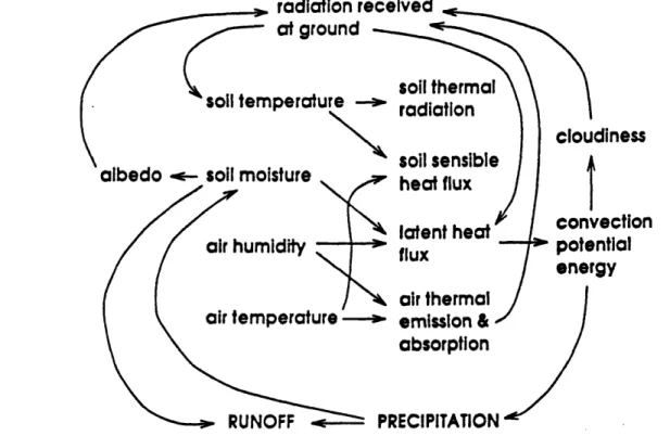
Figure 1.1 -Conceptual diagram of the pathways through which soil temperature, soil moisture, near-surface air humidity, and near-surface air temperature mutually influence one another (from Brubaker, 1994).

The land and atmosphere are linked by exchanges of energy, mass, and momentum. This exchange is controlled in large part by the moisture and heat states of the land. Figure 1.1 is a conceptual diagram showing how these factors affect each other.

This is just one example of the many feedback mechanisms that exist, which can ultimately lead to anomalous conditions such as droughts. The problem is complicated by the fact that the solar forcing leads to a wide range of variability covering time scales from decades to seconds. Further, water adds additional complexity due to the fact that it exists

in all three phases -liquid, solid, and gas -in the atmosphere; large amounts of heat uptake

and release are associated with the phase changes.

The study of land atmosphere-interaction specifically is relatively new. But it has long been recognized that surface processes are important in understanding the overall climate (Entekhabi, 1995).

1.2 Review of Continentality

Climate variability over continental land regions exhibit unique characteristics that arise in large part from the land-atmosphere interaction processes described in the previous section. Continentality refers to the effect that a large land area has on the climate. It does not cover orographic effects. For example, consider soil moisture. A simplified description of the states of water in the hydrologic cycle is as follows (from Entekhabi et al., 1994). Precipitation occurs, and leads immediately to storm runoff After a delay, soil moisture increases, which then adds to streamflow, and finally the rain event reaches the groundwater. The net effect of the lag times between the actual rain occurrence and the appearance of this moisture in the different media leads to a dampening of the fluctuations caused by the rain, and thus prolonged hydrologic anomalies (i.e. drought or flood). Now consider that as soil moisture increases, so does evapotranspiration, and eventually rainfall. This causes a positive feedback loop that decreases the drought effects. This process may be termed precipitation recycling, and is

an example of continentality. McNab et al. (1983) found that inter-continental regions are more prone to persistent anomalies such as droughts or floods.

As one moves inland, moisture effects from the ocean are diminished. It is not surprising that precipitation decreases with distance inland, as does the relative humidity.

28

32

36

40

44

₄₈

Latitude

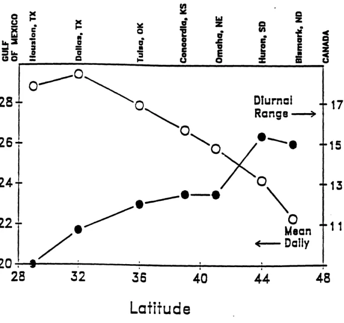
Figure 1.2 -Decrease in the mean daily July temperature and increase in diurnal range of temperature with distance inland (from Entekhabi et al., 1994).

28

26

24

22

20

17

15

13

11

In order to find evidence of continentality, Entekhabi et al. (1994) suggests looking at three criteria, all with respect to distance inland. These are an increased diurnal range of temperature, decreased humidity, and the dominant precipitation and wind patterns (see Figure 1.2). As part of this analysis, the data used will be examined for such continental effects.

1.3 Review of Previous Model

Brubaker (1995) developed a 1-D in the vertical, 4-state land-atmosphere interaction model. The model looks at the time-evolution of four coupled variables. The energy states are ground and air potential temperature and the water states are soil moisture and humidity. The two forcings are solar radiation and wind speed. The model incorporates the land-atmosphere interaction processes through a set of four coupled differential equations, one for each of the state variables. It looks at the temporal, but not

spatial, variation of factors.

Once including stochastic variation, the model does a good job of displaying persistence of anomalous conditions. The next step is to incorporate variable wind speeds and extend the model to 2-D along a transect of longitude, thus allowing the study of continentality. The area chosen to initially perform this analysis on is the Great Plains area of the United States, and thus this thesis will help determine how wind should be parameterized.

1.4 Review of the Low Level Jet

It has been observed that a nocturnal low level jet (LLJ) occurs over the Great Plains of the United States, originating from the Gulf of Mexico. Numerous studies have examined this phenomenon (for example, Bonner et al., 1970; Helfand, 1995). There are

many theories as to the cause of this jet. Two predominant ones are that it is due to inertial oscillations or baroclinicity over sloping terrain.

During the day, there is much turbulence in the mixed layer and friction retards wind speed greatly. This leads to sub-geostrophic winds, where the geostrophic wind is a standard assumption which neglects frictional effects, and assumes that the pressure force is balanced by the coriolis force. At night, however, the geostrophic approximation is more reasonable since turbulence is reduced. The coriolis force then plays a stronger role in affecting wind speed, deflects the wind to the right (in the northern hemisphere) and may actually lead to super-geostrophic winds (Stull, 1988). This phenomenon is termed inertial oscillation. The wind varies between sub- and super- geostrophic between day and night. This super-geostrophic wind is the LLJ. Stull (1988) suggests an inertial period of 27t/f,, where f, is the coriolis force. This implies a period of about 17 hours in mid-latitudes. However, Dutton (1976) states that pure inertial oscillations do not really exist,

due to friction, time lags, and other forces.

An alternate explanation is that of the thermal wind. During the day, LLJ occurrence is reduced due to turbulence. Over sloping terrain at night, the wind may be strongly driven by temperature gradients, since wind flows from areas of high to low

pressure.

Regardless of the causes, the patterns and effects of the LLJ are observed. Helfand (1995) found that the LLJ starts as a south-easterly flow from the Gulf of Mexico. The flow becomes southerly over the Great Plains, and then turns south-westerly over the Eastern US. It thus has an anti-cyclonic (clockwise in the Northern Hemisphere) rotation. The jet occurs most frequently from April to September, and is strongest at night. The diurnal cycle of the LLJ is greatly reduced as altitude increases, and this may be due mostly to lessening friction. Bonner (1970) found day to night wind speed variations from 5 to 9 m/s, and a maximum wind speed between 00 and 03 Central Standard Time (CST), where CST equals GMT minus 6 hours. The amplitude of the oscillation was found to be about 2 to 3 m/s, and maximum winds have been found to occur in Central Texas and Oklahoma.

One of the major effects of the LLJ is the northward transport of moisture that it causes. The primary source of water vapor in the Great Plains originates from 150_{N to}

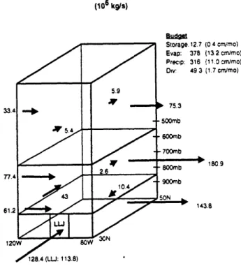
35'N (Rasmusson, 1967). As a reference point, the border of Texas with the Gulf is at about 300_{N, 97}0_{W. Helfand (1995) found that the moisture flux increases by 40% at}

night. He states two reasons that the LLJ is an important factor in moisture transport. First, the jet contributes to the overall mean-flow pattern. It is not the diurnal fluctuations that really have an effect, but rather their effect on the mean-wind. Second, the diurnal cycle and the disruptions it causes in the mean flow do contribute to the effect of the transient transport. The total moisture influx at 1000_{W, 30}0_{N was found to be 128.4x10}6

kg/s, and 113.8x106 _{kg/s was found to occur from the LLJ forcing alone (Helfand, 1995,}

see Figure 1.3). This implies that the jet is supplying one-third of the moisture to the Plains. This estimate is consistent with the study by Brubaker et al. (1994) in which vapor convergence over the Midwest is shown to be strongly affected by low-level flow from the Gulf of Mexico. The maximum northward transport occurs at around 400_{N, but effects are}

still felt across the Canadian border (Rasmusson, 1967).

This study will attempt to find evidence of these effects. The ISLSCP data will be useful in determining the extent and magnitude of the LLJ over the entire Great Plains. The Oklahoma data includes moisture variables which will allow examination of day to night changes in moisture transport. The following chapter describes the model equations used in this analysis.

Budget (0 4 cmirno) (13.2 cmimo) (11.0 cm/mo) (1.7 cm/mo) 180.9 Budaet tNiwoDfM"2 .171 6 ;-6 crr.fo) 3147 1-11 cr;im• 137 7 i-4 5:.Pr1mo 55 4 (-0 2 •,m/mo)

Figure 1.3 - Total (a) and night (1800-0600 CST) minus day (0600-1800CST) (b) time-mean moisture flux and budget for a two-month (May-June) model simulation. Size of region is 7.54 x 106 km. (from Helfand et al., 1995).

May/June Moisture Flux Over Continental U.S.

(106 kg/s)

Night-Day May/June Moisture Flux Over Continental U.S.

(106 kg/s)

Chapter 2

-

Winds Model

Wind is an important component of boundary layer analysis. It is forced by gradients in surface heating and by the coriolis force, and is needed for transport of heat and moisture. In this model, wind is determined as a function of temperature, coriolis force, and friction. This chapter describes the derivation of these wind equations.

2.1 Momentum Equation

The basis for the wind model used in this study is the 2-D steady-state momentum equation. Given that u is the east-west component of the wind, and v is the north-south component, the equation of motion states that:

D _(Forces)

Dt

(2.1)

where

D =" o "

Dt or "xn c d

is the "material" or "substantial" derivative (in 2-D).

Consider an elemental volume of air, 6x6y5z. The mass of this volume is then

p6x6y6z. If a force acting on this volume is divided by the mass of the element, then an

acceleration (units LT-2) results. The following four sections describe the forces acting on a volume element of air, in terms of acceleration.

Pressure Force

F,

P = VP (2.2)

mn

_p

This is simply the net pressure acting on the elemental volume.

Coriolis Force

The coriolis force is an apparent force that acts on an object moving with respect to a rotating field, and is required in order for Newton's Second Law to hold. It acts to deflect an object to the right of the direction of motion. A full derivation is not included here, but the resulting expression is

f = 2O sin 0 (2.3)

where Q = the angular velocity of the earth (7.292x10-5 _{s-') and}

₄

_{is the latitude.}

Frictional Force

It is on this term that a majority of the work in this study pivots. A linear friction parameterization can be made of the form

SFx = -ku

m _(2.4)

1 F,, = -

m-k, the linear friction parameter, is the parameter (units time') this study attempts to estimate. Its value is generally taken to be around 3x10-5 s-1, but it depends on factors such as surface roughness, wind speed, and static stability. Section 2.2 will cover the validity of this assumption in more depth.

Other Forces

There are two other relevant forces - gravitational and centrifugal. Gravitational force is dependent on the mass of two objects being attracted and the disatnce between these objects. Centrifugal forces act in towards the axis of rotation and depend on the angular momentum of the object and it's distance from the center of rotation. Like the coriolis force, it is apparent, and is usually incorporated into the gravitational force.

Both of the above are ignored in this study, however, since they act in the vertical z-direction.

Now that all of the forces are defined, we can return to Equation (2.1), and incorporate Equations (2.2) through (2.4) into it. Assuming steady-state, d/dt -+ 0

f -. - ku = 0 (2.5a)

P &3(

This is the basic form of the linear-friction and balanced-flow momentum equation used in this study. The last adjustment to make is that of defining the pressure in terms of surface temperature.

2.2 Linear Friction

Friction acts to retard the motion of air, and increases as the height above ground-level decreases. It therefore acts in a direction opposite to the velocity vector v, making wind in the lowest kilometer or so of the atmosphere sub-geostrophic. As was touched on in the previous section, geostrophic flow assumes that the coriolis force perfectly balances the pressure force. This is a valid assumption in many cases, but not in this study, where we are looking at winds measured at about 10 meters above ground.

L

p-28p

p-2Sp

V

H

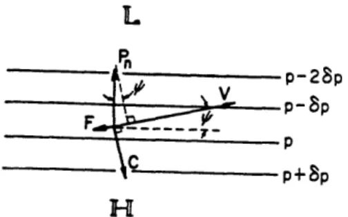
Figure 2.1 -Diagram showing balance of pressure, coriolis, and frictional forces with wind for uniform flow in the northern hemisphere. Solid lines represent isobars in a horizontal plane (from Wallace et. al., 1977).

Figure 2.1 ( from Wallace et al, 1977) illustrates the balance between pressure, coriolis force, and friction required in the Northern Hemisphere. The dashed line represents the geostrophic wind, and therefore the larger the linear friction constant 'k' is, the larger is the angle between the geostrophic and subgeostrophic wind. Since we are assuming that the frictional force is a linear function of u and v, k can be thought of as a linear damping coefficient. This parameter was estimated as part of this study, and the results are shown in Chapter 3.

In order to determine whether including friction is necessary, Dutton (1976)

suggests looking at two parameters - the Rossby number and the Reynolds number. The

Rossby number measures the ratio of inertial terms to the coriolis force and the Reynolds number is the ratio of inertial to viscous terms. They are equal to:

Ro

=--gL

Re =

where f is the coriolis parameter, v is the wind vector, L is the relevant length scale, and v is the viscosity. If the Rossby number is small, the Reynolds number is large, and the flow is slowly varying, then the geostrophic approximation is probably sufficient. The magnitude of these variables will be looked at in this analysis.

2.3 Pressure-Temperature Relationship

From the surface energy balance we obtain an estimate of surface temperature. We would like to find a relationship to convert the pressure term of the momentum equation to a

temperature term. Two derivations of the relationship used were performed. The first is shown below, and the second is included as an appendix.

The Poisson Equation states that (Wallace et al, 1977):

T =

o0

_-) C

\Po) (2.7)

Where 0 is the potential temperature, Rd is the dry air gas constant (287 J deg-' kg'), C, is the specific heat (1004 J deg' kg-'), and Po is the standard pressure (taken as 1000 mb).

Differentiating along lines of constant 0 (isentropic surfaces) with respect to x results in:

dx

OK(idP) 0 W p K-] R P PCP (d

Rd

T (dP

K-I P 0o (2.8)

In the above, K is equal to Rd / Cp. Using three rules - the chain rule, the hydrostatic

relationship, and the ideal gas law -it can be shown that

p

dx)

dx

d- (CT +gZ)

First, applying the chain rule to expand dP/dx from Equation (2.8) leads to

dP

ýdxP)

dP dzdz - - dxJV- I

(2.10)

The hydrostatic relation

dP

dz

can then be substituted into Equation (2.10), which results in

(2.12)

+ Pg d

Now, substitute for (dP/dx)o using Equation (2.8)

(2.11) (2.9)

PC dT

RdT dx

0

CdP

dx

(+

dz

dx

19 (2.13) odP

dx ,

M~ \M-~/

dP

ýdxP)

dPo

_{dx ,}

Finally, use the ideal gas law in order to eliminate pressure from the right hand side of Equation (2.13):

P = pRd

T

(2.14)

Note that the (P/RT) multiplying the dT/dx term of Equation (2.13) is equal to p. Therefore, i dPJ = Cp _{+g( dg )} oV or, rearranging: p dP

p

dx

=

dx

(CpT+ gz) (2.15)

The term - (gz)o is the effect of topography on the pressure gradient force.' In the dx

absence of orography,

dP

= C p dT (2.16a)

P I d

dT

= Cd

"

dz

(2.16b)

2.4 Low-Level Wind Equations

To arrive at the final form of the wind equations used in this model, combine Equations (2.5a) and (2.5b)

fi,

ku = 0

-.

fi

-

k

=

0

with Equations (2.16a) and (2.16b), respectively,

I dP

p

dxP)

1 dP

p dy) dT Pdx CdT = Cp y, to obtain

ft - C - ku = 0 (2.17a)

Jr/"

- fi -C

-

lkv = 0

(2.17b)

Solving Equations (2.17a) and (2.17b) simultaneously for the u and v wind components leads to the final form of the wind equation used in this model:

u = -a + b (2.18) v &a -b where

f

a= - CP

k' +f

-k

b-(2.19)

Note that the constants a and b multiplying the temperature gradients are equal and opposite for the u and v equations. Recall k is the linear friction constant and f is the coriolis force.

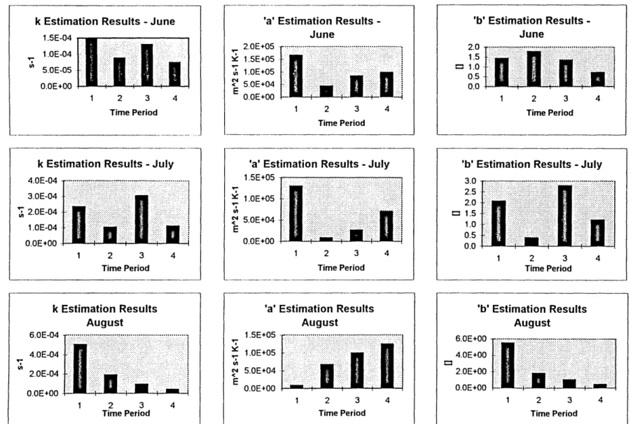
'a' Estimation Results -June ~ ~:~::~: , .•::~<:••:::~.«•.:::::::::::...:..:••":":••}...••••••••

"'J

~ ~~~:~I;1U

'b' Estimation Results -June c

1:1

t:·i:):·:f·lj;I~:1i·i~j:!j·:I;l:l

Time Period

k Estimation Results - June

15E_ M

IIiDI

1 OE 04 ..•..•...•..•. ••.•...•••..•.•..••..•..•.•..••...••:..•.:.. :.. :..:::.:•.•....••...•.:.•..•.: ....•.:.•..:.:::•.•••••..••..•:•.:..••:•..:: •...•:...::.••:.:.:•.:•••.. - •-. ..:, :- .: '..:. .', ,'":." . . ~.

:::

»>

::::» ':>:\>"-"',"':: III 5.0E-05' ...:::: >/:.

<:

. . ,-."-:..:,:. ...:::::::.- ><: O.OE +00 " '. ' : . : . : . ' 1 2 3 4 Time Period 2 3 4 2 3 4 Time Period 4 2 3 Time Period

'b' Estimation Results - July

3.0 r·:·~<::·<:·<7.:::·::<:<::<:<::·::«<::·:::··::<:·::<:::·:·:<:=7.1 2.5· 2.0 :::::: 1.5 1.0 .

~:~~

4 2 3 Time Period

'a' Estimation Results - July

1.5E+05"r',-,....,..,.,..,....-.,...,.,.,...,...,.,....-.,...,.,.,...~....,..-"

...

~ 1.0E+05

...

en ~ 5.0E+04 . E O.OE+OO ' 3 2 Time k Estimation Results 4.OE-04 -r.~: ««::~~~.<:~~.<..~< < . 3.0E-04 J; 2.0E-04 1.0E-04 ' O.OE+OO w Vl 'b' Estimation Results August c

~:~~~~rllll;~1

1 2 3 4 Time Period 4 3 2 Time Period O.OE+OO I - I - I

'a' Estimation Results August 1.5E+05 .r:::,""",:.:~.,

..

::".:,::::::,',::,:.:.,:,:,~,,:,':.'::.:'::':':'::

...

~ 1.0E+05 III , ... N 5.0E+04 < E 4.0E-04 6.0E-04 2 3 4 Time Period k Estimation Results August O.OE+OO

...

en • 2.0E-04·

The overall average value of k obtained is 7.51 x 10-05 s-_{'. The existing literature (Wallace, 1977;}

Dutton, 1976) on linear friction states that k should be approximately 2.7 x 10"05 s~'. The results derived in this study are relatively close to this value, and may be more appropriate for the

specific region evaluated here.

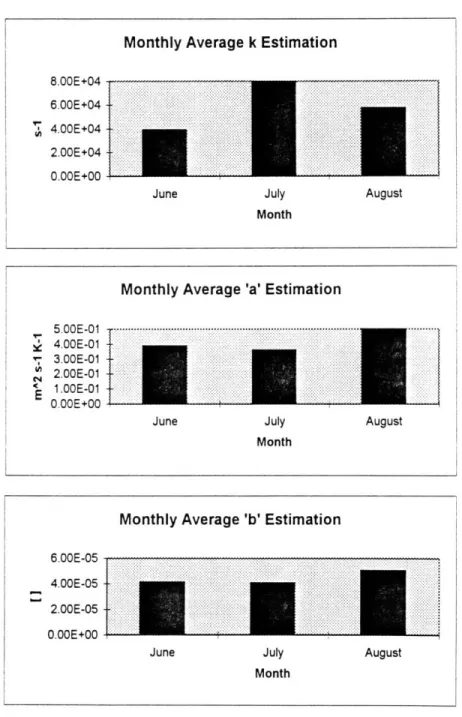
Monthly Average k Estimation 8.00E+04

6.OOE+04 S4.00E+04 2.00E+04

0.00E+00

I June July August

Month

Monthly Average 'a' Estimation

5.00E-01 ' 4.00E-01 3.00E-01 0 2.00E-01 1.00E-01 000E+00

June July August

Month

Monthly Average 'b' Estimation

June July August

Month

Figure 3.3 - Results of monthly average parameter estimation.

6.00E-05

4.00E-05

2.00E-05 O.OOE+00

Chapter 3

-

ISLSCP Data Analysis

In order to examine, first, the value of the linear friction parameter, and, second, evidence of the low-level-jet, an analysis was performed on a large data set covering the Great Plains from the Gulf of Mexico up to the Canadian Border. Chapter 4 goes on to describe a second data analysis performed at a specific site in Oklahoma, used to look at a more detailed diurnal cycle of conditions in this area, and the subsequent transport of water vapor.

3.1 Description of Data and Analysis Method

The data used in this analysis came from ISLSCP -the International Satellite Land Surface Climatology Project, a division of the World Climate Research Program - Global Energy Water Cycle Experiment (WCRP-GEWEX). Data is recorded on a global 10 x 1o grid. The variables collected fall into five categories - vegetation, hydrology and soils, snow, ice, and oceans, radiation and clouds, and near-surface meteorology. This study looks at the near-surface meteorology group, specifically the u and v components of the wind vector at 10 m. and the temperature at 2m. Monthly 6-hourly data for June, July, and August of 1987 was used. This means that the data was averaged over the four 6-hour periods of the day for the entire month (i.e. 0000, 0006, 0012, and 0018 GMT).

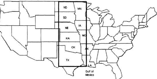
The area chosen to study extends from 30.5 to 55.5 latitude, and 92.5 to 102.5 longitude. This covers the Great Plains area of the United States, and extends northward to the Canadian border (see Figure 3.1). First, a 2-D fourth-order polynomial was fit to the actual temperature field. The x- and y- partial derivatives of this polynomial were then used to calculate the GcT/cx and PT/cy fields. The length scales used in taking these

Figure 3.1 -Map of region. Rectangle shows area studied in this analysis.

derivatives were determined according to Morel (1973) as:

1 Latitude(O) = R = 1.1 lxl06 (3.1)

1' Longitude(Z) = R cos(0)

where R is the mean radius of the earth and 0 is in radians. Then the actual u and v wind fields were fit to the temperature derivatives in such a way that the parameters a and b, as described in Section 2.4, were forced to be equal for u and v. To illustrate, recall that

u = -a + b

(3.2)

If all terms in these equations are thought of as vectors, then the two equations can be solved simultaneously for a and b. The resulting expressions are:

-V +11

(3.3)

07 c7

b= k

--

V +

.f

The average values of a and b for each time period of each month were determined, and finally the linear friction parameter could be estimated according k = bf, where f is the coriolis parameter.

Once the parameters were determined, a and b were used to calculate fit velocity fields according to Equation (3.2) above. The correlation between the fit and actual velocity was used to determine how well this linear friction parameterization works.

3.2 Results of Parameter Estimation

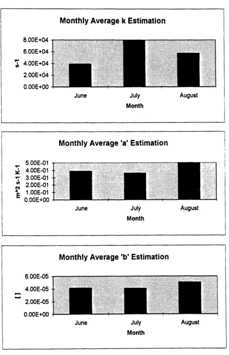
The results of the parameter estimation as described in the previous section are shown in Tables 3.1 through 3.4, and presented graphically as Figures 3.2 and 3.3. The monthly average results were determined by first averaging the actual data, and then

performing the same analysis on the averaged data that was performed on each individual time period's data.

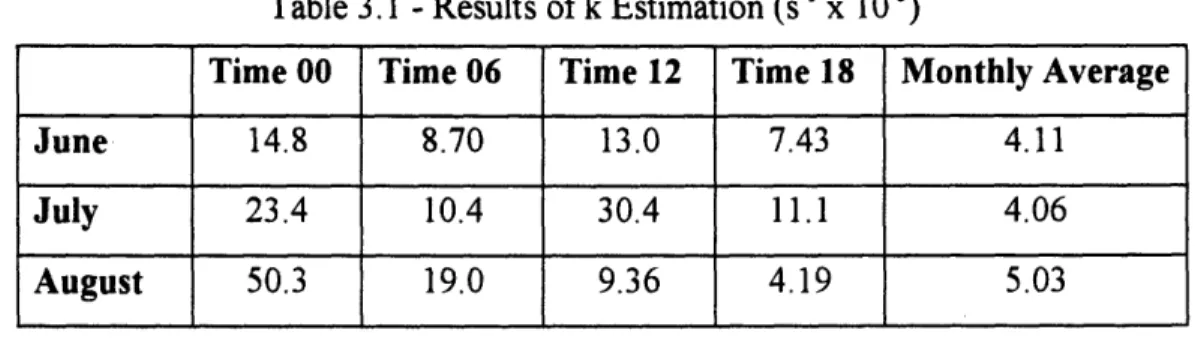
Table 3.1 -Results of k Estimation (s1' x 10-5 )

Time 00 Time 06 Time 12 Time 18 Monthly Average

June 14.8 8.70 13.0 7.43 4.11

July 23.4 10.4 30.4 11.1 4.06

August 50.3 19.0 9.36 4.19 5.03

Table 3.2 -Results of Estimation of Parameter 'a' (m2 _{s-' K-' x 104)}

Time 00 Time 06 Time 12 Time 18 Monthly Average

June 16.60 4.30 8.40 9.72 3.88

July 13.00 0.83 2.64 7.01 7.98

August 0.87 6.66 9.98 12.5 5.73

Table 3.3 -Results of Estimation of Parameter 'b' ()

Time 00 Time 06 Time 12 Time 18 Monthly Average

June 1.43 1.77 1.35 0.72 0.39

July 2.07 0.38 2.79 1.21 0.36

August 5.49 1.79 1.03 0.45 0.50

If the above values are averaged over each month for a particular time period, the results

Table 3.4 - Average results of JJA over each time period

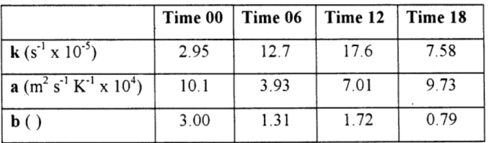
Time 00 Time 06 Time 12 Time 18 k (s-' x 105) 2.95 12.7 17.6 7.58

a (m2 s-' K-' x 104) 10.1 3.93 7.01 9.73

The overall average value of k obtained is 7.51 x 10-s _s"1. _{The existing literature (Wallace, 1977;}

Dutton, 1976) on linear friction states that k should be approximately 2.7 x 10.05 s"_{'. The results}

derived in this study are relatively close to this value, and may be more appropriate for the specific region evaluated here.

Monthly Average 'a' Estimation 5.00E-01 Y 4.00E-01 3.00E-01 S2.00E-011.00E-01 1.OOE-00 O.OOE+00

June July August

Month

Monthly Average 'b' Estimation

Figure 3.3 -Results of monthly average parameter estimation.

6.OOE-05

4.00E-05 2.00E-05

0.OOE+00

June July August

Month

... . . ..

.. .... .. ..:-·

3.3 Special Case: dT / dx equals zero

The change in temperature in the y-direction (with latitude) is probably more important in determining the v component of the wind than is the change in temperature with longitude. Using this assumption, an analysis of the data was performed setting dT/dx = 0 and using the average u over the region, u,vg. Making the necessary substitutions into the equations described in Section 3.1, the new relevant system becomes:

S= -a

--v =

-ab-(3.4)

a=u

lal'

Tables 3.5 through 3.10 and Figure 3.4 show the results of this analysis. The overall average value of k obtained through this analysis is 7.97 x 10-04, a value that is an order of magnitude less than that obtained in the full analysis.

Table 3.5 -Results of Estimation of Parameter k (s~_{' x 10-5), dT/dx = 0}

Time 00 Time 06 Time 12 Time 18 Monthly Average

June 14.3 382.0 14.4 28.7 79.5

July 36.1 20.9 212.0 33.0 21.8

Monthly Average k Estimation - dT/dx = 0 2.00E+05 1.50E+05 1.00E+05 5.00E+04 0.00E+00

June July August

Month

Monthly Average 'a' Estimation -dT/dx = 0

2.00E+01 . 1.50E+01

' 1.00E+01

5.00E+00

0.00E+00

June July August

Month

Monthly Average 'b' Estimation - dT/dx = 0

June July August

Month

Figure 3.5 -Results of monthly average parameter estimation, taking dT/dx = 0.

1.50E-03 1.00E-03 5.00E-04 0.00E+00 ____ __ i

i

...~ ~U~S i .·.·.·..·...·.·.·.?_:: :·:·:·:·:·:·:·:·:·~ ::::::::::::::::::s ~i

Table 3.6 -Results of Estimation of Parameter a (mi2_{s-1 K x 104), dT/dx =}

0.

Table 3.7 -Results of Estimation of Parameter b (), dT/dx = 0.

Time 00 Time 06 Time 12 Time 18 Monthly Average

June 1.70 43.5 1.62 3.42 9.18

July 4.45 2.45 24.8 3.97 2.60

August 0.99 4.77 1.32 2.35 18.0

Table 3.8 -Average results of JJA over each time period, dT/dx = 0.

3.4 Error Estimation

Now the question becomes how well does this parameterization work. Tables 3.9 through 3.12 tabulate the root mean square (RMS) error between the actual and derived results. RMS is calculated as

Time 00 Time 06 Time 12 Time 18

k (s1 x 10-5) 18.8 147.0 78.9 26.3

a (m2 _{S-1 K-' x 104) 16.2 1.60 9.49 57.4}

RA4'S

= VJ-JZ- O yi.actual -yi.ppected

(3.5)

It is clear that August is the month most amenable to this linear friction assumption. Times are given in GMT, so that the period from 0006 to 0012 GMT is midnight to 6:00 am locally. The value of the mean winds are included for comparison in parentheses.

Table 3.9 -June RMS (mean) summary

Table 3.10 -July RMS (mean) summary

Time (GMT,

.00

06

12

18

u 3.13 (1.48) 0.76 (0.82) 0.80 (0.065) 1.13 (0.47)

v 4.18(1.51) 3.03 (2.01) 2.63 (1.64) 3.12(1.86)

v, dT/dx = 0 4.85 (1.51) 4.48 (2.01) 2.77 (1.64) 4.58 (1.86)

Table 3.11 -August RMS (mean) summary

Time (GMT) 00 06 12 18 u 1.54 (0.62) 1.24 (0.23) 1.20 (0.61) 1.23 (0.35) v 1.93 (0.62) 1.45 (1.11) 1.28 (0.77) 1.40 (0.79) v, dT/dx = 0 2.04 ((0.62) 1.86 (1.11) 1.50 (0.77) 1.88 (0.79) u v, dT/dx = v, dT/dx = 0 Time (GMT) 00 06 12 18 2.53 (0.45) 0.92 (0.27) 1.21 (0.54) 1.14 (0.28) 3.26 (0.78) 1.22 (1.19) 0.72 (0.86) 1.12 (0.87) 3.12 (0.78) 1.25 (1.19) 0.91 (0.86) 3.89 (0.87)

o OC e- I CD11 1 co_0.9w a S 9 coO o9 U, 3'-9 a 0 CDr .9 CD c-> ,.-CD o CD .9 0o U, CD .9 .9 CD_-, o CD CD 0 .t -I I L C_J

E:

F-,

U .5

iiii...iiiiii

iiii

i

-1 -1.5 - - - -Time ... ... ... .. ... ... ... ... . : : . . . ...: .i i -1t Time v, dTldx = 0 ~11...

...

Time

. ...

...

O

..

...

.

0

...

...i

:i~iii-iii~iiii-~ii

~

iili~

. ....141iiliii

. . . . ... ... . . ... .... .. ... . ... .. . .

Average RMS (mean) summary.

It is interesting to note that the RMS error for u is almost always less than that for v. However, this may be misleading because, on average, u is less than v in this region. Also note that, overall, July leads to the worst results. Finally, for all three months, the monthly average results appear to be better than the results calculating each time period separately. This may imply that the linear friction assumption works better the larger the averaging period.

3.5 Example: August Data at 0006 GMT

In order to illustrate the results of the parameterization and the properties of the data looked at, what follows is a detailed example from August. The temperature and velocity fields for all other time periods and months are shown in Appendix B.

This particular time and month were chosen to analyze in depth for a few reasons. First, Bonner (1968) found peak occurrence of a LLJ in August and September. Second, correlations between the actual and fitted data were higher in August than for the other months. And third, LLJ's have been found to be strongest at night (Helfand 1995; Bonner

1970).

Figure 3.5 a-c shows the actual and derived temperature fields. Note that the temperature field is rather smooth, with a maximum at around 310 latitude and 960 longitude. This coincides with the general location of maximum meridional wind and

Month

June July August

u 0.84 (0.10) 1.34 (0.68) 1.07 (0.028) v 1.21 (0.93) 2.86 (1.76) 0.51 (0.50)

v, dT/dx = 0 1.37 (0.93) 3.15 (1.76) 0.94 (0.50)

minimum zonal wind, as is shown in Figure 3.5c and 3.6a. This is consistent with theory since wind flows from areas of high to low pressure. However, the actual maximum is south-east of the strongest meridional flow.

The evidence of some sort of strong northerly flow from the Gulf of Mexico is overwhelming. The meridional flow jumps up to around 4 m/s right after it hits the

southern Texas border, and reaches a maximum at 33.50 N, 100.50 W, which is near the

south-west border of Oklahoma, in Texas. This implies a south-easterly breeze is coming in from the Gulf, as is consistent with Helfand (1995), and building up speed as it flows inland. Once it reaches around 450 latitude, the strong northerly wind is gone. It hovers close to zero. A little north of this, the zonal wind takes over, switches direction to become an eastward-blowing wind, and gains a speed greater than the north-south component.

One explanation of all this is that the LLJ rotates due to the coriolis force (Bras, 1990). Helfand (1995) states that the nocturnal LLJ starts as a south-easterly flow from the Gulf, turns clockwise to become southerly flow over the mid-west, and then changes to south-westerly flow over the eastern United States. The low-point in pressure occurs (using temperature as a surrogate for pressure), south-east of the maximum northerly wind. The reason for this may be explained using the coriolis force. When air is accelerated in a direction, the coriolis force acts to turn it right, thus forming a cyclonic rotation (Dutton, 1976).

00 0 rc• 0 C. IC, ?1C,0 0-jr-0\ c.C;0-.C"9 i0· C0- 0- C. C.,".0- 0- 0 K m-1 r K o t2 0 "1

I

I U'8 K m-1 Sw 9 I

RMS: 1 8A m/<,

Figure 3.9 -_{For August, 0006 GMT, a -actual meridional velocity field; b}

-derived

3.6 ISLSCP Analysis for Continentality

In this section, the ISLSCP data set will be analyzed for evidence of continentality and LLJ effects. Entekhabi (1995) stated that one sign of continentality is an increased diurnal range of temperature with distance inland. Figure 3.7 shows very clearly that, while the range of temperature does increase up until approximately 430 latitude, it then decreases. This may be due to a dual continental effect, since once the Canadian border is passed, water effects from Lake Winnepeg are being felt. The sharp dip in both temperature and the diurnal range occurs at a location directly over Lake Winnepeg. A parabolic diurnal range exists, peaking around the border of Nebraska with South Dakota.

Now if we just consider August, looking at the u and v components of wind along the same transect of longitude (Figure 3.8b) shows that there is a switch is wind direction that occurs at around the same location that the diurnal range in temperature reaches a maximum. This corresponds to the location where the u component of wind becomes greater than the v component, and thus may be the limit of the LLJ's direct effects. Therefore, the continentality effects as described may actually be dependent on the LLJ. As further evidence that this is a key location, Figure 3.8c shows that this is about where dT/dx goes through zero and dT/dy switches curvature.

July 30 25 20 6 15 10 5 0 Diurnal Range - -- --- Average

6 Cmj

M, M

g g6g44

M UMMULn , U,) Time (GMT)

Figure 3.10- Actual and diurnal range of temperature along transect at 97.50 longitude for June, July, and August.

June 25 20 o 10 5 0 UDiurnal Range - --- Average P . Timme U.. m m n Time (GMT)

Diurnal Range --.. ... Average U) U, U, U) U,ý Uý V, U, U, U, U, U U? Latitude (b) u and v i ... iu---v 1-u L i

, ~ii"., Tiii~~:•• :• ::!ii::"iiim"i!{::"iii:::iii:::iii::riii:::ii!:r -ii!:,:!iirr riiir r:•!!:r riii,,,ii!:r ,i!i,~ ~ ii!:~: i i••i i!i•ii{i~~iii•i~ii iii~i~iii~ :• ~ii~~i!iiiiii~iiii~i~iii!•ii!i•!~ ·i•ii i~i!i~·iiii!iiiii!i ii iiii i i i·ii!!!iiii•iii-i i!

::i:::::.::::::::::.::::::::::::::::::-:·:::·::::::::::::::::::·:·:::·:: ::}:- :}

: ::::::: r::::::::::::::::::: ::::::::::::::::::::::::::::::::::::::::. ... . ... .. ::::

i::::·::i~i :::?·::-:::;i: i·3:! ":,# ',t:• " :•

:··:::::·:::::::·:::·: ~·:::·::Latitude::::::-::·::"~'

(c) dT/dx and dT/dy

S dT/ dx ---... dT/dy

::!:i•:i:- : :_i:_i :i:::i:::_ i:::ii { :: ;ii .ii i:iiiii i:ii~ii -ii: :iii iil::i. .i:::. ::::.. .. .. ... ... ... -.. ...-. ::

...-.-: : .: . ... ... ... ...• •,, ; •,• : ,• : : : .• .. .:, ... ... :..•. :.:.:. ... -..: - :. . :-....:..,

:ii~~ii!: i~:!i~:!i~ ii _{I_ 'i"';:·} ii _...i : i : _i i : ::::::::::::::::::::::::: _...ii:: :::: :::::::::: :::::::::::::::: ::::::::::::::::::::::::::::: :::::::::::::::: ::::

(: l~~:~:·:::::::::::::::::::::::::::::::::::::::::::::::: _Lat...it::::::::::::::::~r~_:::::::::::::-:::::::.::: ii ::: ::: :::::

... iiiaijii iiiii...i~... ...ili i

... ... :: : ... ·· .... .- ···... ' ·.'·- ··-'.' ... ...:i : :: :: .'.:::-:i:-::::::::::::: . ·...... _... ...:··: :: ·· ·:: ···-- ·... ... ~ :::::::::: ::::::::::::: . .. . i:-:-:·:-::: ·::: · ::::-:::::::::: -...:·... ... ::::: .. ::: ... ...::..:~::::..::..::..:::::

Latitude

Figure 3.11 -Average daily (a) actual and diurnal range of temperature, (b) actual u and v

wind components, and (c) temperature lapse rate at 97.50 W for August.

(a) Temperature . . ... ...*** " " * " "" " , ' - " ~~~~~~~~~~~~.' : . · ::::;;: :-::::::::::::::::::::::::::::::::·: ::::::::::::::::::::::::::::::: ·· ...:·::·: : : :- : : · ·· ·· ··· · : :: : ·:-::: ::·: : ·:·::::·:: :·:::: :::::::: ·_ ::: _ _ _ ..::: ::::: : .... :·:·:::: ::·:·:::::::: : -:·:: -:·::: : ·:·:·::•::::•::::•::: :•:::::2 ::::• ::• ::•.• ::;•:·: 2 ::·:::·:·::·::·:·:·::·:·::::·:-:: ;:i t:::::::::: ::::::;::; ... . ..._... :+ _... .... ...- .;..:. .. .. _.... .- ... ... _... .. .. .. ... _.. ... _... .. .. _{: i.} ... _{... ...} .. .. .. .. .. .. .. .. _{•. ·-} ... .- _{..···- ···- ·· ·- :}-. .. -. .. .. ... .,. ... .- ..." ". ...:. ...: : : : : .:: ...:.. ...:.. . .· ·- ·. ..··· ·..... ·. ... ....... ... ... -:-:·: ... _...... . . . .. _· ... . .. ..._{......... .........}..._{- -.....}. ..._{..... ....::·:·:·:-:·:·:·}..._... .... I -... ... ...... ... ... _{· · · ·· · ·- ·}· · · · ·· · ··-- · · ··... _{·- · · ·· ·-·· · · ·}... _· ··.. _{· · · ·-} ··· _{- · · · ·}: ::: :: ::: :: ::: :::j ·_{··... ··-··}:,:i~: ··... ... :... .. ...... ......... ... .......··· - ·_{· ;;- -·· ·- ·}-. _{·- · ·- · · -·- · · ·--- · ·}............. ....... ...· · .. ... ... I .... · · · · ·- · ~ ~ ~ ' ' '' ' '. ... .... .. ... ... .. .... .. ... ... .· · . ... .· '` ~''" ~~' _{· · : ·· · · ·-} :':::'::': '; "" ~ _{· ·- · ·-- ·- ·- ·}" '::::::::':: : '''' ' "''''~~~''~"' ' ' ' ''... .... ... .. '::': .... .. "... .... .. ... ... ....... ... ......... ....- ' ''' :::~ : ·- ·-" 35 30 25 20 15 10 5 0 5 4 3

2-0 -2 6.OE-06 4.0E-06 2.0E-06 O.OE+00 --2.0E-06 c -4.0E-06 -6.OE-06 -8.0E-06 -1.0OE-05 -1.2E-05 1

Rasmusson (1967) found a maximum in northward transport occurs at around

40

0

_{N. These results are consistent with that finding. He claims that this maximum is due to}

transient eddies, which lead to turbulence, and which, therefore, may explain the high

night-time friction that was found in this study. Figure 3.9 shows the anomalies from the

average daily wind, u' and v', calculated as the absolute value of the average daily value

minus the hourly one. While u' is basically small and constant, v' continues to grow in

magnitude as distance inland increases (see Figure 3.9a). From Figure 3.9b it is clear that

diurnally, u' varies sinusoidally up until about 45

0

_{N, but then becomes constant. At}

approximately midnight LT at 30.5

0

_{N, u' approaches zero, while v' is almost constantly 0}

at this location (see Figure 3.9c). These results are in accord with the findings of Helfand

(1995) that the LLJ contributes to the overall mean flow pattern, and that it is this effect,

--- --o- ý -Irrrrcrr r . ... -. ··~··~- ~~··~~-~ ~ ··- ·--- ··· .. . ····-·-·-- ···- ····... ...:: :::·-::·::: ... _{:-:~::~:~::~:~::~:~~:...··} ... ~'~:'::::::::::::::::::::::::::... :- ·.·.: ··:: ··::: ··:: ·-·· :: :··· ··· ·: ···:: :: ··::·-:: ··::: · ::-: ··.:: :::::... ·· ·:·:·:: ··:: .......I ... ...... ... ::::::::::::::: ...::::::-:::::: :-:-:: ·: ::::::::::::::::::::::::: ... .. '"-~:··:··::·::·... _{~:'~::'::':'::'~:''::'::'':''} :- ...·--- ··- · ···· ''-. ':* :-L :::: :::::::::: ...'. ... ''··:·::-::;::::::''' :::::: ... ..~~""~"" '~~""" ~ ... '-" ...-~''`'''' ~ I ''''~ ... - '''. .'''.~...`~... ~-- .... ... :::::::..ri·'-.... ... . . .:::::: ...: · · · · : ·-:::: · · · ·:: · ·::::-:::·:::::: -:.::-::.::::..:·::::::: . . . . ... ... ~"~''~"~~~' ...'~'.''''...'... _:-:M' :.:.::. .:::.;::-:::::: ....... ..... .. . ... I ...~~"'~''''' ''~ ~"''"' ~ · ... ... .. ::::::::::::::::::::... ... ... :::::::::::::: ... ... .·''·''."·. U, C") ? 7') ) 7 7 ! !) U

Cý 1- 0 co6

_{M M M M V IT}

N, (D'

_{V V 0 0 0n}

6 6 N

11-Latitude u anomolies 30.5 ... 40.51 -- -- 50.5 Time (GMT) v anomolies 6-5 4-3 2-1

0-...

...

··

·

... .... ... ·- ....- - · - -- ·- · · ·-- · -· ·-- ·· · ··- · · · - - · · -. -. -. -.-. . ... . . . '::::::::...· ... . . .. . .... ... .. . .... · . ::::::::::::::::::::::::.. .. ... ..... .... ... ....... :: ... ...: : : : : : : : : : : : .... ....... ... ... . .... ...... ....... .... ....· - - ~ ~ -·-· · · .. . ....... . · · - 30.5 --- 40.5 -- -- 50.5 Time (GMT)

Figure 3.12 - Absolute value of August wind anomalies (mean daily -hourly value) at

97.50 W. 6 5- 4- 2- 1-1.A 1.4 1.2 1 , 0.8 0.6 0.4 0.2 0 v · · · ·. ·.·.·· · · · ·· ··· ··. ·. · ·. ·. · ·· · · ·.· · · · ·· · · ·. · ·r.··.·.··r.···.·.··.···.··· · · - · · · · -· · -· · · · · · -· -· -·- · ... .-·. · · · --· - ·· · -· -· · · -· · · -· - - · - ·--- ·-· · · · ·-·· -:-:~:-::-::·:-::·::·::::·:·:·:·:::·: · · · ·--_{` ' ' ' ' ' -' ' ' '} · -:·':·:·h:·::::-:-:::::-:::·:·::·:-: :::::·:·:-:::·::·:::·::·:-::·:-:::·:-::·_{-···--··-··-·-· ·.·. ·r-·-r} :·:·:-:·:~::::·:·:·:·:: _{:·::.::$-·-.·--.---.·...·...·...·.} :·:·::·:·::·::-:::·:·:·:-:·::-:·:·::::-: ' ' ' ~ ~ ' ' ' _{r · ·}· ·.r · r_:*::::: · ·- · · ·· · ·- · · ·-- · ·-- .. , :::-:-:·:·:-:::::: :-:I:::-~ ' ~ ~ ~ ~ ~ ~ ~ ~ ' ' ' ~ ~ ' ' ~ ~ ' ' ' ' ' ~ ~ ' ' ' -· - · · · -·· · :i:::::::::::::::::::::::::::::::::::::: · · ·- · · · ·- ·-- :·:::::::::::::::::::::::::::::::::::::: :::~:·::·:·:·::·::·:·::·::-:·:·:·::-:·:· -·--·... ·- · · +: "· :i " " '··· · · ·- · · · s ~ ~ ~ ' ~ ~ ' ~ ~ ' ~ ~ ' :r ·· · · · · :-:·:, · · · ··· · · _{· · · · · · · · · ·- - ·} :i:·r:::::::::::::::::::::::::::::::::::_{·~·· ·- · ·- · · · · · · ~cr} · · · · j · ·· · ·r: :~:,::::::::: c:::'::~: :::':'::':::::::::::: ::::::::::::: .. : ::j:::T: ::::::: :::::::::::::::: :: ·..· ·· ·:::::::·:::: :1:::1:::::_::::1:::I:i i:iii:liiiji :::::::::: ::::::::::::::::::::::::: I: :'::::- j ::::::::::::: _{::::: : -r--:_-:-:::::::I_: -+·I 1":} :·::I::::::: ::::::::::::: :·· _{'-':':'·::'-::::::':::: :liiil~:i:i:i: i::::::::::::::::i::::::::::::::::: . : . : : : .}

::IC: :::::::::::::::::::::::·::::::::::-·::·: -:: :: : :::::::::::::::: :::-:::::::::::::.:.:::Tu: :-::::·:::::::::.·:::::: j:::::::::::::::::::::::::::::

Chapter 4

-

Oklahoma Data Analysis

After examining the large area that the ISLSCP data covered, it was desirable to analyze one point in the Great Plains and look at the diurnal variations of variables such as wind speed and direction, temperature, pressure, and humidity flux. One such data set was available for this study thanks to Professor Ken Crawford, state climatologist for Oklahoma and the director of the Oklahoma Mesonet climate monitoring network.

4.1 Description of Data and Analysis Method

Data was collected at 111 sites through Oklahoma by the Oklahoma Mesonet. The results from Blackwell, OK (36.5 N,97.1 W), which is north of Oklahoma City and north-west of Tulsa, were used in this study. The data is recorded every 15 minutes for the months of June, July, and August of 1994, and was used in order to study the diurnal variations in such factors as wind and humidity flux. The variables that were directly measured and used in this study are:

Wind Speed at 9 meters Wind Direction at 9 meters Relative Humidity

Air Temperature at 2 meters Solar Radiation

Pressure

Rain

From these variables, it was possible to derive the u and v components of the wind and the humidity flux.

The wind direction was recorded in such a way that 900 implies a wind coming from the east, and 00 is from the north. The u and v components of the wind can easily be determined from the wind speed and direction, using the Pythagorean formula (see Figure

0, N

Figure 4.1 -Diagram showing how to calculate u and v wind components.

4.1). These variables were then filtered by removing the daily mean from each 15 minute measurement'.

A series of steps were used to calculate the humidity flux. First, the saturation vapor pressure was determined according to the Clausius-Clapeyron Equation:

e.a1,(T) = es, exp { - - T) (4.1)

where eo was taken as 6.11 mb, To equal to 273.15 'K, X is the latent heat of vaporization

(2.5 MJ kg-'), and R,. is the gas constant of water vapor (461 J oK'i kg-'). Temperature, T,

was used from the dataset. It is then possible to determine the actual vapor pressure, e(T), by multiplying the saturation pressure by the relative humidity, which was also recorded in the data.

1 A'

For each

day. Xfiltered := Xi -Xiean

and

Xine -

Y X

•. where X is the variable of interest. i is the

N i=1

particular 15 minute time interval. and N is the number of 15 minute intervals (equal to 96).

54

90, E

Next, the vapor density of the air was calculated according to, Bras (1990):

e(T)

p,, = 0.622 (4.2)

RdT

where Rd is the dry-air gas constant (2.876x10 6 cm2 _{S-2 OK'). Finally, the low-level}

humidity flux (units kg m-2 s-) can be calculated as p. multiplied by the u or v component of the wind.

Humidity Flux =

in the east-west or north-south direction, respectively. These results were filtered by the same method used on u and v.

4.2 Case: August

15th,

1994

Specific data from August 15th is examined in this section in order to look at the conditions occurring on one random day. The next section will look at the monthly averages. This day was chosen primarily for similarity with the ISLSCP analysis - August was looked at in that case, as well.

The most obvious feature of this data (Figure 4.2) is that when u(t) is small, v(t) is large. The large v(t) occurs during the nighttime hours, as would be expected (06 GMT is midnight locally). The LLJ is strongest from 00 to 06 GMT, as is the total wind speed (Figure 4.3a). At all times, the flow is south-easterly (Figure 4.3b).

Now turning to the total humidity flux, it is apparent (see Figure 4.4) that this factor is due to the mean flow pattern and not to variations in the vapor density, p,. The flux follows the diurnal cycle of the wind almost exactly. As is shown in Figure 4.3c, the vapor density does not vary much over this day. The humidity flux and the air temperature (Figure 4.3d) have similar patterns. This implies the relationship between the rate of change in temperature and velocity. Finally, Figure 4.5b shows that the relative humidity increases steadily over the night, suggesting that the nocturnal LLJ is a strong factor in the moisture conditions of this region.

u(t) vs. Time of Day

v(t) vs. Time of Day

Time

Figure 4.2 -Total (a) u and (b) v wind components on August 15th, 1994.

deg. SOO 113~150 O

S i

ll

10 3 21.0

2Z-3

'

1 ·· ··-· z · ·· · ·- ·· ·· 21 0 ·-2±3' 0.0 1.3 3.0 4.3 6.0 7.3 9.0 10.3 12.0 13.3 15.0 16.3 18.0 19.3 21.0 22.3 0.0 1.3 3.0 4.3 6.0 7.3 9.0 _10.3 3 12.0 13.3 15.0 16.3 18.0 19.3 21.0 22.3 deg. C o N 0 N 0.0 1.3 3.0 4.3 6.0 7.3 9.0 _10.3 -I § 12.0 13.3 15.0 16.3 18.0 19.3 21.0 22.3 m/s 0 N), .9: 0 m kg m-3 0000 0 00000-0N)8802N r I

East-West Humidity Flux vs. Time of Day

Time

b

North-South Humidity Flux vs. Time of Day

0.05 0 .0 5 . . .. ... ..... 0.04 . . 0.03 0.02 0.01 Time

Figure 4.4 - August 15th, 1994 total humidity flux.