HAL Id: hal-01351929
https://hal.archives-ouvertes.fr/hal-01351929
Submitted on 4 Aug 2016
HAL is a multi-disciplinary open access
archive for the deposit and dissemination of
sci-entific research documents, whether they are
pub-lished or not. The documents may come from
L’archive ouverte pluridisciplinaire HAL, est
destinée au dépôt et à la diffusion de documents
scientifiques de niveau recherche, publiés ou non,
émanant des établissements d’enseignement et de
Integrated production and outbound distribution
scheduling problems with job release dates and deadlines
Liang-Liang Fu, Mohamed Ali Aloulou, Christian Artigues
To cite this version:
Liang-Liang Fu, Mohamed Ali Aloulou, Christian Artigues. Integrated production and outbound
distribution scheduling problems with job release dates and deadlines. Journal of Scheduling, Springer
Verlag, 2018, 21 (4), pp.443-460. �10.1007/s10951-017-0542-0�. �hal-01351929�
Integrated production and outbound distribution
scheduling problems with job release dates and
deadlines
Liang-Liang Fu
1Mohamed Ali Aloulou
1Christian Artigues
21
PSL, Universit´
e Paris-Dauphine, 75775 Paris Cedex 16, France
CNRS, LAMSADE UMR 7243
2
LAAS-CNRS, Universit´
e de Toulouse, CNRS, Toulouse, France
Abstract
In this paper, we study an integrated production and outbound distri-bution scheduling model with one manufacturer and one customer. The manufacturer has to process a set of jobs on a single machine and de-liver them in batches to the customer. Each job has a release date and a delivery deadline. The objective of the problem is to issue a feasible inte-grated production and distribution schedule minimizing the transporta-tion cost subject to the delivery deadline constraints. We consider three problems with different ways how a job can be produced and delivered: non-splittable production and delivery (NSP-NSD) problem, splittable production and non-splittable delivery (SP-NSD) problem and splittable production and delivery (SP-SD) problem. We provide a polynomial-time algorithm that solves two special cases of SP-NSD and SP-SD problems. Solving these problems allows us to compute a lower bound for the NP-hard problem NSP-NSD, which we use in a branch and bound (B&B) algorithm to solve problem NSP-NSD. The computational results show that the B&B algorithm outperforms a MILP formulation of the problem implemented on a commercial solver. keywords: single machine schedul-ing production and delivery release dates deadlines transportation costs branch and bound.
1
Introduction
Supply chain management is an active domain consisting of the optimization and management of flows between different actors that generally have conflicting objectives, which makes the coordination of their decisions a crucial issue in supply chain management.
In this paper, we study an integrated production and outbound distribu-tion scheduling (IPODS) model with one manufacturer and one customer. The
manufacturer has to process a set of jobs on a single machine and deliver them in batches to the customer. Each job has a release date and a delivery dead-line. The release dates may correspond to the raw material availability dates or to the delivery dates of semi-finished products coming from suppliers or clas-sically from another unmodeled part of the factory that have to be processed further and then sent to the customer. As observed commonly in practice, de-livery is outsourced to a third-party logistics provider that owns a sufficiently large number of vehicles. According to the European commission, in 2010, the share of own-account transport is around 15% of the tonne-km generated in road freight transport. This means that transport is mostly outsourced to independent partners like third-party logistics providers. In some cases, the manufacturer outsources all logistic activities, including the delivery schedule and the transportation, to the third-party logistics provider. In other cases, planning of delivery is still handled by the manufacturer and the third-party logistics provider is just a pure transporter. In this paper, we consider the later cases. The objective of the problem is to build a feasible integrated production and distribution schedule minimizing the transportation cost subject to the de-livery deadline constraints. This model is appropriate for the products with few processing or other non-transport expenses, like fresh fruit and vegetable. Fresh produce provides particularly clear insight into the effects of transporta-tion costs on food prices (Volpe et al. 2013). Evidently, the delivery deadline is also an important constraint for the fresh produce.
We consider three problems with different ways how a job can be produced and delivered: non-splittable production and delivery (NSP-NSD) problem, splittable production and non-splittable delivery (SP-NSD) problem and split-table production and delivery (SP-SD) problem. As noticed by Chen and Pun-door (2009), there are practical situations that justify all these cases. While non-splitting delivery hypothesis is commonly considered, splitting delivery al-lows, as remarked by Dror and Trudeau (1989), to save transportation costs.
We refer to recent surveys of Chen (2010) and Wang et. al. (2014). Before presenting the related literature, recall the notation introduced by Chen (2010) to represent the IPODS models. It is a five-field notation, α|β|π|δ|γ, where α, β and γ specify respectively the machine environment, the job characteristics and the optimality criterion as the classical three-field classification (Graham et al. 1979). Some new objective functions linked to transportation are in-troduced, such as maximum delivery time denoted by Dmax, total trip-based
transportation cost denoted by T C, etc. Fields π and δ specify respectively the characteristics of delivery process and the number of customers. The num-ber of customers is specified by one value of {1, k, n}, where δ = 1 for single customer, δ = k ≥ 2 means there are multiple customers, and δ = n means that each order belongs to a different customer. The characteristics of delivery process include vehicle characteristics (number and capacity of vehicles) and delivery methods. The vehicle characteristics are specified by V (x, y), where x ∈ {1, v, ∞} represents the number of vehicles, and y ∈ {1, c, ∞, Q} represents the capacity of vehicles. Field values {1, c, ∞} and Q distinguish, respectively, the possible capacities of vehicles when jobs have equal size, and the limited
capacity of vehicles when jobs have general size. The delivery methods include: individual and immediate delivery (iid), direct batch delivery (direct), batch routing delivery (routing), shipping with fixed delivery departure dates (fdep), and splittable delivery (split), i.e., an order can be split and delivered by several vehicles.
When considering production only, our model concerns single machine scheduling problems with release dates minimizing the maximum lateness Lmax.
The problem without release dates 1||Lmax can be solved by Jackson’s earliest
due date (EDD) rule introduced by Jackson (1955). This problem is a spe-cial case of the problem 1|prec|Lmax solved by a polynomial-time algorithm
provided by Lawler (1973). The problem with release dates and preemption 1|rj, pmtn|Lmaxcan be solved by Jackson’s preemptive earliest due date
(EDD-preemptive) rule introduced by Jackson (1955). This problem is a special case of the problem 1|prec, rj, pmtn|Lmax solved by a polynomial-time algorithm
pro-vided by Baker et al. (1983). Lenstra et al. (1977) proved the NP-hardness of the problem 1|rj|Lmax. Carlier (1982) provided the first efficient
branch-and-bound algorithm to solve this problem.
The research on the IPODS problems with release dates concentrates on the models with individual and immediate delivery, and direct delivery. As proved by Chen (2010), the problems with individual and immediate de-livery, (i) 1|rj|V (∞, 1), iid|n|Dmax, (ii) 1|rj, prec|V (∞, 1), iid|n| Dmax, (iii)
P m|rj|V (∞, 1), iid|n|Dmax, (iv) F m|rj|V (∞, 1), iid|n|Dmax are strongly
NP-hard. Liu and Cheng (2002) proved the NP-hardness of the problem (v) 1|rj, sj, pmtn|V (∞, 1), iid|n|Dmax. In these problems, the jobs are delivered
individually and immediately to the customers upon their completion while minimizing the maximum delivery time. For problems (i), (ii), (iii) and (v), ap-proximation algorithms and/or polynomial-time apap-proximation schemes were provided by Potts (1980), Hall and Shmoys (1989, 1992), Mastrolilli (2003), Zdrzalka (1994), Liu and Cheng (2002). Gharbi and Haouari (2002) de-veloped a branch-and-bound algorithm for problem (iii). Kaminsky (2003) proposed an asymptotic optimality analysis of the longest delivery time al-gorithm for problem (iv). Few articles consider direct or routing delivery. Lu et al. (2008) provided a polynomial-time algorithm for the problem 1|rj, pmtn|V (1, c), direct|1|Dmax. For the problem 1|rj|V (1, c), direct|1|Dmax
they proved its NP-hardness and proposed an approximation algorithm with worst case ratio of 5/3. Mazdeh et al. (2008) provided a branch-and-bound algo-rithm for a special case of the NP-hard problem 1|rj|V (∞, ∞), direct|n|P Fj+
T C, whereP Fj represents the total flow time. Mazdeh et al. (2012) provided
a branch-and-bound algorithm for a special case of the similar problem with sum of weighted flow time, 1|rj|V (∞, ∞), direct|n|P wjFj+ T C. Selvarajah et
al. (2013) provided an evolutionary meta-heuristic for the same problem in the general case and a polynomial-time algorithm for the special case with common weight and preemption in production, 1|rj, pmtn|V (∞, ∞), direct|n|P wFj +
T C and 1|rj, pmtn|V (∞, ∞), direct|n|P wCj + T C. There are some
arti-cles considering the on-line problem, i.e., the information related to a job becomes known when this job is released. Ng and Lu (2012) investigated
the problems of Lu et al. (2008) in an on-line environment. Averbakh and Xue (2007) provided a 2-competitive algorithm for the on-line problem 1|rj, pmtn|V (∞, ∞), direct|k|P Dj+ T C, whereP Dj represents the total
de-livery time. Recent work on other on-line or semi-on-line integrated production-distribution scheduling problems can be found in Averbakh (2010), Averbakh and Baysan (2012,2013a,2013b), Feng et al. (2015).
Some IPODS problems with maximum lateness Lmax or delivery
dead-line dj, and transportation cost T C have been investigated in the
literature. Polynomial-time algorithms were provided for the prob-lems 1||V (∞, ∞), direct|k|Lmax + T C with a fixed k by Hall and Potts
(2003), 1||V (∞, c), direct|k|Lmax + T C with a fixed k by Pundoor and
Chen (2005), 1||V (1, ∞), direct|1|Lmax + T C by Hall and Potts (2005),
1||V (v, ∞), direct|1|Lmax+ T C with a fixed v and 1||V (1, ∞), routing|k|Lmax+
T C with a fixed k by Chen (2010), 1|pmtn, dj|V (∞, Q), direct, split|1|T C
by Chen and Pundoor (2009). Wang and Lee (2005) proved the NP-hardness of the problem 1|dj|V (∞, 1), iid|n|T C with two types of vehicles
and provided a pseudo-polynomial time dynamic programming algorithm for a special case. Chen and Pundoor (2009) proved the NP-hardness of the problems without preemption of production, 1|dj|V (∞, Q), direct|1|T C and
1|dj|V (∞, Q), direct, split|1|T C, and provided approximation algorithms with
worst-case ratio of 2. More recently, Leung and Chen (2013) considered the problems involving maximum lateness and T C have been considered in a set-ting where there are a fixed possible vehicle departure time instants. Mensendiek et al. (2015) considered the maximum lateness criterion in a parallel machine environment when the set of possible delivery dates are also fixed. Li et al. (2015) extended this model to a parallel batching machine environment.
There are only a few papers studying the IPODS problem with the con-sideration of jobs release dates and due-dates or deadlines at the same time. Fu et al. (2012) considered a coordinated production and distribution sched-ule in which each job has a production time window and a promised delivery time. Contrarily to our model where actual delivery times must be determined, there are fixed delivery times on which delivery batches made of completed jobs can be assigned, with limited delivery capacities. The objective is to select a subset of jobs to process and deliver, so as to maximize a global profit. NP-hardness results and approximation algorithms have been given. In Chapter 4 of the recent book of Ullrich (2013a), the cost-cutting potential of integrated supply chain scheduling has been demonstrated via computational experiments on supply-chain scenarios including integrated machine and delivery scheduling with job release dates, batch capacities, holding costs and earliness and tardi-ness penalties. An integrated parallel machine scheduling and vehicle routing problem with time windows has been considered by Ullrich (2013b) but the time windows concern the delivery part while production jobs are subject to machine ready times. Recently Condotta et al. (2013) proposed an efficient tabu search algorithm for problem 1|rj|V (v, c), direct|1|Lmax. Note that this problem does
not include transportation costs. Our paper consider an IPODS problem with jobs release dates, delivery deadlines and transportation cost, which is
appropri-ate for the agricultural products and has no existing method in the literature. The most related research has been provided by Chen and Pundoor (2009) without considering release dates. They investigated an IPODS model in a supply chain where a manufacturer needs to process a set of jobs at a single production line, pack the completed jobs to form delivery batches, and deliver them to a customer. They investigated problems in similar scenarios (with or without splitting in production and distribution). Different from their model, we consider that the jobs have equal size and possibly different release dates. Our objective is to propose solution algorithms for the three considered problems, i.e. SP-NSD, SP-SD and NSP-NSD, for each of which we consider two scenarios: (1) decentralized system scenario where the production schedule and the delivery schedule are decided in a sequential order (i.e. first the production schedule, then the delivery schedule); (2) integrated system scenario where an integrated production distribution schedule is built. In the decentralized system scenario, we review known exact algorithms in the literature to solve the production scheduling problems (i.e. NSP and SP problems) and develop exact algorithms to solve the distribution scheduling problems (i.e. NSD and SD problems). In the integrated system scenario, we proposed algorithms to solve three new IPODS problems with job release dates and deadlines.
This paper is organized as follows. In section 2, we formally describe the problems and introduce notations and terminology. Section 3 is devoted to the decentralized system scenario. Section 4 deals with the integrated system scenario, where we propose polynomial time algorithms for two special cases of SP-NSD and SP-SD problems, and a branch-and-bound algorithm for NSP-NSD problem. In section 5, we evaluate the performance of this branch-and-bound algorithm by comparing it to a mixed integer linear programming (MILP) formu-lation implemented on a commercial solver. Section 6 contains some conclusions and perspectives.
2
Problems and notations
A set of jobs N = {1, . . . , n} has to be processed on a single machine. Each job j ∈ N has a release date rj, a processing time pj and a delivery deadline
dj. After processing on the machine, the jobs can be grouped into batches of
maximum size c > 0, corresponding to a full truck load, and then sent to a single customer location. The jobs are unit sized, i.e. a truck can carry at most c jobs at a time. As mentioned by Chen (2010), even if this hypothesis is restrictive, most of the literature considers this case. Delivery is handled by a third-party logistic providers that has an infinite number of vehicles. A batch is available to be delivered when all jobs of this batch are completed. The transportation time of a batch and the corresponding subcontracting cost are supposed to be independent on the batch constitution. Hence, we can assume without loss of generality that the transportation time is 0 and the transportation cost of a batch is 1. It follows that the delivery deadline is also the production deadline. Let (σ, θ) denote an integrated production and distribution schedule, where
σ and θ are respectively the production schedule and the delivery schedule. In this integrated schedule, Cj(σ) is the completion time of job j on the machine
and Dj(θ) is the delivery time of job j to the customer location. When there
is no ambiguity, we use Cj and Dj instead of Cj(σ) and Dj(θ) to simplify the
notations.
We consider two scenarios: (1) decentralized system scenario, where the production schedule and the delivery schedule are decided in a sequential order (i.e. first the production schedule, then the delivery schedule); (2) integrated system scenario, where an integrated production distribution schedule is issued. The induced scheduling problems are formally defined as follows.
1. Decentralized system scenario
(a) Production scheduling problem: The objective is to determine a feasible production schedule in which the jobs are completed before or at their deadline. We investigate the problem in two cases:
• Non-splittable production (NSP) problem: A job is non-preemptable (or non-splittable) in production. Using the three-field notation α|β|γ for machine scheduling problems (Graham et al. 1979), this problem can be denoted by 1|rj, dj|−.
• Splittable production (SP) problem: A job can be split in pro-duction. This problem can be denoted by 1|rj, pmtn, dj|−.
(b) Distribution scheduling problem: The objective is to obtain a delivery schedule minimizing the transportation cost T C subject to the job release dates fixed by the production schedule and the delivery deadlines. A delivery schedule is a partition of the jobs into batches, along with the departure time for each batch. We investigate the problem in two cases:
• Non-splittable delivery (NSD) problem: A finished job must be delivered in one batch.
• Splittable delivery (SD) problem: A finished job can be split and delivered in several batches. We assume that the capacity occu-pied by a job in a batch is equal to the delivered fraction of the job.
2. Integrated system scenario
The objective is to determine an integrated production and distribution schedule minimizing the transportation cost T C subject to the delivery deadlines. We consider the integrated problem in three cases with different ways how a job can be produced and delivered.
• Non-splittable production and delivery (NSP-NSD) problem: a job is non-preemptable (or non-splittable) in production and a finished job must be delivered in one batch. Using the five-field nota-tion proposed by Chen (2010), this problem can be denoted by 1|rj, dj|V (∞, c), direct|1|T C, where V (∞, c) and direct mean that
we consider the direct batch delivery by an unlimited number of trucks with the capacity of c.
• Splittable production and non-splittable delivery (SP-NSD) problem: a job can be split in production, and a finished job must be deliv-ered in one batch. This problem can be denoted by 1|rj, pmtn, dj|
V (∞, c), direct|1|T C.
• Splittable production and delivery (SP-SD) problem: a job can be split in both production and delivery. This problem can be denoted by 1|rj, pmtn, dj|V (∞, c), direct, split|1|T C.
We do not consider the non-splittable production and splittable delivery (NSP-SD) problem, because according to Lemma 2 in section 3.2, for any feasible NSP production schedule, there exists an optimal delivery schedule which is a NSD schedule.
Example 1: To illustrate the integrated problems, we consider the following example with seven jobs where the vehicle capacity c is equal to 2. Table 1 gives the jobs’ parameters.
Table 1: Example for the integrated problems Order j 1 2 3 4 5 6 7
pj 4 2 2 2 2 3 1
rj 0 2 2 2 13 12 17
dj 12 5 12 12 16 18 19
Figure 1: Optimal schedules for the three integrated problems
Figure 1 shows the optimal schedules for the integrated problems. In a production schedule, [j] means that job j is produced without preemption. In a delivery schedule, [j] means that job j is delivered without splitting. When [j] is preceded by a constant α, 0 < α < 1, this means that a part α of job j is produced or delivered.
NSP-NSD problem: In an optimal schedule as shown in Figure 1(a), the production sequence is ([2], [1], [3], [4], [5], [6], [7]). There exists an idle time before job 2, because if another job was processed before 2, then job 2 would be late. A similar reason holds for the second idle time. There are six delivery batches: {[2]}, {[1], [3]}, {[4]}, {[5]}, {[6]} and {[7]}, which depart respectively at time 4, 10, 12, 15, 18 and 19.
SP-NSD problem: In an optimal schedule as shown in Figure 1(b), the production sequence is (1 2[1], [2], [3], 1 2[1], [4], 1 3[6], [5], 2
3[6], [7]), where jobs 1 and
6 are split into two parts. The optimal schedule has five delivery batches: {[2]}, {[1], [3]}, {[4]}, {[5]} and {[6], [7]}, which depart respectively at time 4, 8, 10, 15 and 18. Since job 2 cannot be delivered with any other job, the trans-portation cost cannot be improved for the first 4 jobs with the non-splittable delivery. However, we can split job 6 in production in order to deliver jobs 6 and 7 in one batch.
SP-SD problem: In an optimal schedule as shown in Figure 1(c), the production sequence is the same as for the SP-NSD problem. The optimal schedule has four delivery batches: {12[1], [2],12[3]}, {12[3], 12[1], [4]}, {[5]} and {[6], [7]}, which depart respectively at time 5, 10, 15 and 18. The first delivery batch consists of half of job 1, whole job 2 and half of job 3. With the splittable delivery, the first four jobs can be delivered in two full batches. Recall that the capacity occupied by a job in a batch is equal to the delivered fraction of the job.
Note that in the above problems, the jobs delivered together are not neces-sarily sequenced consecutively, which makes the considered problems different from classical batching models.
Example 2: To illustrate the benefit of integration of production and dis-tribution decisions in the case of NSP-NSD problem, we consider the following example with five jobs where the vehicle capacity c is equal to 3. Table 2 gives the jobs’ parameters.
Table 2: Example for evaluation of the benefit of integration Order j 1 2 3 4 5
pj 8 2 8 6 2
rj 2 10 6 0 12
dj 15 17 32 28 22
Figure 2(a) shows a feasible schedule for the decentralized system scenario. Figure 2(b) shows an optimal schedule in the integrated system scenario. We compare the two schedules to evaluate the benefit of integration.
Decentralized system scenario (solve NSP then NSD): Applying Carlier’s algorithm (see section 3.1), we stop when we find the first feasible production schedule. As shown in Figure 2(a), the production sequence is ([4], [1], [2], [5], [3]). All jobs are completed before their deadline. With this pro-duction schedule, the best delivery schedule consists of four delivery batches:
Figure 2: Schedules for the individual problems and the integrated problem
{[1]}, {[2]}, {[5]} and {[3], [4]}, which depart respectively at time 14, 16, 18 and 26.
Centralized system scenario (solve NSP-NSD): In an optimal integrated schedule as shown in Figure 2(b), the production sequence is ([1], [2], [5], [3], [4]). The optimal schedule has two delivery batches: {[1], [2], [5]} and {[3], [4]}, which depart respectively at time 14 and 28. Comparing with the schedule for individual problems, we observe that with the integration, the transportation cost is reduced by 50%.
3
Decentralized system scenario
In the decentralized scenario, the production schedule and the delivery schedule are established sequentially. We review known exact algorithms to solve the production scheduling problems (i.e. NSP and SP problems) and develop exact algorithms to solve the distribution scheduling problems (i.e. NSD and SD problems).
3.1
Production scheduling problem
The objective is to determine a feasible production schedule in which the jobs are completed before or at their deadline. We introduce first the definitions of production triplet (see definition 1) and production block (see definition 2). Then we investigate NSP and SP problems.
Definition 1. In a production schedule σ, a production triplet is a job or a part of job which is processed without preemption. Let Vj(σ) = (Jj, aj, bj) denote
production triplet j, where the job Jj ∈ N is scheduled in the time interval
[aj, bj], aj and bj represent respectively the starting time and ending time of
the triplet. Hence the production schedule σ can be represented by a sequence of production triplets denoted by V (σ).
Definition 2. In a production schedule σ, a production block is defined as a subset of jobs which are processed consecutively without idle time. We define the starting time of the block as the minimum starting processing time of jobs of the block and the ending time of the block as the maximum completion time of jobs
of the block. The sequence of jobs is not taken into account in the definition of a block. Let Ki(σ) denote the production block i in σ.
NSP problem In this problem, a job is non-preemptable (or non-splittable) in production. This decision problem, denoted by 1|rj, dj|−, is NP-complete
(Garey and Johnson 1979). Carlier (1982) proposed an efficient binary branch-and-bound algorithm to solve a head-tail problem where a job j is available for processing on the machine at release date rj(called also head), and has to spend
an amount of time pj on the machine and an amount of time qj (called tail) in
the system after its processing. The objective is to minimize maxj∈N(Cj+ qj).
It is well-known that this problem is equivalent to the problem 1|rj|Lmax, where
Lmax = maxj∈NLj = maxj∈N(Cj − dj), Lj is the lateness and dj is the due
date (i.e. it can be violated). Indeed, if we define qj = maxi∈Ndi− dj, then
minimizing maxj∈N(Cj+ qj) is equivalent to minimizing Lmax. Furthermore,
the problem 1|rj, dj|− is nothing but the decision version of the optimization
problem 1|rj|Lmax, i.e. does there exist a production schedule σ such that
Lmax(σ) ≤ 0 ? It immediately follows that NSP problem can be solved by
applying Carlier’s branch-and-bound algorithm and stopping when a feasible solution with Lmax≤ 0 is found.
For further usage, we review the Carlier’s branch-and-bound algorithm for the problem 1|rj|Lmax. The algorithm computes a lower bound and an
up-per bound for each node based on preemptive and non-preemptive EDD rules (Jackson 1955), respectively.
• Preemptive EDD rule: at each decision point t in time, consisting of each release date and each job completion time, schedule one of the available jobs j (i.e. rj ≤ t) with the earliest due date, interrupting the job in
process at t, if it exists. If no jobs are available at a decision point, schedule an idle time until the next release date.
• Non-preemptive EDD rule: at each decision point t in time, consisting of each starting time of production block and each job completion time, schedule an available job j (i.e. rj≤ t) with the earliest due date without
preemption. If no jobs are available at a decision point, schedule an idle time until the next release date.
At every node u, the algorithm runs the premptive EDD rule to obtain a lower bound and the node is pruned if the upper bound does not exceed the lower bound. Otherwise, the algorithm constructs the non-preemptive EDD schedule, possibly updating the upper bound, and the branching scheme depends on the analysis of this schedule. We suppose that jobs are renumbered according to the sequence in the obtained schedule. Let l be the job with the smallest index such that Ll = Lmax. Let h ≤ l be the job with the largest index such that
h = 1 or Ch−1 < sh where sh is the starting time of job h. Let [h, l] denote
the set of jobs from h to l, defining a critical block. If dl= maxk∈[h,l]dk, then
e ∈ [h, l] with the largest index such that de> dland a critical set J = [e + 1, l].
The algorithm considers two subsets of schedules corresponding to two nodes u1 and u2. Let rj(u) and dj(u) be the release date and the due date of job j at
node u, respectively.
• At node u1, the algorithm requires the critical job to be processed before
the jobs of the critical set by setting de(u1) = max j∈J dj(u) − X j∈J pj (1) dk(u1) = dk(u), k ∈ N \{e} (2) rk(u1) = rk(u), k ∈ N (3)
• At node u2, the algorithm requires the critical job to be processed after
the jobs of the critical set by setting re(u2) = min j∈Jrj(u) + X j∈J pj (4) rk(u2) = rk(u), k ∈ N \{e} (5) dk(u2) = dk(u), k ∈ N (6)
SP problem In this problem, the preemption is allowed in production. This problem, denoted by 1|rj, pmtn, dj|−, is a decision problem corresponding to
the optimization problem 1|rj, pmtn|Lmax, which is solved with the preemptive
EDD rule in O(n log n) time (Horn 1974). Hence SP problem can be solved with the preemptive EDD rule in O(n log n) time. Since the preemption occurs only at release dates in the schedule generated with the preemptive EDD rule, there are at most n − 1 preemptions. Hence there are O(n) production triplets in this production schedule.
3.2
Distribution scheduling problem
The objective is to obtain a delivery schedule minimizing the transportation cost T C subject to the job release dates fixed by the production schedule σ and the delivery deadlines. We assume that the jobs are indexed in the increasing completion time, i.e. C1(σ) < . . . < Cn(σ). This sorting operation requires
O(n log n) time. Here, σ can be a NSP schedule or a SP schedule. We recall that there are O(n) production triplets in σ (see section 3.1). We first provide a general property for NSD and SD problems. Then we investigate NSD and SD problems separately.
Lemma 1. There exists an optimal solution for NSD and SD problems, such that each batch is delivered at its completion time, i.e. when all jobs (or parts of jobs) of the batch are completed.
Proof. Consider an optimal delivery solution for NSD and SD problem that does not satisfy the property. We can anticipate the delivery time of each batch to its completion time without changing the number of delivery batches.
NSD problem In this case, a finished job must be delivered in a single batch. We propose a polynomial-time greedy algorithm (see algorithm GA1) for NSD problem.
Algorithm GA1
Step 1: Let N0⊆ N denote the set of undelivered jobs. Set the current delivery time T = maxj∈N0Cj(σ).
Step 2: Find the set of undelivered jobs with deadlines greater than or equal to T . Let S ⊆ N0 denote this set.
Step 3: If |S| < c, deliver all jobs of S in one batch which departs at time T . Otherwise, deliver the last c completed jobs of S in one delivery batch which departs at time T . Then, update N0. If all jobs are delivered, then STOP. Otherwise, go to step 1.
Theorem 1. Algorithm GA1 finds an optimal delivery schedule for NSD prob-lem in O(n2) time.
Proof. We first prove the complexity. Steps 1 and 2 require O(n) time both at each iteration. Since the jobs of N are sorted in the increasing completion time, the jobs of S obtained at the step 2 are also sorted in the increasing completion time. Hence, step 3 requires O(1) time at each iteration. Since there are at most n iterations, the complexity is O(n2).
Then we prove that algorithm GA1 provides an optimal solution. Suppose that there is an optimal delivery schedule θ∗ respecting Lemma 1 for NSD problem. Let θ be the delivery schedule generated by algorithm GA1. Suppose that the k last delivery batches are the same in the two schedules and the (k + 1)th last delivery batch Bk+1is different in the two schedules. According to
Lemma 1 and the step 1 of algorithm GA1, Bk+1(θ∗) and Bk+1(θ) are delivered
at the same time T = maxj∈N0Cj(σ) where N0is the set of delivered jobs before
the k last delivery batches. Let S be the set of delivered jobs before the k last delivery batches with the deadline greater than or equal to T . We distinguish two cases:
• if |S| < c, it is clear that the jobs of Bk+1(θ∗) are in Bk+1(θ). We can put
all jobs j, such that j ∈ Bk+1(θ) and j /∈ Bk+1(θ∗), in Bk+1(θ∗) without
increasing the number of delivery batches. Now Bk+1(θ∗) becomes the
same as Bk+1(θ).
• if |S| ≥ c, we have |Bk+1(θ)| = c and Bk+1(θ∗) ⊂ S. If |Bk+1(θ∗)| < c, we
fill Bk+1(θ∗) with some jobs of S which are not in Bk+1(θ∗) and update the
delivery time of modified batches. Now we do not increase the number of batches and have |Bk+1(θ∗)| = c. If there exists a job j such that
j /∈ Bk+1(θ) and j ∈ Bk+1(θ∗), then there exists another job i such that
i ∈ Bk+1(θ), i /∈ Bk+1(θ∗) and Cj < Ci because job i is one of the last c
the number of batches and update the delivery time of modified batches. We repeat this operation until Bk+1(θ∗) becomes the same as Bk+1(θ).
Hence, we can transform any optimal schedule θ∗ to θ without increasing the transportation cost.
SD problem In this case, a finished job can be split and delivered in several batches. We propose a polynomial-time greedy algorithm (see algorithm GA2) for SD problem.
Algorithm GA2
Step 1: Let V0⊆ V (σ) denote the set of production triplets (see definition 1) corresponding to the undelivered parts of jobs. Set current delivery time T = maxVj∈V0bj.
Step 2: Find the set of production triplets corresponding to the jobs with a deadline greater than or equal to T from V0. Let S ⊆ V0 denote this set. Step 3: IfP
Vj∈S(bj− aj)/pJj < c, deliver the parts of jobs corresponding to S
in one batch which departs at time T . Otherwise, create one batch which departs at time T as follows: iteratively, if the remaining capacity of the batch, denoted by c0, is enough, add the part of job corresponding to the last completed production triplet Vj ∈ S in the delivery batch, otherwise
split Vj = (Jj, aj, bj) into two production triplets (Jj, aj, bj− c0pJj) and
(Jj, bj−c0pJj, bj). Put the part of job Jjcorresponding to (Jj, bj−c
0p Jj, bj)
in the batch to form a full batch. Then update V0. If all jobs are delivered, then STOP. Otherwise, go to step 1.
Theorem 2. Algorithm GA2 finds an optimal delivery schedule for SD problem in O(n2) time.
Proof. The proof is similar as for Theorem 1.
As discussed in section 2, we do not consider the non-splittable production and splittable delivery (NSP-SD) problem, because according to the following Lemma 2, for any feasible NSP schedule, there exists an optimal delivery sched-ule which is a NSD schedsched-ule.
Lemma 2. For any given feasible NSP schedule, there exists an optimal delivery schedule in which the jobs are not split.
Proof. For a given NSP schedule, algorithm GA2 finds an optimal delivery schedule which is a NSD schedule. In fact, in the case NSP, each production triplet Vj corresponds to a non split job Jj, i.e., bj− aj= pJj. In the step 3 of
algorithm GA2, when we create a full batch in the caseP
Vj∈S(bj− aj)/pJj > c,
we do not split any production triplet, i.e. the jobs are put in the delivery batch without splitting.
4
Integrated system scenario
The integrated scheduling problem is to compute an integrated schedule mini-mizing the transportation cost T C subject to the delivery deadlines. In what follows, we first consider SP-NSD and SP-SD problems, then NSP-NSD prob-lem.
4.1
SP-NSD and SP-SD problems
In this section, we first give some properties of optimal solutions for SP-NSD and SP-SD problems. Then we provide a polynomial-time algorithm that solves these problems in two special cases. This algorithm will be used to compute lower bounds in the branch-and-bound algorithm that solves NSP-NSD problem. Lemma 3. An optimal integrated schedule for SP-NSD and SP-SD problems, if it exists, satisfies the following properties:
(1) Each job is processed in one production block only.
(2) Each production block starts at the minimum release date of jobs within this block.
(3) Each batch is delivered at its completion time when all jobs (or parts of jobs) of the batch are completed.
Proof. (1) Suppose there exists an optimal integrated schedule (σ∗, θ∗) which does not satisfy property 1, such that job j is the first job which is split and scheduled in several production blocks. Let Ki be the first block containing job
j (see figure 3(a)). We reschedule as early as possible the rest of job j in the idle times after Ki (see figure 3(b)). Consequently, the job j is processed only
in Ki. The delivery schedule θ∗is also feasible for the new production schedule.
So this new integrated schedule is also optimal. We can repeat this argument a finite number of times until property 1 is satisfied.
Figure 3: Illustration of property 1 of Lemma 3
(2) Suppose there exists an optimal integrated schedule (σ∗, θ∗) which satis-fies property 1 but does not satisfy property 2, such that production block Kiis
the first block which does not satisfy property 2. Suppose job j has the earliest release date among the jobs of block Ki. We reschedule job j as early as possible
Figure 4: Illustration of property 2 of Lemma 3
completion time of the production block Ki−1is less than rj(see figure 4(a)), in
the new production schedule all blocks before Ki0 satisfy property 2 (see figure 4(b)); in the second case, the completion time of the production block Ki−1
is greater than or equal to rj (see figure 4(c)), in the new production schedule
all blocks before Ki satisfy property 2 (see figure 4(d)). In the new production
schedules (b) and (d), we reduce the total size of blocks which do not satisfy property 2. The delivery schedule θ∗ is also feasible for these new production schedules. So this new integrated schedule is also optimal. We can repeat this argument in polynomial time until property 2 is satisfied.
(3) The proof is the same as Lemma 1.
Lemma 4. An optimal integrated schedule for SP-NSD and SP-SD problems, if it exists, is such that the structure of production blocks, consisting of the jobs composition, the starting time and the ending time of each block, is the same as that constructed by the preemptive EDD rule.
Proof. Suppose there exists an optimal integrated schedule (σ∗, θ∗) which sat-isfies the properties of Lemma 3, but does not satisfy the property of Lemma 4. Let (K∗
1, . . . , Kl∗) be the set of production blocks of σ∗. Let σ denote the
production schedule constructed by the preemptive EDD rule. Let (K1, . . . , Ku)
be the set of production blocks of σ. Suppose Ki∗ and Ki are the first blocks
that are different in the two schedules.
According to the preemptive EDD rule, in σ there is a idle time only if there is no available job. Hence there is no idle time among the split parts of each job. In addition, at each end of idle time, the rule schedules always one of remaining jobs with the earliest release date. Consequently, σ satisfies the properties of Lemma 3.
According to property 2 of Lemma 3, Ki∗ and Ki must start at the same
know that all jobs of Ki∗ must be in Ki, i.e. Ki∗⊆ Ki.
Suppose job j is the first job such that j /∈ K∗
i and j ∈ Ki. Since the jobs
before j of Ki are also in Ki∗, we know that Ki∗ can finish only at or after rj.
According to property 2 of Lemma 3, the block including the job j must start before or at rj. Consequently, the job j must be in Ki∗, which is in conflict with
the assumption of job j. That means that all jobs of Ki must be in Ki∗, i.e.
Ki⊆ Ki∗.
Hence, we have Ki= Ki∗and the ending times of Ki and Ki∗ are the same.
So Ki∗ and Ki are not the first blocks that are different in the two schedules.
Hence the property of Lemma 4 is satisfied.
Then, we introduce the Shortest Remaining Processing Time (SRPT) rule to construct a production schedule in SP-NSD and SP-SD problems.
SRPT rule: at each decision point t in time, consisting of each release date and each job completion time, schedule an available job j (i.e. rj ≤ t) with the
shortest remaining processing time. If no jobs are available at a decision point, schedule an idle time until the next release date.
Next, we provide a polynomial-time algorithm (see algorithm GA3) for SP-NSD and SP-SD problems in the following two special cases:
case 1: The vehicle capacity is unlimited, i.e. c = ∞.
case 2: The set of jobs N can be divided into two subsets of jobs N1and N2.
∀j ∈ N1, @j0 ∈ N1 such that rj ≤ rj0 < rj + pj. ∀j ∈ N1 and i ∈ N2,
rj + pj ≤ ri. In any production block of the schedule constructed by
preemptive EDD rule, the jobs of N2 have the same release date.
Algorithm GA3
Step 1: Generate a production schedule σ with the preemptive EDD rule. If Cj(σ) ≤ dj, ∀j ∈ N , go to Step 2, otherwise there is no solution and
STOP.
Step 2: Let N0⊆ N denote the set of undelivered jobs. Set the current delivery time T = maxj∈N0Cj(σ).
Step 3: Find the set of undelivered jobs with deadlines greater than or equal to T . Let S denote this set.
Step 4: If |S| < c, deliver the jobs of S in one batch which departs at time T . Otherwise, reschedule the jobs of S in σ with the SRPT rule and do not change the schedule of other jobs, then deliver the last c completed jobs of S in one batch which departs at time T . Then update N0. If all jobs are delivered, then STOP. Otherwise, go to step 2.
Theorem 3. Algorithm GA3 finds an optimal integrated schedule for SP-NSD and SP-SD problems in the special case 1 in O(n2) time, and the special case 2
Proof. We first prove the complexity of algorithm GA3. At step 1, the gen-eration of σ takes O(n log n) time. We take O(n) time to check feasibility of the solution. At each iteration, step 2 and step 3 take O(n) time respectively. The step 4 takes O(1) time for the case |S| ≤ c and takes O(n log n) time to reschedule the jobs of S with the SRPT rule for the case |S| > c. There are O(n) iterations. We note that for the problem in the special case 1, at the step 4 we have always |S| ≤ c, the algorithm GA3 finds an optimal integrated schedule for SP-NSD and SP-SD problems in the special case 1 in O(n2) time, and the
special case 2 in O(n2log n) time.
Next, we prove that the algorithm provides an optimal solution. Let us add a fictive job 0, such that r0 = p0 = d0 = 0. Let (σ, θ) denote the integrated
schedule provided by algorithm GA3 with k batches. Let Bi denote the ithlast
batch of θ. Let |Bi| denote the size of Bi. Let T (Bi) denote the departure date
of Bi. Since d0 = 0, it is clear that T (Bk) = 0. We use a recursion theorem to
prove that algorithm GA3 constructs a solution with minimum T (Bi), among
all feasible solutions.
Using the preemptive EDD rule at step 1 guarantees that T (B1) is minimum.
Suppose that T (Bi) is minimum, for a given 1 ≤ i ≤ k − 1, and prove that
T (Bi+1) is minimum. We consider the two special cases 1 and 2 separately.
Case 1: Since c = ∞, the algorithm generates a non full batch |Bi| < c. Since
Bi delivers all undelivered available jobs at time T (Bi), T (Bi+1) is a
pro-duction completion time of one job with a deadline less than T (Bi).
Ac-cording to the preemptive EDD rule, we cannot anticipate the maximum production completion time of all jobs with a deadline less than T (Bi).
Hence T (Bi+1) is minimum,
Case 2: In this case, if the algorithm generates a non full batch |Bi| < c, with
the same argument of the case 1, we can prove that T (Bi+1) is minimum.
If the algorithm generates a full batch |Bi| = c, we can also prove the
minimization of T (Bi+1) as follows:
• if T (Bi+1) is a production completion time of one job with a deadline
less than T (Bi), according to the preemptive EDD rule, we cannot
anticipate the maximum production completion time of all jobs with a deadline less than T (Bi).
• if T (Bi+1) is a production completion time of one job of N1 with a
deadline greater than or equal to T (Bi), according to the preemptive
EDD rule the completion times of jobs of N1 cannot be anticipated
and the SRPT rule does not change the completion times of jobs in N1, hence we cannot anticipate T (Bi+1). If T (Bi+1) is a production
completion time of one job j of N2 with a deadline greater than or
equal to T (Bi), algorithm GA3 guarantees that this job is executed
before all jobs of Bi in σ. Since the release dates of the jobs of
N2 are equal in each production block, using SRPT rule minimizes
In the two special cases, we prove that T (Bi+1) is minimum. Consequently,
for any other solution with k0 batches, we have k ≤ k0 and algorithm GA3 generates a solution with the minimum number of batches to deliver all jobs.
Remark that the computational complexities of SP-NSD and SP-SD prob-lems in the general case are still open.
4.2
NSP-NSD problem
It can be observed easily that problem 1|rj, dj|− reduces to NSP-NSD
prob-lem, i.e. it is a special case of NSP-NSD problem with c = 1. Consequently, NSP-NSD problem is NP-hard in the strong sense. In this section, we first present two heuristics to determine upper bounds of T C. Then we describe a branch-and-bound algorithm to solve NSP-NSD problem. Finally, we provide a mixed integer linear programming (MILP) model, which is used to evaluate the performance of the branch-and-bound algorithm.
4.2.1 Heuristics
In our branch-and-bound algorithm, we will use two heuristics that try to con-struct a feasible integrated schedule for NSP-NSD problem.
The first heuristic, denoted by H1, uses the non-preemptive EDD rule, which forces to create a production schedule without preemption. If the obtained production schedule is feasible, then we apply algorithm GA1. Heuristic H1
Step 1: Create a production schedule σ with the non-preemptive EDD rule. If Cj(σ) ≤ dj, ∀j ∈ N , go to step 2. Otherwise, the algorithm cannot
provide a feasible solution and STOP.
Step 2: Apply algorithm GA1 to compute a delivery schedule.
The second heuristic, denoted by H2, uses a SP-NSD integrated schedule computed by algorithm GA3 to construct, if possible, a feasible integrated schedule for NSP-NSD problem.
Heuristic H2
Step 1: Create a priority list of jobs, such that in the given schedule (σ, θ), if Di(θ) < Dj(θ), job i must be before job j in the list, and if Di(θ) = Dj(θ)
and Ci(σ) < Cj(σ), job i must be before job j in the list.
Step 2: Schedule each job as early as possible without preemption. When there are several jobs which can be scheduled, we choose the job with the highest priority. Let σ0 be the constructed production schedule. If Cj(σ0) ≤ dj, ∀j ∈ N , go to step 3. Otherwise, the algorithm cannot
Step 3: Apply algorithm GA1 to compute a delivery schedule.
4.2.2 Branch-and-bound algorithm
We propose a branch-and-bound algorithm (see algorithm B1) for NSP-NSD problem based on the branch-and-bound algorithm of Carlier recalled in section 3.1.
Algorithm 1: Algorithm B1
1 Generate the root associated with LB(Lmax, root) and U B(Lmax, root) as
in the algorithm of Carlier, and put this node in list L;
2 while L 6= ∅ do
3 Choose one node u in L with minimum LB(Lmax, u) ; 4 if U B(Lmax, u) > 0 and LB(Lmax, u) ≤ 0 then
5 Compute LB(T C, u) and U B(T C, u) as in algorithm B2; 6 if LB(T C, u) < U B∗(T C) then
7 if U B(T C, u) < n + 1 then
8 Apply algorithm B2 with pj, rj(u), dj(u), the original
deadlines dj(root) for j ∈ N , and the precedence relations
between jobs imposed at the path from the root to node u;
9 else
10 Branch as Carlier’s algorithm and add new nodes with the
bounds of Lmax in L; 11 else
12 if LB(Lmax, u) ≤ U B(Lmax, u) ≤ 0 then
13 Apply algorithm B2 with pj, rj(u), dj(u), the original
deadlines dj(root) for j ∈ N , and the precedence relations
between jobs imposed at the path from the root to node u;
14 Remove u from L.
In the search tree, a node u is characterized by: release dates rj(u) and
deadlines dj(u) of jobs j ∈ N , a lower bound of Lmax denoted by LB(Lmax, u),
an upper bound of Lmaxdenoted by U B(Lmax, u), a lower bound of T C denoted
by LB(T C, u), an upper bound of T C denoted by U B(T C, u), the current best upper bound of T C denoted by U B∗(T C), and precedence constraints between the jobs. If node u is the root of search tree, rj(root) and dj(root) represent
the original release dates and deadlines, respectively.
Algorithm B1 first applies Carlier’s algorithm. When a feasible solution, i.e. U B(T C, u) < n + 1 (line 7 of algorithm B1) or U B(Lmax, u) ≤ 0 (line
12 of algorithm B1), is found at node u, we apply another branch-and-bound algorithm denoted by algorithm B2 from node u to try to find a local optimal solution minimizing T C. When algorithm B2 stops, algorithm B1 continues
the branching of Carlier’s algorithm for the remaining active nodes (line 10 of algorithm B1).
In algorithm B2, the lower bound LB(T C, u) is computed by solving two relaxed problems which respect the two special cases of SP-NSD problem. The upper bound U B(T C, u) is obtained by applying the two heuristics H1 and H2. Branching of algorithm B2 is done by assigning to each position of production schedule a job respecting a set of rules. Moreover, when algorithm B2 applies algorithm GA3, heuristics H1 and H2, the modified deadlines dj(u) are used
to determine a feasible production schedule according to Carlier’s algorithm, while the original deadlines dj(root) are used to determine the delivery schedule.
Algorithm B2
Lower bound: At node u, we solve two relaxed problems, which respect the two special cases of SP-NSD problem:
Case 1: Set c = n.
Case 2: Divide the set of jobs N in two subsets of jobs N1 and N2 as
follows. ∀j ∈ N1, @j0 ∈ N1 such that rj(u) ≤ rj0(u) < rj(u) + pj.
∀j ∈ N1, ∀i ∈ N2, rj(u) + pj ≤ ri(u). Schedule the jobs with
the preemptive EDD rule, then find, for each production block, the smallest release date of jobs of N2 in this block. Replace the release
date of each job in N2 by the corresponding smallest release date of
its production block.
We solve these relaxed problems by applying algorithm GA3: execute step 1 of algorithm GA3 with dj(u) for j ∈ N , and execute the
re-maining steps of the algorithm with the original deadlines, i.e. dj(root)
for j ∈ N . Let (σ1, θ1) and (σ2, θ2) denote the obtained SP-NSD
inte-grated schedules for the above problems respectively. Set LB(T C, u) = max{T C(σ1, θ1), T C(σ2, θ2)}.
Upper bound: Firstly, generate a NSP-NSD integrated schedule by applying heuristic H2 with the above obtained schedule (σ2, θ2) and the original
deadlines, i.e. dj(root) for j ∈ N . Secondly, generate a second
NSP-NSD integrated schedule by applying heuristic H1: execute the step 1 of heuristic H1 with dj(u) for j ∈ N , and execute the step 2 of the heuristic
with the original deadlines, i.e. dj(root) for j ∈ N . Finally, if one or
both constructed integrated schedules are feasible, set U B(T C, u) as the smallest T C among the two schedules. Otherwise, set U B(T C, u) = n + 1. Update U B∗(T C) if necessary.
Branching: if LB(T C, u) < U B∗(T C, u) for a node u, firstly choose one job to be scheduled in the current production position. Job j is a valid candidate if it respects the following rules. Let N0denote the set of unscheduled jobs without job j.
deadline rule: rj(u) + pj≤ mink∈N0(dk(u) − pk)
precedence relations rule: j has no predecessors in N0.
Then, require the valid candidate j to be scheduled at the current pro-duction position and let u0 be the corresponding new node. Set r
k(u0) =
max(rk(u), rj(u) + pj), ∀k ∈ N0.
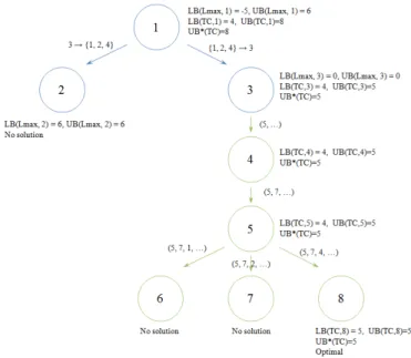
Example To illustrate algorithm B1, we consider the following example with seven jobs where the vehicle capacity c is equal to 2. Table 3 gives the jobs’ parameters.
Table 3: Example to illustrate the branch-and-bound algorithm B1 Order j 1 2 3 4 5 6 7
pj 13 18 19 20 7 8 2
rj 35 38 14 21 1 48 14
dj 69 79 99 80 65 88 51
Figure 5 illustrates the search tree of the branch-and-bound algorithm B1. At the root, i.e. node 1, since U B(Lmax, u) > 0 and LB(Lmax, u) ≤ 0, we check
U B(T C, u) and LB(T C, u). Since U B(T C, 1) = 8, i.e. the algorithm does not find a feasible NSP schedule, the algorithm branches as Carlier’s algorithm. Here, we have the critical job e = 3 and the critical set J = {1, 2, 4}.
Figure 5: Illustration of the branch-and-bound algorithm B1
At node 2, Carlier’s algorithm requires the critical job to be processed before the jobs of the critical set by setting the deadline of the critical job 3 to d3(2) =
29. Since LB(Lmax, 2) = 6 and U B(Lmax, 2) = 6, the algorithm ensures that
there is no feasible NSP-NSD schedule for node 2.
At node 3, Carlier’s algorithm requires the critical job to be processed after the jobs of the critical set by setting the release date of the critical job 3 to r3(3) = 72. Since LB(Lmax, 3) = 0 and U B(Lmax, 3) = 0, the algorithm ensures
that there is at least one feasible NSP-NSD schedule. Then it applies algorithm B2. The precedence relations include that the job 3 has to be processed after the jobs 1, 2 and 4. Since initially LB(T C, 3) = 4 and U B(T C, 3) = 5, the branching is performed as prescribed by algorithm B2. U B∗(T C) is updated to 5.
For the first position of production schedule, algorithm B2 finds that job 5 is the only job that respects the rules among the candidates. By scheduling job 5 in the first position, node 4 is generated. Since rk(3) < r5(3) + p5(3), ∀k ∈ N \{5},
the algorithm does not change the release dates. Since LB(T C, 4) = 4 and U B(T C, 4) = 5, the tree continues to branch. We still have U B∗(T C) = 5.
The algorithm finds the only candidate 7 for the second position of produc-tion schedule. By scheduling job 7 in the second posiproduc-tion, node 5 is generated. Since rk(4) < r7(4) + p7, ∀k ∈ N \{5, 7}, the algorithm does not change the
release dates. Since LB(T C, 5) = 4 and U B(T C, 5) = 5, the tree continues to branch. We still have U B∗(T C) = 5.
For the third position of production schedule, algorithm B2 finds a set of candidates {1, 2, 4}.
By scheduling job 1 in the third position, node 6 is generated. The algorithm sets r2(6) = max{r2(5), r1(5) + p1} = 48 and r4(6) = max{r4(5), r1(5) + p1} =
48. With this modified setting, there is no feasible solution for SP-NSD prob-lem in the two special cases. Hence there is no feasible solution for NSP-NSD problem.
By scheduling job 2 in the third position, node 7 is generated. The algorithm sets r1(7) = max{r1(5), r2(5) + p2} = 56 and r4(7) = max{r4(6), r2(6) + p2} =
56. With this modified setting, there is no feasible solution for SP-NSD prob-lem in the two special cases. Hence there is no feasible solution for NSP-NSD problem.
By scheduling job 4 in the third position, node 8 is generated. The algorithm sets r1(8) = max{r1(5), r4(5) + p4} = 41 and r2(8) = max{r2(5), r4(5) + p4} =
41. With this modified setting, algorithm B1 computes LB(T C, 8) = 5 and U B(T C, 8) = 5, a local optimal solution is found. Since there is no active node, the algorithm stops and an global optimal solution for NSP-NSD problem is found (see figure 6).
Figure 6: An optimal solution for NSP-NSD problem
pro-duction sequence is (5, 7, 4, 1, 2, 6, 3). There are five delivery batches: {7}, {5, 1}, {2}, {4, 6}, and {3}, which depart respectively at time 16, 54, 72, 80, and 99.
4.2.3 Mixed integer linear programming model
Lemma 5. There exists an optimal integrated schedule for NSP-NSD problem, such that each batch is delivered at one delivery deadline of job.
Proof. Suppose that there is an optimal integrated schedule for NSP-NSD prob-lem that does not satisfy the property. We can change the delivery time of each batch to satisfy the property without changing the number of delivery batches.
We propose a MILP model which extends the time-indexed scheduling model as follows. We note that {minj∈Nrj, minj∈Nrj+ 1, . . . , min(maxi∈Nri+
P
i∈Npi, maxi∈Ndi)} is the set of possible production starting times. Let T
denote this set. In this model, according to Lemma 5, we can suppose that each delivery batch departs at one job deadline. Note that one batch departs at a delivery deadline of job (which can be out of this batch) between the last production completion time of jobs in this batch and the earliest deadline of jobs in this batch. Let s1, . . . , su denote the possible delivery batch departure
dates. Decision variables: • xit=
1, if production job i starts at time t, i ∈ {1, . . . , n}, t ∈ T 0, otherwise • yiq=
1, if job i is delivered at time sq,
i ∈ {1, . . . , n}, q ∈ {1, . . . , u} 0, otherwise
• wq= number of batches departing at time sq, q ∈ {1, . . . , u}
MILP: min u X q=1 wq (7) s.t. X t∈T xit= 1, i ∈ {1, . . . , n} (8) n X i=1 t X k=max{ri,t+1−pi} xik≤ 1, t ∈ T (9) xit= 0, i ∈ {1, . . . , n}, t < ri or t > di− pi (10)
X t∈T txjt+ pj≤ u X q=1 (yjqsq), j ∈ {1, . . . , n} (11) n X i=1 yiq≤ cwq, q ∈ {1, . . . , u} (12) u X q=1 yiq= 1, i ∈ {1, . . . , n} (13) yiq= 0, i ∈ {1, . . . , n}, q ∈ {1, . . . , u}, di< sq (14) yiq∈ {0, 1}, i ∈ {1, . . . , n}, q ∈ {1, . . . , u} (15) wq ∈ N, q ∈ {1, . . . , u} (16) xit∈ {0, 1}, i ∈ {1, . . . , n}, t ∈ T (17)
In MILP, the objective function is to minimize the transportation cost. Con-straints (8) ensure that any job i starts its processing once. ConCon-straints (9) guarantee that the interval [t, t + 1], for each t, is occupied by at most one job. The interval [t, t + 1] is occupied by job i only if job i starts its processing in the interval [max{ri, t + 1 − pi}, t]. Constraints (10) ensure that job i starts
its processing in the interval [ri, di− pi]. Constraints (11) ensure that each job
is delivered after or at its production completion time. Constraints (12) are the batch capacity constraints. Constraints (13) ensure that each job is deliv-ered in one batch only. Constraints (14) are the delivery deadlines constraints. Constraints (15)-(17) give the domain of definition of each variable.
5
Computational results
In this section, we evaluate the performance of the branch-and-bound algo-rithm B1 by comparing it with MILP. The branch-and-bound algoalgo-rithm is im-plemented in C++ and the MILP model is imim-plemented in Cplex V12.1. The experiments are carried out on a DELL 2.50GHz personal computer with 8GB RAM.
We reuse the method of Briand et al. (2010) to generate instances. We consider n ∈ {10, 20, 30, 50, 70, 100, 150, 200, 300, 500}. The integers pj, rj
and dj are generated respectively from the uniform distributions [1,50], [0,
αPn j=1pj] and [(1 − β)aP n j=1pj, aP n j=1pj], where α, β ∈ {0.2, 0.4, 0.6, 0.8, 1}
and a ∈ {100%, 110%}. If dj < rj+ pj, dj has been updated by rj+ pj. The
transportation cost of one batch is equal to 1. We choose a set of hard instances as follows: we apply the branch-and-bound algorithm of Carlier to find the min-imum Lmaxfor each instance, if the problem for this instance cannot be solved
at the root of the search tree, we consider this instance as a hard instance. If the found Lmaxof this hard instance is positive, we add this value to each dj of this
instance to ensure that we have at least one feasible solution. For n ≤ 70, we consider the batch capacity c ∈ {2, 3, dn8e, dn
4e}, and c ∈ {d n 50e, d n 30e, d n 20e, d n 10e}
for n ≥ 100. 80 hard instances for each value of n are generated. Totally 800 hard instances are generated.
Table 4: Performance of the branch-and-bound algorithm B1.
n Fea Opt Node Time 10 100% 100% 2 0.07 20 100% 100% 16 0.85 30 100% 96.25% 165 14.82 50 100% 95% 173 19.16 70 100% 91.25% 183 36.13 100 100% 77.5% 324 78.46 150 100% 66.25% 334 118.18 200 100% 51.25% 298 150.02 300 100% 32.5% 240 209.01 500 100% 32.5% 118 212.98
Table 5: Performance of MILP.
n Fea Opt Node Time 10 100% 100% 1 0.87 20 100% 100% 313 12.14 30 100% 78.75% 1401 108.64 50 96.25% 37.5% 357 215.86 70 75% 27.5% 98 264.52
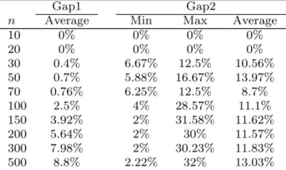
Table 6: Gaps of solutions of the branch-and-bound algorithm B1.
Gap1 Gap2
n Average Min Max Average 10 0% 0% 0% 0% 20 0% 0% 0% 0% 30 0.4% 6.67% 12.5% 10.56% 50 0.7% 5.88% 16.67% 13.97% 70 0.76% 6.25% 12.5% 8.7% 100 2.5% 4% 28.57% 11.1% 150 3.92% 2% 31.58% 11.62% 200 5.64% 2% 30% 11.57% 300 7.98% 2% 30.23% 11.83% 500 8.8% 2.22% 32% 13.03%
Tables 4 - 7 illustrate the performance of branch-and-bound algorithm B1. Imposing 5 minutes as the limit of execution time, we use the following measures to compare the branch-and-bound algorithm with the MILP model.
Fea: the percentage of instances for which a feasible solution is determined within the given time.
Table 7: Gaps of solutions of MILP.
Gap1 Gap2
n Average Min Max Average 10 0% 0% 0% 0% 20 0% 0% 0% 0% 30 5.61% 6.25% 62.5% 26.4% 50 22.79% 3.85% 86.75% 37.34% 70 37.95% 6.67% 90.96% 59.92%
Opt: the percentage of instances which are solved to optimality within the given time.
Node: the average number of explored nodes. Time: the average CPU time in seconds.
Gap1: the relative gap measured by (U B∗(T C) − LB∗(T C))/LB∗(T C), where U B∗(T C) and LB∗(T C) are the best upper bound and lower bound. We
consider the instances for which we obtained at least one feasible solution (optimal solution included).
Gap2: the relative gap for the instances for which we obtained at least one feasible solution (optimal solution excluded).
The results show that the branch-and-bound algorithm B1 outperforms the MILP model. From Tables 4 - 5, we observe that the average execution time and the number of nodes with the MILP model are always larger than the branch-and-bound algorithm. MILP cannot find a feasible solution with n ≥ 100. The branch-and-bound algorithm solves all instances with n ≤ 20 optimally within a very short execution time less than one second, and more than 90% of instances with n ≤ 70 within an average execution time less than 40 seconds. The branch-and-bound algorithm finds at least a feasible solution and solve 32.5% of instances optimally with n up to 500 and 5 minutes as time limit.
Consulting the gaps in Tables 6 - 7, we observe that the branch-and-bound algorithm has a much better performance. In average, Gap1 and Gap2 of the branch-and-bound algorithm are less than 0.8% and 14% when n ≤ 70. How-ever, the maximum Gap2 shows some hard cases for the branch-and-bound algorithm when n ≥ 100. For the MILP model, in average, Gap1 and Gap2 exceed 20% and 30% respectively when n = 50.
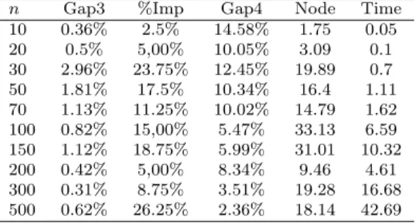
When the number of jobs is very large, it is difficult to construct a simple heuristic that guarantees that a feasible solution is found (especially when dead-lines are tight). For this reason, for large instances, the B&B algorithm could be stopped after a fixed amount of time and/or when a first feasible solution is found. We report in Table 8 the results when a first feasible solution is found. We use the following measures.
Gap3: average gap between the cost of the final solution of the B&B (computa-tional times limited to 5 minutes) and the first obtained feasible solution.
Table 8: Results of the first feasible solution obtained by the branch-and-bound algorithm
n Gap3 %Imp Gap4 Node Time 10 0.36% 2.5% 14.58% 1.75 0.05 20 0.5% 5,00% 10.05% 3.09 0.1 30 2.96% 23.75% 12.45% 19.89 0.7 50 1.81% 17.5% 10.34% 16.4 1.11 70 1.13% 11.25% 10.02% 14.79 1.62 100 0.82% 15,00% 5.47% 33.13 6.59 150 1.12% 18.75% 5.99% 31.01 10.32 200 0.42% 5,00% 8.34% 9.46 4.61 300 0.31% 8.75% 3.51% 19.28 16.68 500 0.62% 26.25% 2.36% 18.14 42.69
%Imp: average percentage of instances where the two solutions are different. Gap4: average gap between the cost of the final solution of the B&B and the
first obtained feasible solution, for instances where they are different. The results show that good solutions can be found for large instances within a reasonable amount of computational time (43 seconds in average for n = 500). The relative gap (Gap4 ) decreases when n increases, justifying the use of the B&B algorithm as a good heuristic.
6
Conclusions
In this paper, we studied an integrated production and outbound distribution scheduling problem in a supply chain with one manufacturer, and one cus-tomer. We considered a single machine production and a direct batch delivery. Moreover, we considered an important feature in production and distribution: splittable or non-splittable production/distribution. We first investigated the scheduling problems induced by the decentralized system scenario. We reviewed the production scheduling problems (i.e. SP and NSP problems) and provided two polynomial-time algorithms to solve the distribution scheduling problems (i.e. SD and NSD problems). Then we investigated the scheduling problems in the integrated system scenario (i.e. SP-NSD, SP-SD and NSP-NSD problems). We provided a polynomial algorithm to solve two special cases of SP-NSD and SP-SD problems. We also provided a branch-and-bound algorithm for NSP-NSD problem and evaluated its performance with numerical experiments. The results showed that the proposed algorithm has a better performance than the MILP model and can solve more than 90% of instances with n ≤ 70 optimally within an average execution time less than 40 seconds.
Several important research issues remain open for future investigations. A first research direction is to fix the complexity of SP-NSD and SP-SD problems. Solving one of these problems efficiently would provide a better lower bound for the branch-and-bound algorithm that solves problems NSP-NSD. A second issue is to consider the same model with a limited number of vehicles and/or
with fixed pickup times. Finally, one might consider extending the model to production systems with parallel machines.
References
[1] Averbakh, I., Xue, Z.: On-line supply chain scheduling problems with pre-emption. European Journal of Operational Research 181(1), 500 – 504 (2007)
[2] European Commission: Road Freight Transport Vademecum 2010 Report (2011)
[3] Averbakh I.: Online integrated production-distribution scheduling prob-lems with capacitated deliveries. European Journal of Operational Research 200:377384 (2010)
[4] Averbakh I., Baysan M.: Semi-online two-level supply chain scheduling problems. Journal of Scheduling 15(3):381–390 (2012)
[5] Averbakh I., Baysan M.: Approximation algorithm for the on-line multi-customer two-level supply chain scheduling problem. Operations Research Letters 41(6):710714 (2013)
[6] Averbakh I., Baysan M.: Batching and delivery in semi-online distribution systems. Discrete Applied Mathematics 161:2842 (2013)
[7] Baker, K.R., Lawler, E.L., Lenstra, J.K., Kan, A.H.G.R.: Preemptive scheduling of a single machine to minimize maximum cost subject to re-lease dates and precedence constraints. Operations Research 31(2), 381– 386 (1983)
[8] Briand, C., Ourari, S., Bouzouia, B.: An efficient ilp formulation for the single machine scheduling problem. RAIRO - Operations Research 44, 61–71 (2010)
[9] Carlier, J.: The one-machine sequencing problem. European Journal of Operational Research 11(1), 42–47 (1982)
[10] Chen, Z.L.: Integrated production and outbound distribution scheduling: Review and extensions. Operations Research 58(1), 130–148 (2010) [11] Chen, Z.L., Pundoor, G.: Integrated order scheduling and packing.
Pro-duction and Operations Management 18(6), 672–692 (2009)
[12] Condotta, A., Knust, S., Meier, D., Shakhlevich, N. V.: Tabu search and lower bounds for a combined productiontransportation problem. Comput-ers & Operations Research, 40(3), 886–900 (2013)
[13] Dror, M., and Trudeau, P.: Savings by split delivery routing. Transporta-tion Science 23(2) 141–145 (1989)
[14] Feng, X., Cheng, Y., Zheng, F., Xu, Y.: Online integrated productiondistri-bution scheduling problems without preemption. Journal of Combinatorial Optimization, DOI 10.1007/s10878-015-9841-6 (2015)
[15] Fu, B., Huo, Y., Zhao, H.: Coordinated scheduling of production and deliv-ery with production window and delivdeliv-ery capacity constraints. Theoretical Computer Science, 422, 39-51 (2012)
[16] Garey, M., Johnson, D.: Computers and Intractability: A Guide to the Theory of NP-Completeness. W.H. Freeman (1979)
[17] Gharbi, A., Haouari, M.: Minimizing makespan on parallel machines sub-ject to release dates and delivery times. Journal of Scheduling 5(4), 329–355 (2002)
[18] Graham, R.L., Lawler, E.L., Lenstra, J.K., Rinnooy Kan, A.H.G.: Opti-mization and approximation in deterministic sequencing and scheduling: a survey. In: E.J. P.L. Hammer, B. Korte (eds.) Discrete Optimization II, Annals of Discrete Mathematics, vol. 5, pp. 287–326. Elsevier (1979) [19] Hall, L.A., Shmoys, D.B.: Approximation algorithms for constrained
scheduling problems. Proc. 30th Annual Sympos. Foundations Comput. Sci. p. 134140 (1989)
[20] Hall, L.A., Shmoys, D.B.: Jackson’s rule for single-machine scheduling: Making a good heuristic better. Mathematics of Operations Research 17(1), 22–35 (1992)
[21] Hall, N., Potts, C.: The coordination of scheduling and batch deliveries. Annals of Operations Research 135(1), 41–64 (2005)
[22] Hall, N.G., Potts, C.N.: Supply chain scheduling: Batching and delivery. Operations Research 51(4), 566–584 (2003)
[23] Horn, W.A.: Some simple scheduling algorithms. Naval Research Logistics Quarterly 21(1), 177–185 (1974)
[24] Jackson, J.R.: Scheduling a production line to minimize maximum tardi-ness. Tech. rep., University of California, Los Angeles (1955)
[25] Kaminsky, P.: The effectiveness of the longest delivery time rule for the flow shop delivery time problem. Naval Research Logistics 50, 257–272 (2003)
[26] Lawler, E.L.: Optimal sequencing of a single machine subject to precedence constraints. Management Science 19(5), 544–546 (1973)
[27] Lenstra, J., Rinnooy Kan, A., Brucker, P.: Complexity of machine schedul-ing problems. In: P. Hammer, E. Johnson, B. Korte, G. Nemhauser (eds.) Studies in Integer Programming, Annals of Discrete Mathematics, vol. 1, pp. 343 – 362. Elsevier (1977)