Analysis of image series through global digital image correlation

HAL Id: hal-00694332

https://hal.archives-ouvertes.fr/hal-00694332

HAL is a multi-disciplinary open access archive for the deposit and dissemination of sci-entific research documents, whether they are pub-lished or not. The documents may come from teaching and research institutions in France or

L’archive ouverte pluridisciplinaire HAL, est destinée au dépôt et à la diffusion de documents scientifiques de niveau recherche, publiés ou non, émanant des établissements d’enseignement et de recherche français ou étrangers, des laboratoires

Analysis of image series through global digital image

correlation

Gilles Besnard, Hugo Leclerc, François Hild, Stéphane Roux, Nicolas Swiergiel

To cite this version:

Gilles Besnard, Hugo Leclerc, François Hild, Stéphane Roux, Nicolas Swiergiel. Analysis of image series through global digital image correlation. Journal of Strain Analysis for Engineering Design, SAGE Publications, 2012, 47 (4), pp.214-288. �10.1177/0309324712441435�. �hal-00694332�

Analysis of Image Series through

Global Digital Image Correlation

Gilles Besnard,

Hugo Leclerc,

Fran¸cois Hild,

St´

ephane Roux

and Nicolas Swiergiel

a

_LMT-Cachan

ENS de Cachan/CNRS/UPMC/PRES UniverSud Paris

61 avenue du Pr´

esident Wilson, F-94235 Cachan Cedex, France

b

_EADS-IW

12 rue Pasteur, F-92152 Suresnes, France

Abstract

Most often, Digital Image Correlation (DIC) is used to analyze a sequence of images. Exploitation of an expected temporal regularity in the displacement fields can be used to enhance the performances of a DIC analysis, either in terms of spatial resolution, or in terms of uncertainty. A general theoretical framework is presented, tested on artificial and experimental image series.

Keywords: Digital image correlation; displacement field; measurement

un-certainty; resolution; spatiotemporal regularization; video.

1

Introduction

In the field of solid mechanics, since the early 1980’s [1, 2, 3], most of the procedures dealing with digital image correlation (DIC) of 2D pictures (or 3D volumes) are based upon the registration of a pair of pictures, a first one corresponding to the reference configuration and the second one to the deformed configuration [4]. They consist in subdividing the region of interest in the reference picture into a set of independent zones of interest (ZOIs). The latter ones are small interrogation windows that are registered, and may overlap since there is no spatial constraint on neighboring windows. The advantage is that the analysis of each ZOI can be run independently of the other ones. The drawback is that the continuity of initially contiguous ZOIs is not obtained because of measurement uncertainties. This lack of continuity is one of the criteria used to estimate the quality of the registration [6]. This type of approach is referred to as ‘local’ in the sense that the registration is performed with small ZOIs with no information exchange with neighboring ZOIs.

The same type of approach was developed independently in the context of fluid mechanics (i.e., particle image velocimetry or PIV [5]) starting in the late 1970’s [7, 8, 9]. Very early on, regularization techniques [10, 11] were proposed [12, 13] since the gray level conservation, i.e., the underlying conservation principle to determine the optical flow, is very difficult to achieve

when using particles in a 3D flow observed with a single camera. Conversely, in solid mechanics, this hypothesis is easier to achieve when, say, spraying B/W paint onto the observed surface. One other aspect is related to the measurement uncertainties that require special attention in terms of gray level interpolation to achieve resolution on the decipixel or even centipixel range [14, 15, 16] to be applicable to situations dealing with small strains.

One way of prescribing a priori, say, continuity requirements on the dis-placement field, is to resort to global approaches of DIC. In that case, the registration is carried out over the whole region of interest (ROI). This type of analysis gives more freedom to the user in the choice of the displacement field in comparison to local approaches where the type of kinematic field is generally of low degree [17]. However, the computation time is higher. For instance, Fourier expansions of the displacement field are considered. They allow for a very robust measurement of displacement fluctuations [18], provided the non-periodic contribution is accounted for by using additional kinematic degrees of freedom [19]. Another alternative is to consider shape functions of finite element procedures [20, 21]. This type of kinematics is very useful when comparisons are sought between experimental data and nu-merical simulations. In that case, the mesh and the shape functions can be identical during the measurement and identification or validation steps [22]. Further, it was shown that the continuity requirement leads to lower dis-placement uncertainties when compared to FFT-based local approaches [23] or with bilinear interpolations [35].

Up to now, only spatial features were discussed in terms of regularization procedures. The temporal axis may also be considered. It was shown that, for

very specialized kinematics, it is possible to extract in a robust way steady state 1D and 2D velocity fields [25], a spatiotemporal velocity field when only one spatial component is considered. In the last case, the combined use of space and time kinematic bases allows the user to decrease the spatial resolution by increasing the temporal resolution to achieve similar uncertainty levels [26]. This property can be used, say, when monitoring high speed experiments for which the number of pictures can be greater than 100, or even 1,000, but the spatial definition is of the order of 10 to 100 kpixels as opposed to quasi-static experiments for which cameras have a high definition (typically greater than 10 Mpixels).

More generally, with nowadays cameras, it becomes classical to have ac-cess to more than 100, 1,000 or even more pictures. Consequently, alternative techniques to incremental approaches may be considered, as was proposed when analyzing nonlinear problems [27]. Broggiato et al. [28] proposed to use 5 consecutive pictures for global DIC and a restricted (parabolic) time

change of the displacement field. This multi-frame procedure leads to a

smoother time evolution of strain rates. It is used to have a more precise evaluation of the strain rates in the central frame (i.e., local in time).

In the following developments, a global approach in space and time is proposed. It consists in using different space-time decompositions of the

dis-placement field and in solving globally the minimization of the correlation

residuals. In Section 2, the formulation of the measurement problem is pre-sented and its practical implementation discussed. The latter is based on a ‘dyadic’ spatiotemporal decomposition. Particular features of the spatiotem-poral analysis are addressed in Section 3. Among them, the initialization

of the spatiotemporal analysis, the link with digital volume correlation. A resolution analysis shows the benefit to be expected from a spatiotemporal approach. The analysis of a tensile test on an aluminum alloy sample illus-trates the fact that time can be transformed into a loading parameter, which may not be evenly distributed over the temporal axis. Last, a high speed experiment on a composite material is analyzed in Section 4.

2

Mathematical formulation

2.1

General principle

Let us briefly review the global DIC methodology, which is further extended to the spatiotemporal framework. Readers are referred to Refs. [21, 29] for further details. The starting point of the analysis is a series of images, f (x, t) where x is the vector position, of pixel coordinates (x, y), and t the time

index. The first image is acquired at time t0. The basic assumption, called

“gray level conservation,” is expressed as

f (x + u(x, t), t) = f (x, t0) (1)

where u denotes the sought planar displacement field. The strategy used

to tackle this problem is to choose a space of trial displacement fields V, a

basis of which is denoted by ψ(x), which is expected to contain a good ap-proximation of the actual (i.e., to be determined) displacement field u(x, t). Instantaneous DIC consists in writing

v(x, t) =∑

i

where ai(t) are the unknown amplitudes (or kinematic degrees of freedom) of

the estimated displacement field v. They are obtained as the argument that minimizes a global measure (over space for a given time) of the violation of gray level conservation

u(x, t) = arg min

v ∥f(x + v(x, t), t) − f(x, t0)∥ 2

ROI (3)

evaluated over the whole Region of Interest (ROI). In this expression, the

norm∥•∥ROI is commonly chosen as its L2 variant, or the quadratic difference

between the reference image f (x, t0) and the “corrected” one at time t summed

over space.

The proposed spatiotemporal analysis consists in generalizing the previ-ous space regularization (2) to space and time. Although this methodology can straightforwardly be extended to arbitrary functions ψ(x, t), the follow-ing discussion is specialized to the particular case where space and time are separated, and hence the trial function will simply be the ‘dyadic’ product of

space ψi(x) and time ϕj(t) decompositions, namely, trial displacement fields

v are written as v(x, t) =∑ i ∑ j aijψi(x)ϕj(t) (4)

As soon as the choice of a particular representation is made, the displacement field is restricted to belong to a given space. However, this is common to all discretizations and not specific to the dyadic product form. As will be shown below, a dyadic form will be shown to be very convenient for the present implementation, and allows for faster execution speeds. Let us note that the instantaneous (i.e., image by image) analysis is a particular case of the

where images were captured in addition to the reference picture (t = t0).

Amplitudes aij are to be determined from the same problem as that written

in Equation (3) with the norm ∥ • ∥_ROI×[t0,t1] defined over the time interval

[t0, t1] corresponding to the series of pictures

aij = arg min αij f ( x +∑ i ∑ j αijψi(x)ϕj(t), t ) − f(x, t0) 2 ROI×[t0,t1] (5)

where t1 is the final time of analysis.

The actual implementation of the resolution of the nonlinear problem (5) follows exactly the footsteps proposed for global DIC approaches [21]. How-ever, the major steps are here recalled in order to highlight the benefits to be gained from the specific choice of a dyadic partition between space and time decompositions.

2.2

Practical implementation

The minimization problem is tackled by a modified Newton method, which is based on a first order Taylor-expansion of the image difference with respect to the displacement field

f (x + v(x, t), t)− f(x, t0) ≈ f(x, t) − f(x, t0) + v(x, t)· ∇f(x, t)

≈ f(x, t) − f(x, t0) + v(x, t)· ∇f(x, t0)

(6)

where the latter approximation (legitimate when the displacement correc-tion is small) allows for the computacorrec-tion of the gradient term once for all iteration steps. Taking into account the specific form of the space-time

gathers all nodal amplitudes akl is obtained [M]{a} = {b} (7) where Mijkl = ˚ ROI×[t0,t1] [ψi(x)·∇f(x, t0)]ϕj(t)[ψk(x)·∇f(x, t0)]ϕl(t) dxdt (8) and bij = ˚ ROI×[t0,t1] [ψi(x)· ∇f(x, t0)]ϕj(t)[f (x, t0)− f(x, t)] dxdt (9)

The solution to this linear system provides a displacement field v(1) _that

can be used to correct the image sequence f(1)_{(x, t) = f (x + v}(1)_{, t). The}

latter is to be used in the computation of a corrected second member {b} to

evaluate the correction of the displacement field. This loop is iterated until convergence.

The specificity of the space/time decomposition as a dyadic product is now exploited from the expression of matrix [M]. Let us introduce matrix [N] the components of which are the following integrals over the ROI

Nik =

¨

ROI

[ψi(x)· ∇f(x, t0)][ψk(x)· ∇f(x, t0)] dx (10)

that is computed only from the reference image, then [M] is expressed as

Mijkl = NikΦjl (11) with Φjl= ˆ t1 t0 ϕj(t)ϕl(t) dt (12)

It is to be noted that [N] is precisely the matrix that would be used in a standard (i.e., instantaneous) global DIC analysis. Similarly the second

member {c} reads ci(t) = ¨ ROI [ψi(x)· ∇f(x, t0)][f (x, t0)− f(x, t)] dx (13) and thus bij = ˆ t1 t0 ci(t)ϕj(t) dt (14)

is a simple weighted sum of the instantaneous second member by the chosen time functions.

In practice, gradients ∇f are evaluated as derivatives of the gray level

interpolation function. Image corrections also need an interpolation scheme since sub-pixel resolutions are sought; spline interpolations were chosen. Al-ternative choices can be made as in local DIC approaches [15].

Exact gray level conservation is in general not strictly obeyed, and this principle is often relaxed in local DIC formulations, say, by resorting to zero-mean normalized cross-correlations that amount to allowing for an affine transformation of gray level without impact on the objective functional to be minimized [4, 17]. A similar relaxation can also be implemented here. It consists in rescaling the gray levels in each element so that mean and variance of both images over each element are transformed to 0 and 1, respectively. This transformation is to be performed on the reference image (prior to the

computation of matrix [M] and vector {b}), and on the corrected deformed

images after correction. Another alternative is to consider a field of contrast and brightness that would vary from picture to picture, and would be cor-rected during the initialization procedure [29]. None of these procedures were

used and no correction was considered herein.

Although among the global DIC approaches [30, 18] a finite-element based development is the most common [20, 21], other variants exist. They may exploit analytical elastic solution (e.g., a Brazilian test [23]) or numerical solutions [31]. The discussion was not limited herein to finite element dis-cretizations because this reduction has no consequence in the temporal regu-larization. From the observed decoupling between space and time contribu-tions, different routes may be considered:

• First, a simple time decomposition using linear shape functions

span-ning over 2n images allows for a sparse matrix [M]. In that case, the shape functions are written as

ϕj(t) = φ((t− tj)/∆t) (15)

where

φ(t) = max(1− |t|/n, 0) (16)

Matrix [M] involves a coupling that is straightforwardly computed as

Φjl=            (2n2+ 1)/3n if j − l = 0 (n− 1)(n + 1)/6n if |j − l| = 1 0 if |j − l| ≥ 1 (17)

• Second, a very convenient form is encountered when the time functions

are orthogonal and normalized. In that case,

If ntdenotes the number of ϕk functions, it is observed that each

itera-tion step involves nt solutions (with the same kernel [M]) of a problem

similar to an instantaneous computation. The exploitation of the time

regularity means in practice that nt is much less than the number of

images, and hence the computation load is much less an effort than the sequential evaluation of each image. Note however that the most computationally-intensive part of the algorithm is rather the image correction than the solution to the linear systems. If each degree of freedom in the time domain is apparently decoupled from the others as far as matrix [M] is concerned, the entire problem is still to be treated simultaneously because of the correction of each image by the prede-termined displacement field.

The freedom of selecting appropriate shape functions is still quite large. Fourier series is an appealing example, yet it is to be stressed that they are not well fitted to non-periodic evolutions, and hence if the latter basis is chosen, it may be convenient to add a linear ramp function to Fourier modes to account for different initial and final states. Yet another example is given by Legendre polynomials.

In the following analyses, the spatiotemporal steps will use a spatial dis-cretization made of 4-noded spatial elements with bilinear interpolation (as in a standard Q4-DIC analysis [21]). The surface of each element is equal

to ℓ2_{. The time discretization will use linear shape functions spanning over}

defined, as would be a 3D volume element, as containing ℓ2n voxels.

3

Discussion

3.1

Initialization

It is important to comment on one difficulty of the above displacement ap-proach. It is well known that a major difficulty of DIC algorithms is to cope with large displacements or large strains. This difficulty is here of ma-jor importance as the time span of the analysis may be large, and hence so will be displacement amplitudes over the entire time interval. It is thus of importance to design a way to circumvent this difficulty that allows for an automated procedure, valid for a large class of image series. The way to address it is to design a proper initialization of the displacement field so that the remaining details to be resolved deal with moderate or small displace-ment amplitudes. Although initialization is a critical feature, it does not have to be very precise. A coarse instantaneous DIC analysis of a sampling of images is performed with few degrees of freedom, and this displacement

field, projected onto the space V × T , is used to initialize the analysis.

The “coarseness” of this initialization step is an issue that cannot be dis-cussed in general as it will depend very much on the experiment to be an-alyzed. If, for instance, the origin of the large displacements comes from a global (i.e., rigid body) translation of the field of view over the time in-terval to be studied, a very quick correlation procedure based on a single translation may be appropriate (i.e., two degrees of freedom per analyzed

image couple). This will concern the cases discussed in Section 3.4 and 4. On the contrary, if strains are very large, a multiscale approach based on a low-pass filtering of images is recommended [25]. However, in that case, it may be unnecessary to carry out the pyramidal refinement procedure down to the finest details. Thus, although more challenging, this case would still represent a small additional cost as compared to the entire analysis.

3.2

Connection with Digital Volume Correlation

It is to be noted that the above analysis could be considered as a degenerate case of global Digital Volume Correlation (DVC) [32], mapping the three dimensional space coordinate (x, y, z) onto (x, y, t), namely, the reference

volume would here be f1(x, t) = f (x, t0) (i.e., an extrusion in time of the first

image), and the deformed volume the entire stack of images f2(x, t) = f (x, t).

The 3D displacement field has to be specialized to have a zero component

along the time axis vt = 0. Hence, even if such a reduction may not provide

the most efficient implementation of the space-time approach, it may be obtained quite simply from a DVC code. When an unstructured mesh in space and time is appropriate, this reduction is an easy route to follow.

The above approach aims at measuring the displacement field from the reference image. Alternatively the same approach could be tuned to measure “velocity” fields. Velocity is here to be understood as the incremental dis-placement field between two consecutive images, separated by a time interval ∆t. To carry on the analogy with a three-dimensional problem, the reference

last one) while the deformed volume would be f2(x, t) = f (x, t + ∆t), (i.e.,

the original stack of images but the first one). This approach was followed in Ref. [26] for the specific case of 1D space and 1D time discretizations.

3.3

Benefit from time regularization

One specific feature of DIC is that the uncertainty on the measured displace-ment varies with the number of kinematic degrees of freedom, and hence with element size for a finite-element based approach [21]. The lower the number of degrees of freedom, i.e., the larger the element size, the lower the uncer-tainty level. The rationale behind this observation is that the displacements are statistical quantities whose noise susceptibility is dictated by the avail-able number of pixel per degree of freedom. Spatial regularization is a way to reduce the number of degrees of freedom by additional constraints [35]. Therefore, spatial regularization is expected to reduce the displacement un-certainty for a fixed number of spatial degrees of freedom. Alternatively, for a fixed uncertainty, this technique may offer the means to enhance the spatial resolution, i.e., to have a finer spatial mesh, if the supporting space-time ele-ment extends over longer time increele-ments. In the limit of a zero displaceele-ment, this enhancement can be compared to what is called “super-resolution”, i.e., a way to achieve sub-pixel gray level definition from a collection of images of the same scene [33].

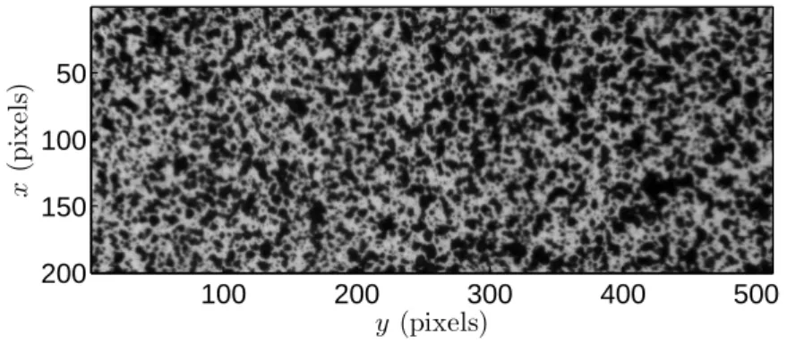
To illustrate this property, let us consider an artificial case for which the

reference picture is shown in Figure 1. Its definition is 512× 200 pixels, and

created by applying a uniform strain rate of 10−3 per picture in the

hori-zontal direction, and 5× 10−4 per picture in the vertical direction. A third

degree gray level interpolation is used herein. The spatial mesh is composed

of 16 × 16-pixel elements. Three image series are considered, namely, with

19, 49 and 99 deformed pictures in which an additional white Gaussian noise

is added with a standard deviation √2σ = 1 gray level. The maximum strain

in the longitudinal direction is equal to 2 %, 5 %, 10 % in the horizontal di-rection, and 1 %, 2.5 %, 5 % in the vertical direction. The corresponding maximum displacement is equal to 10, 25, 50 pixels in the horizontal di-rection, and 5, 12.5, 25 pixels in the vertical direction. Figure 2 shows the result in terms of mean squared error. In Figure 2(a) the results are com-pared when the deformed pictures are re-encoded as 8-bit integers and left as 64-bit floating-point numbers. There is a clear difference in terms of variance. However, the same trend is observed, namely, there is a quasi linear

varia-tion of σ2

u with the number of temporal elements. This is also true for the

second (Figure 2(b)) and third series (Figure 2(c)) for which floating-point numbers were used, irrespective of the maximum displacement and strain amplitudes. It is worth noting that the last point of each series corresponds to an instantaneous approach with the same spatial discretization as in the spatiotemporal approach.

These results can be understood by performing the following resolution analysis [21]. In the present case, it is assumed that the measurement uncer-tainties are dominated by the effect of acquisition in comparison with other uncertainties related, for instance, to gray level interpolations. It is assumed that the main cause for error is due to acquisition noise compared to gray

level interpolation. The noise-free reference being unknown, it is equivalent

to considering a noise in the difference f (x, t0)− f(x, t). The picture

differ-ence has two terms η(x, t0)− η(x, t), namely, a first one η(x, t0) of variance

σ2, and a second one, which is dependent upon the current time t, η(x, t),

with the same variance. The spatiotemporal components of η are chosen to be Gaussian and uncorrelated in space and time. Matrices [M] and [N]

are assumed to be unaffected by this noise. On the contrary, vector {c} is

modified by an increment

δcm(t) = p

∑ v

(∇f · ψm)(v){η(v, t0)− η(v, t)} (19)

whose average is thus equal to 0, and its covariance reads (when t, τ ̸= t0)

C(δcm(t), δcn(τ )) = (1 + δ(t− τ)) σ2p2Nmn (20)

where p is the physical size of one pixel. This expression shows that the

effect of noise on the spatial part at fixed time (i.e., τ = t ̸= t0) simply

consists in considering a noise of variance 2σ2 added to f (x, t) only [21].

This argument explains why a√2σ standard deviation was considered in the

previous analysis. The increment of the second member vector {b} is given

by

δbij =

∑

t

δci(t)ϕj(t) (21)

whose covariance reads

C(δbij, δbkl) = σ2p2Nik{ΦjΦl+ Φjl} (22) with Φl = ˆ t1 t0 ϕl(t) dt (23)

and Φjl given by Equation (17). The increment of the sought degrees of

freedom reads

δakl = Φ−1_jl N_ik−1δbij (24)

whose mean is vanishing since it is linearly related to that of the noise η. The corresponding covariance becomes

C(δaij, δakl) = σ2p2

{

Φ−1_jpΦpΦ−1lq Φq+ Φ−1jl

}

N_ik−1 (25)

For large values of n, Φi = n, and Φij ∝ n, hence the first term of

Equa-tion (25) is proporEqua-tional to n0 while the second term is proportional to n−1.

In addition, ∑_pΦ−1_jpΦp = 1 (independent of j apart at the ends). The

first matrix is essentially 1 for all j, l. Φ−1_jl = (1/n)Pjl where Pii ≈

√

3,

Pi,i+1 ≈ −0.46, Pi,i+2 ≈ 0.12, . . . i.e., an alternating series whose amplitude

dies off exponentially. Consequently, the first matrix plays a major role. If the correlation length (i.e., the characteristic distance over which the normalized pair correlation function decays to 0) of analyzed the texture is significantly larger than the pixel size, but not too large so that matrix [M]

is invertible, the standard displacement resolution σu reads

σu = pσ √ ⟨(∇f)2⟩ℓ √ A +B n (26)

where⟨· · ·⟩ denotes the spatial average over the considered ROI, ℓ2 the

num-ber of pixels in the considered spatial element, n the numnum-ber of pictures in

each time increment, A ≈ 1 and B dimensionless constants dependent on

the interpolation functions [21]. The result of Equation (26) when n = 1 is consistent with earlier results obtained with local [34, 35] and global [21, 35] 2D-DIC approaches. The square-root dependence with time (i.e., n) is a

direct consequence of the central limit theorem applied to image analysis for which averaging techniques are known to improve the signal to noise ratio [36].

It is worth noting that when the reference picture is noiseless, A vanishes

and σu is then inversely proportional to the square root of n

σu =

pσC

√

⟨(∇f)2⟩ℓ√_n (27)

where C is a dimensionless constant. A noiseless reference image may be more than a theoretical concept in the sense that prior to an experiment, it is possible to perform a large number of image acquisitions of the same static scene so that their average may provide such a reference image with a much smaller noise level than in the active part of the test where often time or material does not allow for such noise reduction strategies. In addition this procedure provides estimates of the noise level in the actual test conditions. This last result shows the benefit to be expected by using a time

regular-ization. For the same displacement uncertainty σu, it is possible to decrease

the spatial resolution ℓ by considering more than one image pair to perform

a correlation. When the product ℓ√n is kept constant, the standard

dis-placement uncertainty does not change. This is true provided the sought displacement field belongs to the measurement basis. This is not always the case, as will be shown in Section 4 in which the reference picture cannot be assumed noiseless. Figure 3 summarizes the results observed for the three picture series when the root mean squared difference is plotted against the time increment n used in the temporal discretization. All three series col-lapse onto a single curve that is inversely proportional to the square root of

n, as expected from Equation (27). The highest level of the standard

dis-placement resolution corresponds to an incremental analysis with the same spatial discretization.

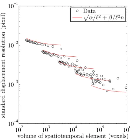
When the noiseless reference picture is unknown, the gain to be expected from the time regularization is less important (Equation 26) than previously. Figure 4 shows the results for the series of 19 pictures. The trend predicted by Equation 26) is found in the numerical results. The very small resolution levels are underestimated. Different causes may explain this deviation. One of them is related to gray level interpolations. The ratio of the two constants

A/B is found to be of the order of 1.4. Consequently, the gain of a

spa-tiotemporal analysis with a large number of pictures per time increment is

of the order of 35 % (i.e., (√A/B + 1− 1)/√A/B + 1) in terms of standard

displacement resolution when compared to an incremental approach.

3.4

Extension to time-like parameters

Up to now t was interpreted as a time parameter. However, other choices may be more appropriate. For instance, a specimen may be subjected to a mechanical test with one degree of freedom, characterized by a load, F , so that the solid remains in its linear elastic regime, and images are captured at random instants of time. In such a case, the time or image number sequence would be irrelevant. If F is used instead of t, a simple linear response is

anticipated. The substitution is straightforward for the method, and an

uneven sampling of different loads does not involve any new difficulties. Such a change of variable may however open new doors, namely, the hyperelastic

behavior of an elastomer for instance could be tackled based on a polynomial expansion in F rather than simply linear.

To illustrate this case, let us consider a tensile test on a 2024 aluminum alloy. A special setup, initially designed to test ceramics [37], was used to minimize spurious flexure when the sample is tested in the elastic regime. A long distance microscope monitors a small part of one lateral surface (i.e.,

4 mm2_{). An annular lighting was used to minimize reflectivity variations of}

the black and white paints that were sprayed onto the observed surface. A total of 22 pictures was taken when the applied load F varies between 218 and 2003 N. Figure 5 shows the reference picture (i.e., when F = 218 N).

Its definition is 1008× 1016 pixels with an 8-bit digitization. In the present

case, the pre-correction is simply a rigid body translation for each picture, and the temporal interpolation is linear since the behavior of the material is assumed to be elastic. Consequently only one time increment is considered (i.e., n = 22). Spatially, a single Q4 element is considered to capture a very simple kinematics. The main displacement gradient is obtained by spatial differentiation of the shape functions.

Two analyses are run. The first one when the reference load is F = 218 N (i.e., the minimum load level), and a second one when F = 2003 N

(i.e., the maximum load level). Figure 6 shows the convergence of the

correlation residual (i.e., √∥f(x + v(x, t), t) − f(x, t0)∥ROI×[t0,t1]/∆f , with

∆f = maxROIf (x, t0)−minROIf (x, t0)) and the maximum displacement

cor-rection as a function of the iteration number. The former tends very quickly to about 1.6 % of the dynamic range of the picture. This value provides an

The displacement corrections have an exponential decay with the number of iterations. The correlation was stopped when the value was less than

10−5 pixel. It required ten iterations of the spatiotemporal procedure. These

two results indicate that the measurements are trustworthy in both cases with about the same order of confidence.

All the results reported herein are obtained with a Core i7 (2.9 GHz)

computer. A total analysis of the 22 pictures with a 900× 900-pixel ROI,

i.e., a spatiotemporal volume of the order of 18 Mvoxels required less than

130 s of CPU time. Because a modified Newton scheme is used for all the analyses (initialization and spatiotemporal), a total of 173 (fast) iterations was needed for the initialization step. This is due to the fact that large displacements occurred in both directions (Figure 7). Conversely, the spa-tiotemporal analysis required only ten (slow) iterations because the strain

levels remained modest, i.e., at most of the order of 10−3 when expressed in

absolute values. This was possible thanks to the initialization step.

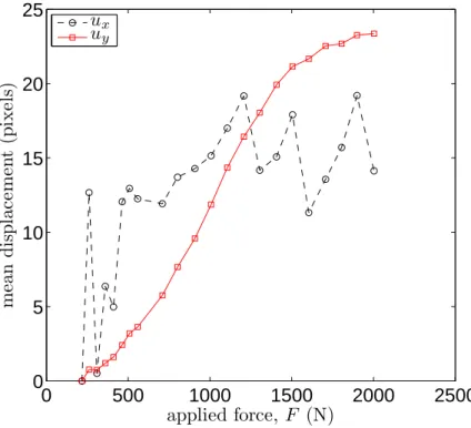
Figure 7 shows the change of the mean displacement as a function of the applied load for both directions. There is a gradual change of the

trans-verse displacement uy. In the longitudinal direction, the displacement ux is

more erratic. This is due to the fact that the long distance microscope was manually repositioned during the experiment. It is especially true at the beginning of the experiment when the sample repositions itself thanks to the elastic joint of the setup. This result shows the need for a rigid body pre-correction, picture by picture, before performing the spatiotemporal analysis. Had this pre-correction step not been implemented, low value of the correla-tion residuals could not have been reached and the spatiotemporal analysis

would have failed.

Figure 8 shows the displacement fields in the both directions for the first picture (F = 261 N) when the reference load is F = 218 N. It is worth noting that the dynamic range of the measured displacements is very small. There is a small rotation component of the same order of magnitude as the longitudinal and transverse strains. This is made possible thanks to the spa-tiotemporal analysis performed herein. By computing the mean eigen strains, it is possible to get Poisson’s ratio ν of the analyzed material. Two values are obtained, namely, ν = 0.36 when the reference picture is for F = 218 N, and ν = 0.30 when the reference picture is for F = 2003 N. Consequently, an

estimate of Poisson’s ratio is 0.33± 0.03 in very good agreement with strain

gauge measurements [38].

4

Experimental image sequence

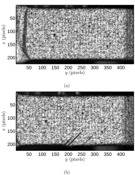
The last example treated herein corresponds to an image sequence of a tensile test on a T700 carbon fiber / M21 epoxy matrix composite with plies oriented

at±45◦ with respect to the loading direction. A high speed camera was used

to monitor the experiment with a frame rate of 65,000 fps. Consequently, the

picture definition is reduced to 224× 449 pixels (Figure 9). This is typical

of high speed experiments for which the full definition is not reachable when the frame rate increases. This is a case where the spatiotemporal analysis proposed herein is useful to have a small spatial resolution by enlarging the temporal resolution since 155 pictures are available before the final failure of the composite. However, after picture no. 100 the damage state of the

ma-terial becomes very important (Figure 9(b)). The analysis will be restricted to deformed pictures no. 1 to 99 in the sequel. The ROI is here composed of 336× 175 pixels.

4.1

Resolution analysis

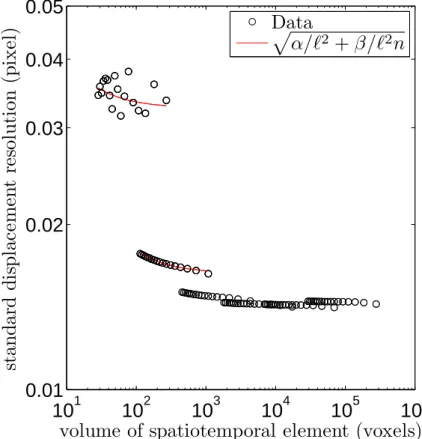
A first analysis indicates that from deformed picture no. 1 to 19 the displace-ments and strains remain vanishingly small. Consequently, a spatiotemporal analysis can be performed to assess the resolution of the technique for dif-ferent spatial and temporal discretizations. Figure 10 shows the change of the standard displacement resolution as a function of the volume of the spa-tiotemporal elements. The resolution is estimated from the values of the nodal displacements. Contrary to the artificial case, the standard resolution saturates in the centipixel range. This is presumably due to the digitization of the pictures that leads to a lower bound of the displacement resolution.

When the volume of the spatiotemporal elements is recast in terms of an equivalent length (i.e., the cube root of the volume), it is observed that the standard displacement resolution is less than 4 centipixels for element lengths greater than or equal to 5 pixels. The trend predicted by Equation (26) is obtained for the data before saturation. A good agreement is observed. The ratio of the interpolation coefficients A and B defined in Equation (26) is of the order of 0.2, thereby indicating a benefit to be expected from the spatiotemporal analysis for large time increments of the order of 10 % (i.e., (√A/B + 1− 1)/√A/B + 1) for small spatial elements, see Figure 10. This

small spatial elements are considered.

4.2

Analysis of the experiment

The experiment reported herein is deemed difficult because cracks appear during the analyzed sequence (Figure 9(b)); the hypothesis of displacement continuity in the spatial and temporal domains will be violated at the end of the sequence. Consequently, the spatial and temporal discretizations will be adapted to capture these events. A set of analyses is run with different spatial and temporal discretizations. Figure 11 shows the change of the correlation with the volume of the spatiotemporal elements. It is observed that the finest spatial discretization is needed to get the smallest correlation residual. It corresponds to spatial elements of equivalent length less than 5.4 pixels. This length can be used since the temporal axis is composed of 5 increments of 18 pictures each. In the present case, the temporal discretization does not have to be very fine. The correlation residual level is less than 3 %, which is higher than those observed in the resolution analysis (i.e., less than 1 %), but still low enough to study the measured results. This discretization is chosen for the remainder of the section.

With these parameters, the spatiotemporal volume of interest is of the order of 5.3 Mvoxels. In the present case, the initialization step was very fast and required only a few (fast) iterations for the 90 analyzed pictures. On the other hand, 20 spatiotemporal iterations were needed because of the complexity of the analyzed kinematics due to the presence of cracks. The

54 analyses with various spatiotemporal discretizations shown in Figure 11 were obtained in less than two hours. This corresponds to a cumulative spatiotemporal volume of 286 Mvoxels.

Figure 12(a) shows the change of the mean displacement in both direc-tions. The longitudinal component has a steady change with the picture number. This is not the case for the transverse displacement that starts to fluctuate, and becomes steadier from picture no. 60 on. This regime is due to the loading conditions prescribed by the high speed tensile testing ma-chine. Again, the picture by picture displacement pre-correction is needed to enable for the spatiotemporal analysis. In Figure 12(b), the mean strain components are plotted. The shear strains remain small compared to the two normal components throughout the analysis. The mean normal strain components have a smooth history, even though rigid body motions fluctuate. There are two regimes, namely a first one prior to picture no. 50, pre-sumably the elastic domain (e.g., when the first 11 pictures are used, the mean ratio of the transverse to longitudinal strains is equal to -0.78 which is in complete agreement with the values measured by strain gauges), and a second one during which the strain rate increases. This trend is due to non-linear phenomena such as multiple cracking (Figure 9(b)) as will be proven in the sequel. Since the strain gauges are not mounted on the same face, the fact that the transverse signal departs from the value evaluated from the spatiotemporal approach may be caused by the heterogeneity of the damage field. From this plot, it is deduced that the mean longitudinal strain rate

of the experiment is 43 s−1. Further, the apparent Poisson’s ratio has small

values are in very good agreement with known levels observed for this type of material [39].

The global residuals were observed to be of the order of 3 % for the an-alyzed sequence. However, the mean value per picture is not constant. Fig-ure 13 shows its change with the pictFig-ure number. The first part corresponds to displacements that are vanishingly small. Part of these pictures were an-alyzed when the resolution was assessed. There is a second regime during which the mean correlation residual is of the order of 2.4 %. It corresponds to a situation where no cracks are observed. The reason for the increase of the mean correlation residual in the third regime (i.e., after picture no. 60) is due to cracking. This last conclusion can be drawn from the analysis of the normalized residual fields shown in Figure 14. Cracks are clearly visible for the residual field corresponding to picture no. 53. Multiple cracking zones can be observed in the residual of picture no. 71. Two fully damaged zones can be seen in the residual field of picture no. 99. This analysis allows one to understand the gradual increase of the mean correlation per picture shown in Figure 13.

For the same pictures, the two components of the displacement field are shown in Figure 15. Multiple cracks are observed in the maps corresponding to picture no. 53. Their number increases with the strain level and a lot of them are present in the maps corresponding to picture no. 99. Their exact numbering is not addressed herein. The fact that numerous cracks appear explains why the mean correlation residuals gradually increase (Figure 13). This is also the reason for requiring a fine spatial discretization.

5

Conclusions

A spatiotemporal analysis was proposed to analyze a picture series with a global digital image correlation technique. By extending to the temporal axis the spatial regularization provided by a global approach (e.g., Q4-DIC [21]), it is shown that a series of pictures can be correlated by directly considering the whole sequence as opposed to an incremental approach generally performed. It is worth remembering that the spatiotemporal basis may be completed by a basis of rigid body motions that vary from picture to picture. This is important when analyzing experiments during which the first part of the loading leads to a repositioning of the sample in the testing device. This was the case of the two experiments reported herein.

A resolution analysis shows that the standard displacement uncertainty is inversely proportional to the square root of the spatiotemporal element size. This result shows the benefit to be expected from this type of approach. When the picture definition is small, as often happens when high speed cam-eras are used, it is possible to have a small spatial resolution (i.e., the element size in the spatial domain) by enlarging the temporal resolution (i.e., the time increment) to achieve the same overall measurement uncertainty. This result was validated against an artificial and a real case.

The previous result can also be used to analyze the elastic response of a material for which a linear relationship between the measured displacement and the applied load can be enforced during the measurement stage. The time axis then corresponds to the load axis with no change in the algorithm, even when the load data are not evenly distributed along the temporal axis.

It was possible to extract the Poisson’s ratio of the tested aluminum alloy whose mean value was in very good agreement with a value obtained by using strain gauge data.

The analysis of a dynamic tensile test on a composite material was also performed. Even though cracks appear during the applied load, the spa-tiotemporal analysis could be performed. The level of correlation residuals was low enough to have confidence in the measurement results. The conver-gence is slower because of discontinuities that appear at the middle of the picture sequence. The spatial and temporal discretizations had to be adapted to capture the main displacement and strain features. This was possible by analyzing the correlation residuals. The maximum mean longitudinal strain was found to be of the order of 5 % for 90 analyzed pictures.

The inherent flexibility of global spatial approaches to DIC is to be

ex-pected from the spatiotemporal approach as well. In the present paper,

bilinear spatial and linear temporal shape functions were considered. This is not a limitation. If other discretizations are to be considered, it is possible to implement them. This is in particular true for the temporal discretiza-tion that may tailored to the analyzed case as was performed with a uniform discretization in the analysis of the dynamic tensile test of the composite material. It is a straightforward perspective to implement automatic mesh generation along the temporal axis.

The finite-element based approach developed herein allows for a direct coupling with FE simulations. The measured displacements on the boundary of the spatiotemporal ROI could be prescribed to an explicit finite element analysis of the dynamic experiment. In that case, higher degree time

inter-polations may be considered. An alternative route is to measure the velocity field as was initially proposed [26] to analyze a high speed movie.

Acknowledgments

This work was funded by Agence Nationale de la Recherche under the grant ANR-2006-MAPR-0022-01 (VULCOMP Phase 1 Project).

References

[1] B. D. Lucas and T. Kanade, An Iterative Image Registration Technique with an Application to Stereo Vision, Proceedings 1981 DARPA Imaging

Understanding Workshop, (1981), 121-130.

[2] P. J. Burt, C. Yen and X. Xu, Local correlation measures for mo-tion analysis: a comparative study, Proceedings IEEE Conf. on Pattern

Recognition and Image Processing, (1982), 269-274.

[3] M. A. Sutton, W. J. Wolters, W. H. Peters, W. F. Ranson and S. R. McNeill, Determination of Displacements Using an Improved Digital Correlation Method, Im. Vis. Comp. 1 [3] (1983) 133-139.

[4] M. A. Sutton, J.-J. Orteu and H. Schreier, Image correlation for shape,

motion and deformation measurements: Basic Concepts, Theory and Applications, (Springer, New York, NY (USA), 2009).

[5] R. J. Adrian, Twenty years of particle image velocimetry, Exp. Fluids

[6] P. Vacher, S. Dumoulin, F. Morestin and S. Mguil-Touchal, Bidimen-sional strain measurement using digital images, Proceedings of the

In-stitution of Mechanical Engineers, Part C: Journal of Mechanical Engi-neering Science 213 [8] (1999) 811-817.

[7] D. B. Barker and M. E. Fourney, Measuring fluid velocities with speckle patterns, Optics Lett. 1 (1977) 135-137.

[8] T. D. Dudderar and P. G. Simpkins, Laser Speckle Photography in a Fluid Medium, Nature 270 (1977) 45-47.

[9] R. Grousson and S. Mallick, Study of flow pattern in a fluid by scattered laser light, Appl. Optics 16 (1977) 2334-2336.

[10] A. N. Tikhonov and V. Y. Arsenin, Solutions of ill-posed problems, (J. Wiley, New York (USA), 1977).

[11] P. J. Hubert, Robust Statistics, (Wiley, New York (USA), 1981).

[12] B. K. P. Horn and B. G. Schunck, Determining optical flow, Artificial

Intelligence 17 (1981) 185-203.

[13] M. Black, Robust Incremental Optical Flow , (PhD dissertation, Yale University, 1992).

[14] M. A. Sutton, S. R. McNeill, J. Jang and M. Babai, Effects of subpixel image restoration on digital correlation error estimates, Opt. Eng. 27 [10] (1988) 870-877.

[15] H. W. Schreier, J. R. Braasch and M. A. Sutton, Systematic errors in digital image correlation caused by intensity interpolation, Opt. Eng. 39 [11] (2000) 2915-2921.

[16] S. Bergonnier, F. Hild and S. Roux, Digital image correlation used for mechanical tests on crimped glass wool samples, J. Strain Analysis 40 [2] (2005) 185-197.

[17] M. Bornert, F. Br´emand, P. Doumalin, J.-C. Dupr´e, M. Fazzini, M. Gr´

e-diac, F. Hild, S. Mistou, J. Molimard, J.-J. Orteu, L. Robert, Y. Surrel, P. Vacher and B. Wattrisse, Assessment of Digital Image Correlation measurement errors: Methodology and results, Exp. Mech. 49 [3] (2009) 353-370.

[18] B. Wagne, S. Roux and F. Hild, Spectral Approach to Displacement Evaluation From Image Analysis, Eur. Phys. J. AP 17 (2002) 247-252. [19] S. Roux, F. Hild and Y. Berthaud, Correlation Image Velocimetry: A

Spectral Approach, Appl. Optics 41 [1] (2002) 108-115.

[20] Y. Sun, J. Pang, C. Wong and F. Su, Finite-element formulation for a digital image correlation method, Appl. Optics 44 [34] (2005) 7357-7363. [21] G. Besnard, F. Hild and S. Roux, “Finite-element” displacement fields

analysis from digital images: Application to Portevin-Le Chˆatelier

bands, Exp. Mech. 46 (2006) 789-803.

[22] S. Roux and F. Hild, Digital Image Mechanical Identification (DIMI),

[23] F. Hild and S. Roux, Digital image correlation: From measurement to identification of elastic properties - A review, Strain 42 (2006) 69-80. [24] F. Hild and S. Roux, Comparison of local and global approaches to

digital image correlation, to appear in Exp. Mech. (2012).

[25] S. Bergonnier, F. Hild and S. Roux, Analyse d’une cin´ematique

station-naire h´et´erog`ene, Revue Comp. Mat. Av. 13 [3] (2003) 293-302.

[26] G. Besnard, S. Gu´erard, S. Roux and F. Hild, A space-time approach

in digital image correlation: Movie-DIC, Optics Lasers Eng. 49 (2011) 71-81.

[27] P. Boisse, P. Bussy and P. Ladev`eze, A new approach in non-linear

mechanics: The large time increment method, Int. J. Num. Meth. Eng.

29 [3] (1990) 647-663.

[28] G. B. Broggiato, L. Casarotto, Z. Del Prete and D. Maccarrone, Full-Field Strain Rate Measurement by White-Light Speckle Image Correla-tion, Strain 45 [4] (2009) 364-372.

[29] F. Hild and S. Roux, Digital Image Correlation, in: Optical Methods for

Solid Mechanics, E. Hack and P. Rastogi, eds., 2012, in press.

[30] E. P. Simoncelli, Bayesian Multi-Scale Differential Optical Flow, in: Handbook of Computer Vision and Applications, B. J¨ahne, H. Haussecker and P. Geissler, eds., (Academic Press, 1999), 2 297-422.

[31] H. Leclerc, J.-N. P´eri´e, S. Roux and F. Hild, Integrated digital image

2009 , A. Gagalowicz and W. Philips, eds., (Springer, Berlin, 2009),

LNCS 5496 161-171.

[32] S. Roux, F. Hild, P. Viot and D. Bernard, Three dimensional image correlation from X-Ray computed tomography of solid foam, Comp. Part

A 39 [8] (2008) 1253-1265.

[33] F. Humblot and A. Mohammad-Djafari, Super-Resolution using hid-den Markov model and Bayesian Detection Estimation Framework,

EURASIP J. Appl. Signal Proc. 2006 [36971] (2006) 16 p.

[34] Y. Q. Wang, M. A. Sutton, H. A. Bruck and H. W. Schreier, Quantita-tive Error Assessment in Pattern Matching: Effects of Intensity Pattern Noise, Interpolation, Strain and Image Contrast on Motion Measure-ments, Strain 45 (2009) 160-178.

[35] F. Hild and S. Roux, Comparison of local and global approaches to digital image correlation, Exp. Mech. [submitted for publication] (2012). [36] P. Billingsley, Probability and Measure, third ed., (Wiley, New York, NY

(USA), 1995).

[37] F. Hild, E. Amar and D. Marquis, Stress Heterogeneity Effect on the Strength of Silicon Nitride, J. Am. Ceram. Soc. 75 [3] (1992) 700-702.

[38] S. Avril, M. Bonnet, A.-S. Bretelle, M. Gr´ediac, F. Hild, P. Ienny, F.

Latourte, D. Lemosse, S. Pagano, E. Pagnacco and F. Pierron, Overview of identification methods of mechanical parameters based on full-field measurements, Exp. Mech. 48 [4] (2008) 381-402.

[39] P. Th´evenet and N. Swiergiel, VULCOMP final report, (EADS IW, 2010).

Appendix: Notations

ai, unknown spatial degree of freedom

aij, {a} unknown spatiotemporal degree of freedom, vector gathering all unknowns aij

bij, {b} error component, vector gathering all components bij

ci, {c} instantaneous error component, vector gathering all components cj

f , f1, f2 series of pictures, stack of pictures in the reference and deformed configurations

f(1) _{corrected image by the estimated displacement field v}(1) _{at iteration step 1}

ℓ2 _{number of pixels in each spatial element}

ℓ2_{n number of voxels in each spatiotemporal element}

n number of pictures in each time increment

nt number of ϕk functions

p physical size of one pixel

t, tj time indices

t0, t1 initial and final time

u sought displacement field

v estimated displacement field

vt displacement component along time axis

x vector position of pixel coordinates (x, y)

z additional spatial coordinate for a 3D analysis

A, B, C constants

C(., .) covariance

F applied load

Nik spatial component of matrix [M]

Pij auxiliary matrix

V space of trial displacement field

V × T spatiotemporal space of trial displacement field

αij estimated spatiotemporal degree of freedom

δ(.) Dirac function

δij Kronecker delta

η noise component at the pixel level

ψ basis of space V

φ temporal shape function

ψj element of spatial basis

ϕk element of temporal basis

σ standard deviation of noise

σu standard displacement resolution

τ time index

∆f dynamic range of the picture in the reference configuration

∆t time difference between two consecutive pictures

Φl time integral of ϕl

Φjl temporal component of matrix [M]

∇f spatial gradient

⟨.⟩ volume average

List of Figures

1 Reference picture of the resolution analysis. . . 39

2 Resolution analysis for different numbers of deformed pictures.

Displacement variance σ2

u as a function of the number of

tem-poral elements. A quasi linear trend is observed for all

ana-lyzed cases. . . 40

3 Standard Displacement resolution σu as a function of the time

increment n for the three series analyzed in Figure 2. The

solid line corresponds to the trend predicted by Equation (27). 41

4 Standard Displacement resolution σu as a function of the

spa-tiotemporal volume ℓ2_{n for a series 19 pictures. The solid line}

corresponds to the trend predicted by Equation (26). . . 42

5 Reference picture of the tensile test on aluminum alloy (F =

218 N). . . 43

6 Convergence study. Correlation residual (a) and maximum

displacement correction (b) as functions of the iteration

num-ber. The iterations were stopped when the 10−5-pixel limit

was reached by the maximum displacement correction. . . 44

7 Mean displacements versus applied load level when the

refer-ence picture is chosen for F = 218 N. Almost identical results are observed when the reference picture is chosen for F = 2003 N. 45

8 Vertical (a) and horizontal (b) displacement fields (expressed

in pixels) for the first analyzed picture (F = 261 N) with

9 Reference picture (a) and 99th deformed picture (b) of the tensile test on a composite material. Cracks are clearly visible

on the lower edge of the sample in its deformed configuration. 47

10 Resolution analysis of the tensile test on a composite material.

Log-log plot of the standard displacement resolution as a

func-tion of the volume ℓ2n of the spatiotemporal elements. The

interpolation (solid line) described by Equation (26) is used

only for the two series that do not saturate. . . 48

11 Correlation residual as a function of the volume ℓ2_{n of}

spa-tiotemporal elements when 90 pictures are analyzed. A

mini-mum value is observed when n = 5. . . . 49

12 Mean displacements (a) and strains (b) versus picture number

for the analyzed sequence. Comparison of mean strain data measured by gauges and the spatiotemporal approach (ST-DIC). 50

13 Correlation residual per picture for the analyzed sequence. . . 51

14 Correlation residual maps at the end of the five time

incre-ments. The residuals are drawn in the deformed configuration 52

15 Vertical (left) and horizontal (right) displacement maps (in

y(pixels) x (p ix el s) 100 200 300 400 500 50 100 150 200

0 5 10 15 20 0 1 2 3 4 5x 10 −5

number of temporal elements

σ 2 u (p ix el 2) int float

(a) 19 deformed pictures

0 10 20 30 40 50 0 0.5 1 1.5 2 2.5x 10 −5

number of temporal elements

σ 2 u (p ix el 2) (b) 49 deformed pictures 0 20 40 60 80 100 0 0.5 1 1.5 2 2.5x 10 −5

number of temporal elements

σ 2 u (p ix el 2) (c) 99 deformed pictures

Figure 2: Resolution analysis for different numbers of deformed pictures.

Displacement variance σ2

u as a function of the number of temporal elements.

100 101 102

10−4

10−3

10−2

time increment, n (number of pictures)

σu (p ix el ) data B/√n

Figure 3: Standard Displacement resolution σu as a function of the time

in-crement n for the three series analyzed in Figure 2. The solid line corresponds to the trend predicted by Equation (27).

10

10

10

10

10

10

10

10

10

volume of spatiotemporal element (voxels)

st

an

d

ar

d

d

is

p

lac

eme

n

t

re

sol

u

ti

on

(p

ix

el

)

Data

pα/ℓ

_{+ β/ℓ}

_n

Figure 4: Standard Displacement resolution σu as a function of the

spa-tiotemporal volume ℓ2n for a series 19 pictures. The solid line corresponds

y (pixels) x (p ix el s) 200 400 600 800 1000 100 200 300 400 500 600 700 800 900 1000

0 2 4 6 8 10 0.015 0.016 0.017 0.018 0.019 0.02 0.021 0.022 number of iterations c o r r e lat ion r e s id u al F = 218 N F = 2003 N (a) 0 2 4 6 8 10 10−6 10−5 10−4 10−3 10−2 10−1 100 number of iterations ma x im u m d is p la ce me n t cor re ct io n (p ix el ) F = 218 N F = 2003 N (b)

Figure 6: Convergence study. Correlation residual (a) and maximum dis-placement correction (b) as functions of the iteration number. The iterations

were stopped when the 10−5-pixel limit was reached by the maximum

0 500 1000 1500 2000 2500 0 5 10 15 20 25 applied force, F (N) me an d is p lac eme n t (p ix el s) u x u y

Figure 7: Mean displacements versus applied load level when the reference picture is chosen for F = 218 N. Almost identical results are observed when the reference picture is chosen for F = 2003 N.

y(pixels) x (p ix el s) 200 400 600 800 100 200 300 400 500 600 700 800 900 12.66 12.665 12.67 12.675 12.68 12.685 12.69 (a) ux y(pixels) x (p ix el s) 200 400 600 800 100 200 300 400 500 600 700 800 900 0.76 0.765 0.77 0.775 (b) uy

Figure 8: Vertical (a) and horizontal (b) displacement fields (expressed in pixels) for the first analyzed picture (F = 261 N) with respect to the reference picture (F = 218 N).

y (pixels) x (p ix el s) 50 100 150 200 250 300 350 400 50 100 150 200 (a) y (pixels) x (p ix el s) 50 100 150 200 250 300 350 400 50 100 150 200 (b)

Figure 9: Reference picture (a) and 99th _{deformed picture (b) of the tensile}

test on a composite material. Cracks are clearly visible on the lower edge of the sample in its deformed configuration.

10

10

10

10

10

10

0.01

0.02

0.03

0.04

0.05

volume of spatiotemporal element (voxels)

st

an

d

ar

d

d

is

p

lac

eme

n

t

re

sol

u

ti

on

(p

ix

el

)

Data

pα/ℓ

_{+ β/ℓ}

_n

Figure 10: Resolution analysis of the tensile test on a composite material. Log-log plot of the standard displacement resolution as a function of the

volume ℓ2_{n of the spatiotemporal elements. The interpolation (solid line)}

102 104 106 108 0.025 0.03 0.035 0.04 0.045 0.05

volume of spatiotemporal element (voxels)

co rr el at ion re si d u al

Figure 11: Correlation residual as a function of the volume ℓ2_{n of}

spatiotem-poral elements when 90 pictures are analyzed. A minimum value is observed when n = 5.

0 20 40 60 80 100 −30 −25 −20 −15 −10 −5 0 picture number me an d is p lac eme n t (p ix el s) u_x u_y (a) 0 20 40 60 80 100 −0.06 −0.04 −0.02 0 0.02 0.04 0.06 picture number me an st ra in (-) ǫ_xx(gauge) ǫyy(gauge) ǫ_xx(ST-DIC) ǫ_yy(ST-DIC) ǫ_xy(ST-DIC) (b)

Figure 12: Mean displacements (a) and strains (b) versus picture number for the analyzed sequence. Comparison of mean strain data measured by gauges and the spatiotemporal approach (ST-DIC).

0 20 40 60 80 100 0 0.01 0.02 0.03 0.04 0.05 0.06 picture number c o rr e lat ion re si d u al

y(pixels) x (p ix el s) 100 200 300 400 50 100 150 200 0 0.2 0.4 0.6 0.8 1

(a) picture no. 27

y(pixels) x (p ix el s) 100 200 300 400 50 100 150 200 0 0.2 0.4 0.6 0.8 1 (b) picture no. 35 y(pixels) x (p ix el s) 100 200 300 400 50 100 150 200 0 0.2 0.4 0.6 0.8 1 (c) picture no. 53 y(pixels) x (p ix el s) 100 200 300 400 50 100 150 200 0 0.2 0.4 0.6 0.8 1 (d) picture no. 71 y(pixels) x (p ix el s) 100 200 300 400 50 100 150 200 0 0.2 0.4 0.6 0.8 1

(e) picture no. 99

Figure 14: Correlation residual maps at the end of the five time increments. The residuals are drawn in the deformed configuration

y(pixels) x (p ix el s) 100 150 200 250 300 350 400 50 100 150 200 1.5 2 2.5 3 y(pixels) x (p ix el s) 100 150 200 250 300 350 400 50 100 150 200 −2 −1.5 −1

(a) picture no. 27

y(pixels) x (p ix el s) 100 150 200 250 300 350 400 50 100 150 200 1 2 3 y(pixels) x (p ix el s) 100 150 200 250 300 350 400 50 100 150 200 −11 −10 −9 −8 (b) picture no. 35 y(pixels) x (p ix el s) 100 150 200 250 300 350 400 50 100 150 200 0 1 2 3 y(pixels) x (p ix el s) 100 150 200 250 300 350 400 50 100 150 200 −18 −16 −14 −12 (c) picture no. 53 y(pixels) x (p ix el s) 100 150 200 250 300 350 400 50 100 150 200 −2 0 2 4 6 8 y(pixels) x (p ix el s) 100 150 200 250 300 350 400 50 100 150 200 −25 −20 −15 (d) picture no. 71 y(pixels) x (p ix el s) 100 150 200 250 300 350 400 50 100 150 200 −5 0 5 10 15 y(pixels) x (p ix el s) 100 150 200 250 300 350 400 50 100 150 200 −35 −30 −25 −20 −15 −10

(e) picture no. 99