Approximating the performance of a last mile transportation system

Approximating the Performance of a Last Mile

Transportation System

By

Hai Wang

Bachelor of Science, Tsinghua University, 2009

Submitted to Sloan School of Management, and Department of Civil and Environmental

Engineering, in Partial Fulfillment of the Requirements for the Degrees of

Master of Science in Operations Research and

Master of Science in Transportation

at the

MASSACHUSETTS INSTITUTE OF TECHNOLOGY

June 2012

0 2012 Massachusetts Institute of Technology. All Rights Reserved.

Signature of A uthor...

.

..

. .. ...

Operations Research Center

Department of Civil & Environmental Engineering

May 16th, 2012

C ertified by ...

...

Amedeo R. Odoni

Professor of Aeronautics and Astronautics & Civil and Environmental Engineering

Thesis Supervisor

A ccepted by ...

Patrick Jaillet

A ccepted by ...

Heidi 1\. Nepf

Approximating the Performance of a Last Mile Transportation System

By

Hai Wang

Submitted to Sloan School of Management, and Department of Civil and Environmental

Engineering,

on May 16th, 2012 in Partial Fulfillment of the Requirements for the Degrees of Master

of Science in Operations Research and Master of Science in Transportation

Abstract

The Last Mile Problem (LMP) refers to the provision of travel service from the nearest

public transportation node to a home or office. We study the supply side of this problem

in a stochastic setting, with batch demands resulting from the arrival of groups of

passengers at rail stations or bus stops who request last-mile service. Closed-form bounds

and approximations are derived for the performance of Last Mile Transportations

Systems as a function of the fundamental design parameters of such systems. An initial

set of results is obtained for the case in which a fleet of vehicles of unit-capacity provides

the Last Mile service and each delivery route consists of a simple round-trip between the

rail station and bus stop and the single passenger's destination. These results are then

extended to the general case in which the capacity of a vehicle is an arbitrary, but

typically small (under 10) number. It is shown through comparisons with simulation

results, that a particular strict upper bound and an approximate upper bound, both derived

under similar assumptions, perform consistently and remarkably well for the entire

spectrum of input values and conditions simulated. These expressions can therefore be

used for the preliminary planning and design of Last Mile Transportation Systems,

especially for determining approximately resource requirements, such as the number of

vehicles/servers needed to achieve some pre-specified level of service.

Thesis Supervisor: Amedeo R. Odoni

Title: Professor of Aeronautics and Astronautics & Civil and Environmental

Engineering

Acknowledgements

First and foremost, I would like to express my great and sincere appreciation to my advisor Professor Amedeo Odoni. For the last three years, you are the constant source of knowledge, guidance and encouragement for me; you provide me continuous support and endless help all the time. I am significantly benefited from your immerse knowledge, kindly help, inspiration and patience. You are the greatest Professor and mentor I have ever met or known, and I always feel I am so lucky to be your student and work with you. Throughout the research, you provide me sound advice, lots of new ideas, tremendous guidance, and you even helped me with my languages and writing. I could not imagine a better advisor and mentor than you. I really appreciate it.

Also, I would like to thank my parents, my father Zhengqing Wang and my mother Suqing Xu, although you cannot read this acknowledgement in English. You provide the endless support and love all the time. Then years ago, who could imagine your son study and do research in Massachusetts Institute of Technology? I cannot make it without you.

Contents

L ist of F igures ... 11

L ist of T ab les ... 13

1. Problem Introduction, Description, Assumptions and Overall Approach...15

1.1 Introduction and Literature Survey...15

1.2 Problem Description and Assumptions ... 18

1.3 Description of Overall Approach...20

2. The Unit-Capacity, Multi-Vehicle LMP ... 25

2.T*: Background Results ... 26

2.1 A Lower Bound... .... 27

2.1.T1*: Lower Bound of Unit-Capacity, Multi-Vehicle LMP in the general case ... 28

2.1.T2*: Service time distribution in a rectangular service region...30

2. 1.T3*: Lower Bound of the Unit-Capacity, Multi-Vehicle LMP for a Poison customer batch size and a square service region... 31

2.2 Two Upper Bounds...32

2.2.T*: Upper bound for the average waiting time in the DN/G/1/oo queue model...33

2.2.1 Randomized Assignment Policy... 36

2.2.1.T1*: Upper bound of the Unit-Capacity, Multi-Vehicle LMP under randomized assignment policy in the general case... 37

2.2. 1.T2*: Upper bound of the Unit-Capacity, Multi-Vehicle LMP under randomized assignment policy for a Poisson customer batch size and a square service region... 38

2.2.2 Cyclic Assignment Policy... 41

2.2.2.T1*: Upper bound of the Unit-Capacity, Multi-Vehicle LMP under cyclic assignment policy in the general case... 42

2.2.2.T2*: Upper bound of the Unit-Capacity, Multi-Vehicle LMP under cyclic assignment policy for a Poisson customer batch size and a square service region... 44

2.2.2.T3*: Upper bound of the Unit-Capacity, Multi-Vehicle LMP under cyclic assignment

policy for a Poisson customer batch size and a square service region when m/i is large ....47

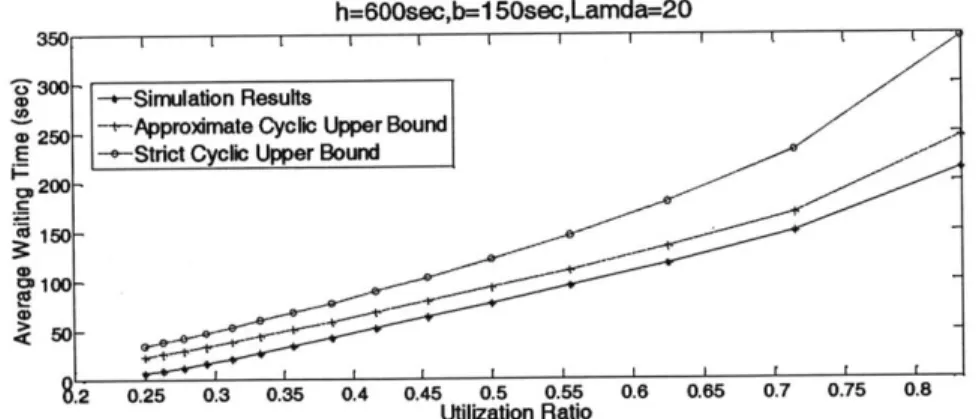
2.3 Numerical Experiments for the Unit-Capacity, Multi-Vehicle LMP...50

2.4 Sensitivity Analysis: Unit-Capacity, Multi-Vehicle LMP ... 53

2.4.1 Rectangular Service Region (a = kb, k > 1)...53

2.4. 1.T*: Sensitivity analysis of Unit-Capacity, Multi-Vehicle LMP for rectangle service region with length a and width b (a = kb, k > 1)...55

2.4.2 Diamond Service Region with Side of Length b... 60

2.4.2.T*: Sensitivity analysis of Unit-Capacity, Multi-Vehicle LMP for diamond service region w ith side b...62

2.4.3 Rectangular Service Region with Barrier ... 67

2.4.3.T*: Sensitivity analysis of Unit-Capacity, Multi-Vehicle LMP for rectangle service region w ith barrier...68

3. General-Capacity, Multi-Vehicle LMP: Upper Bounds and Approximations...77

3.1 Approximating the Expectation and Variance of Tour Lengths...77

3.1.T1*: Expectation and variance for first leg under greedy routing strategy...80

3.1.T2*: Expectation and variance for last leg under greedy routing strategy...83

3.1.T3*: Expectation and variance approximation for middle leg using Crofton's method..85

3. 1.T4*: Expectation and variance approximation for middle leg using Center approximation m ethod ... 93

3.1.T5*: Regression correction for middle leg approximations... 93

3.2 Completion of the Queuing Model... 97

3.2.T*: Upper bound and approximation of the General-Capacity, Multi-Vehicle LMP under cyclic assignm ent policy... 99

3.3 Simulation and Comparisons for the General-Capacity, Multi-Vehicle LMP...104

3.3.T*: Accuracy evaluation of Travelling Salesman Problem (TSP) heuristic algorithm used in the num erical experim ent ... 105

4. Conclusion...111

List of Figures

Figure 1: Schematic of a Last Mile Transportation System (LMTS)... 15

Figure 2: Customer destinations and vehicles routes of the Unit-Capacity, Multi-Vehicle LMP .21 Figure 3: Vehicle routes of the General-Capacity, Multi-Vehicle LMP... 22

Figure 4: Customer flow in the pre-assignment policy...32

Figure 5: Randomized assignment policy... 36

Figure 6: Cyclic assignm ent policy ... 41

Figure 7: Simulation results and cyclic upper bounds of average waiting time when A = 20...50

Figure 8: Simulation results and cyclic upper bounds of average waiting time when A = 40...50

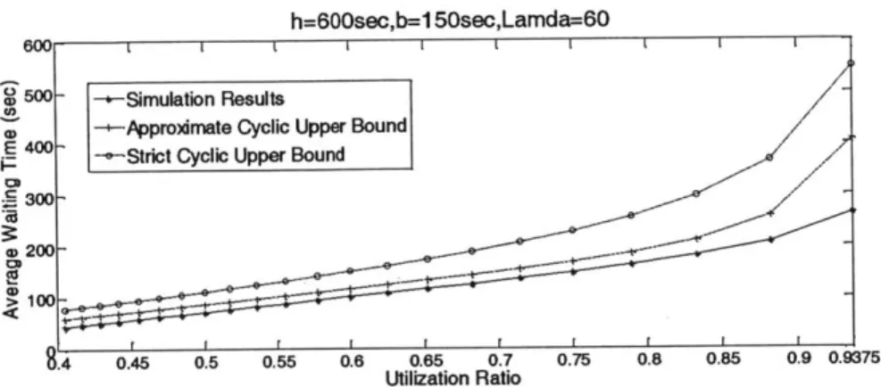
Figure 9: Simulation results and cyclic upper bounds of average waiting time when A = 60...51

Figure 10: Simulation results and cyclic upper bounds of average waiting time when A = 80. ... 51

Figure 11: Rectangular service region ... 53

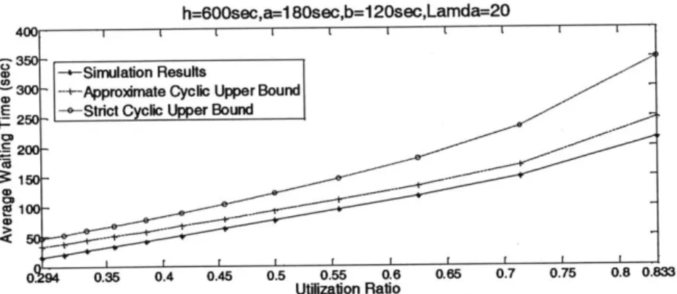
Figure 12: Simulation results and cyclic upper bounds when a = 180sec, b = 12Osec,A = 20 54 Figure 13: Four-sided diamond service region...61

Figure 14: Simulation results and cyclic upper bounds of diamond service region when b = 150sec,A = 20 ... 6 1 Figure 15: Rectangle service region with barrier inside ... 67

Figure 16: Simulation results and cyclic upper bounds, rectangle service region with barrier, w hen A = 2 0...68

Figure 17: Area division for the rectangle with barrier... 69

Figure 18: Greedy routing strategy for the General-Capacity, Multi-Vehicle LMP...79

Figure 19: Simulation and analytical results when c = 3 and A = 40...107

Figure 20: Simulation and analytical results when c = 3 and A = 80...107

Figure 21: Simulation and analytical results when c = 3 and A = 120 ... 107

Figure 22: Simulation and analytical results when c = 5 and A = 80...108

List of Tables

Table 1: Simulated and approximate middle leg expectation... 94

Table 2: Middle leg expectation approximation after regression correction... 95

Table 3: Simulated and approximate middle leg second moment... 96

Table 4: Middle leg second moment approximation after regression correction... 97

1. Problem Introduction, Description, Assumptions

and Overall

Approach

1.1 Introduction and Literature Survey

The Last Mile Problem (LMP) refers to the provision of travel service from home or workplace to the nearest public transportation node ("first mile") or vice versa ("last mile"). This public transportation node could be the nearest rapid transit rail station or a stop of a scheduled bus line. The unavailability of this type of service is one of the main deterrents to the use of public transport in urban areas, especially for certain demographic groups, such as schoolchildren, seniors and the disabled. Currently, the default solutions to the LMP are walking, taking a taxi, or driving a private vehicle.

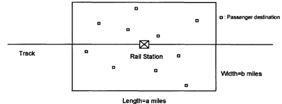
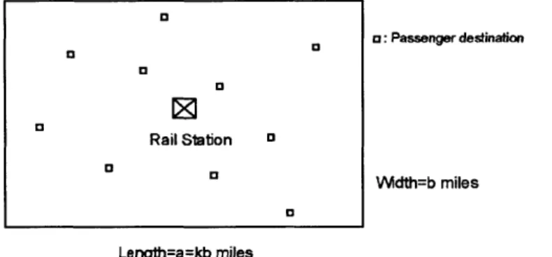
A conceptual Last Mile Transportation System (LMTS) is described schematically in

Figure 1, which shows an urban area surrounding a public-transit rail station, where trains arrive and discharge passengers. The passengers' final destinations (homes, offices and workplaces) are distributed in the area. A fleet of vehicles transports these passengers to their eventual destinations and empty vehicles return to the station to pick up waiting passengers or newly arriving ones. We describe the setting in more detail latter in Chapter 1.2.

o: Passenger destination

Trc _{Rail Station a}

Width=b miles

Length=a miles

Many issues must be addressed when designing and operating a LMTS. On the supply side, it is essential to deal with difficult questions concerning the stochastic aspects of the system. The demand side requires an understanding and estimation of the potential LMTS loads as a function of demographic characteristics, nature of trip, level of service, cost, etc.

The focus of this thesis is solely on the supply side: given a probabilistic description of demand, design a LMTS that operates under dynamic and stochastic conditions according to certain guidelines and satisfies a set of Level of Service (LOS) requirements. This implies specifying such system characteristics as vehicle fleet size, service frequency, dynamically varying vehicle schedules, vehicle dispatching strategies, vehicle routing strategies, monitoring and control of operations, etc.

Addressing these questions is difficult analytically, as the planning and management of a LMTS generally involves such complications as: stochastic travel times that may also change dynamically by time-of-day, according to traffic and weather conditions; batch arrivals of prospective passengers; partitioning of demands among vehicles; routing of the vehicles; queuing issues; and, obviously, numerous considerations conceming staffimg and economic sustainability. With the exception of staffmg and economic issues, we address most of these complications in this thesis in a static setting.

An extensive literature in this general area has generated various models for a number of application contexts related to the LMP with early papers dating back to the 1970s. We mention here only a few that are among the most influential in the field, as well as relevant to the approach we have adopted.

The Dynamic Traveling Repairman Problem (DTRP) was introduced in two papers

by Bertsimas and Van Ryzin. They consider the DTRP in the cases of a single-vehicle

"fleet" [1] and of multiple vehicles [2]. The Dynamic Pick-up and Delivery Problem (DPDP) was studied by Swihart and Papastavrou [3], who derived bounds on the performance of several DPDP variants for light and heavy traffic. The Car Pooling Problem (CPP), introduced by Baldacci, Maniezzo and Mingozzi [4] also has features similar to the LMP - or, more exactly, to the First Mile Problem. This paper presents

both exact and heuristic methods for solving the CPP based on integer programming formulations. Finally, a large number of papers have dealt with the Dial-a-Ride Problem (DARP) - see, e.g., Jaw, Odoni, Psarafis and Wilson [15]. A fine critical review of the DARP literature by Cordeau and Laporte [5] underlines, among other points, the fact that this body of work does not address well some of the queuing aspects of the subject systems - a deficiency that this thesis tries to remedy.

It should also be noted that similarities exist between the LMP and various queuing, dispatching, routing, and resource allocation problems arising in entirely different contexts such as the design of manufacturing systems, the operation of elevator banks, and the scheduling of school-bus systems.

The major difference between the LMP and the more "traditional" problems identified above is that, in the LMP, passengers arrive in (possibly large) batches, not singly. Moreover, the size of these batches is a random variable. Queuing systems with batch arrivals are notoriously difficult analytically. A further complication is that the "service times" of passengers are determined by the length (or the duration) of the routes traveled by the fleet of delivery vehicles. Thus, in designing a LMTS, it is necessary to consider simultaneously the problems of: allocating passengers among vehicles; routing the vehicles and estimating the lengths of the routes; and computing the queuing performance characteristics of the system.

The main body of this thsis is organized as follows. In latter Chapter 1, we describe in more detail the version of the LMP problem that we are studying and discuss the associated fundamental assumptions. It will be seen that the problem analyzed is quite generic and that by relaxing one or more of the assumptions, one can capture a broad range of interesting variations. Then we outlines the overall approach utilized to derive our results: we begin by deriving a set of queuing results by considering a fleet of vehicles with capacity for a single passenger (c = 1) and then extend the analysis by

allowing the vehicle capacity to be arbitrary and by incorporating the resulting travel time estimates into the queuing expressions derived for the c = 1 case. Chapter 2 presents our analysis and results for the single-capacity case. We derive three different approximate expressions for queuing performance as a function of the design parameters of the LMTS

and then identify, through a set of simulation experiments, the expression that performs best - and, in fact, approximates very well the observed waiting times. Chapter 3 first derives approximate analytical expressions for the travel times associated with fleets consisting of vehicles with a capacity of up to 20 passengers and then applies the queuing approximation derived in Chapter 2 to the multi-passenger capacity case. The results again compare well with those obtained from a simulation. The main part of Chapter 2 and 3 contain only outlines of the lengthy derivations of our results. A sequence of technical sections provides the details following the corresponding main part. Finally,

Chapter 4 contains a summary and concluding remarks.

1.2 Problem Description and Assumptions

We now describe in more detail the LMP scenario of Figure 1. The Last Mile Transportation System (LMTS) would operate as follows: Let STA be the transit rail station served by the LMTS and consider a passenger, PAX, who will board a train at station ORIGIN for the purpose of traveling to STA and will then board a LMTS vehicle for transport to her home. PAX will be required to provide advance notice to LMTS of her impending arrival at STA. The time interval between the advance notice and the actual arrival of PAX at STA will be of the order of several minutes (e.g., at least 5 or 10 minutes) to give the LMTS system sufficient time to plan the service of PAX. In practical terms, the advance notice could be generated by PAX in a number of alternative ways. For example, PAX could use a smart-phone when she arrives at ORIGIN or when she enters her train to STA; or, she could tap a smart card on a special-purpose screen, as she is entering ORIGIN or while aboard the train. The resulting message to the LMTS will include the expected time of arrival of PAX at STA (easy to predict, once the passenger is at the ORIGIN station or aboard a train) and her ultimate destination, e.g., her home address. (If the great majority of LMTS users will be subscribers whose home addresses will be pre-registered on a file, then the only information that PAX would have to provide will be an identification number.)

Once the information about PAX is received the LMTS will assign PAX to one of the vehicles of the LMTS fleet, plan the route of that vehicle so it includes a visit to the ultimate destination of PAX, estimate the departure time of the vehicle from STA, and notify PAX accordingly. PAX will receive a message (on her smart-phone or by tapping her card on a screen when she arrives at STA) that indicates the vehicle she has been assigned to and the planned departure time of the vehicle from STA (e.g., "please board Vehicle 123 which will depart from STA at 4:26 PM"). Once all the passengers assigned to a vehicle are on board, the vehicle will execute a delivery route, visiting the destination of each of the passengers and will then retum to STA to pick up the passengers for its next delivery tour.

The LMTS described above may be difficult to implement due to many practical issues and considerations. However, we have chosen to study it because it possesses the generic system features that we are most interested in: arrivals of passengers in "batches" (groups) at STA; "real-time" clustering of passengers for assignment to a fleet of vehicles; "real-time" routing of the vehicles to deliver the passengers on board; and fast computation of waiting times and other performance parameters so that, for example, passengers can be notified in a timely way of the departure time of the vehicle they have been assigned to/ informed of the expected departure times and intended use of the LMTS. Actual implementations would involve some simpler variants of the above features.

Given the service region geometry, passenger demand rates, the spatial distribution of the passenger destinations, and the number, capacity and travel speed of the LMTS vehicles, examples of performance metrics that we eventually wish to compute include: the average waiting time until boarding a delivery vehicle, the average riding time of passengers, the average waiting time until delivery, the minimum number of vehicles we need to reach stable operation, vehicle productivity and workload, and eventually (but not in this thesis) the general cost of operating the system and various service vs. cost

trade-offs.

We now identify briefly the specifics of the model considered. With reference to Figure 1, we make the following assumptions: (i) headways, h, between arrivals of trains

at the station (and discharges of passengers) are constant; (ii) passengers are discharged in batches after each train's arrival; (iii) the batch size is a general random variable, , with known expected value, E(f) = A, and variance, Var(f) = of; (iv) all passengers

arriving in a single batch request service essentially simultaneously; (v) given the size of any particular batch, ( = f, the destinations of the (o passengers in the batch are distributed identically, uniformly and independently in a service region; (vi) the service region is convex and compact with known dimensions; (vii) the delivery fleet (or pick-up fleet, in the case of "First Mile" service) consists of m vehicles, each with integer capacity, c.

We believe that (i) - (vii) are adequately general assumptions for approximating, to a first order, the characteristics of many potential variations of LMTS. Note that our model includes the most difficult, from the analytical point of view, features that one might encounter in an LMTS: batch arrivals, stochastic demand, stochastic service times, and the presence of queuing phenomena interfaced with routing problems.

To ensure that the mathematical expressions presented in Chapter 2 and 3 below are adequately concise, we have also used the following three simplifying assumptions: (viii) the service area, where the destinations of the passengers are located, is a b x b square, with the train station, STA, located at the square's center; (ix) the travel medium is continuous, homogeneous, and planar; and (x) the travel speed is constant throughout the service region and equal to 1. We have studied a number of variants of assumptions (viii) and (ix), such as cases in which the region is not a square, or the travel metric is Euclidean or rectangular ("right-angle) or contains discontinuities (e.g., barriers to travel), and shown that such mild changes in the assumptions pose no particular challenges.

1.3 Description of Overall Approach

Chapter 2 and 3 of the thesis describe in detail our analysis and results. In this Chapter we provide a brief description of the overall approach we have followed to provide perspective for these detailed Chapters. We have adopted a perspective under

which the LMTS is regarded as a spatially distributed queuing system in which the demands are as described before (batch arrivals of passengers with a constant headway between the arrivals of successive batches). In line, with typical queuing terminology, we shall refer henceforth to passengers as "customers" of the spatially distributed queuing system. The m parallel servers (the vehicle fleet) serve customers in groups of c or smaller, where c is the capacity of each vehicle. The service time for each group is equal to the travel time associated with a vehicle tour that begins at the station/depot, visits each of the c (or fewer) customer destinations and returns to the station/depot to pick up a new group.

o: Passenger destination

Track

-Width=b miles

Length=a miles

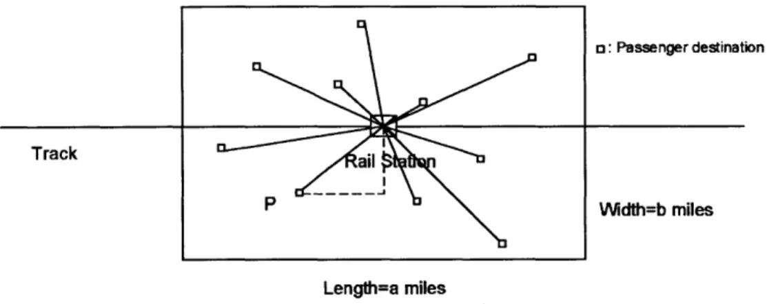
Figure 2: Customer destinations and vehicles routes of the Unit-Capacity, Multi-Vehicle LMP

Because queuing systems with batch arrivals (like the arrivals of passengers at STA) are notoriously difficult to analyze, we resort to a two-step approach. In Step 1, we assume that c = 1, i.e., that the delivery vehicles have unit capacity. Thus, in this case, service times consist simply of the duration of a round-trip between STA and one passenger's destination (see Figure 2), with the destination being randomly and uniformly distributed within the service area per our assumption (v) in Chapter 1. In this way we obtain a D /G/m/oo system in queuing theory notation, where: D indicates batch arrivals at constant ("Deterministic") intervals with the number of arriving passengers in each batch described by random variable (; G denotes the fact that the distribution of service times (i.e., the duration of the round trips between STA and customer destinations)

is "general"; and m and o indicate, respectively, the number of service vehicles and the fact that no a priori limit is placed on the number of customers waiting for pickup at STA.

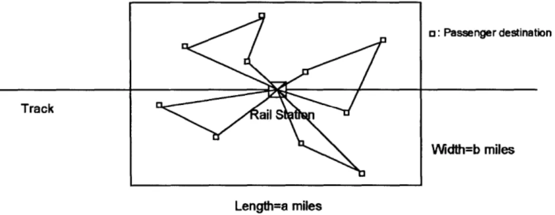
As no closed-form expressions are available for the fundamental quantities the performance of a Df/G/m/oo system, we then attempt to obtain expressions that would help us estimate performance by studying similar queuing systems, which are simpler to analyze mathematically. In this way, and through a series of simplifications, we derive one lower bound and two upper bounds for the mean waiting time associated with Df/G/m/oo queues. We then carry out an extensive series of simple simulation experiments and conclude that one of these three approximations (an upper bound) provides very good estimates of the performance of the system under a broad range of system design parameters. We therefore adopt this approximate expression for studying the general vehicle capacity case in which c can take on any (usually small) integer value. Step 2 examines this general case, in which service times are equal to the duration of delivery tours consisting of c(> 1) or fewer delivery stops, as shown in Figure 3. To

1: Passenger destination

Track _{all S}

Width=b miles

Length=a miles

Figure 3: Vehicle routes of the General-Capacity, Multi-Vehicle LMP

apply to the general capacity case the queuing expressions that were derived in Step 1, we need to compute in Step 2, the approximate length and the variance of the length of the vehicle tours shown in Figure 3. We accomplish this by using arguments from geometrical probability and from the literature on the Traveling Salesman Problem. We

obtain several such approximate expressions in this way and compare them with the results of another series of simple simulation experiments to select the expressions that fit best the observed expected values and variances of the vehicle tour lengths. We then use these expressions, along with the queuing-based approximation derived in Step 1, to complete the process of estimating the performance of the LMTS for the general case of arbitrary fleet size and arbitrary vehicle capacity.

The main part of Chapter 2 and 3 provide only an outline of the (occasionally lengthy) derivations of the results contained therein. The detailed mathematics is after the outline and between dash line.

2. The Unit-Capacity, Multi-Vehicle LMP

In this Chapter we consider the analysis of the Unit-Capacity, Multi-Vehicle case, described in Chapter 1 as Step 1, in which c = 1, and m is an arbitrary positive integer.

As already indicated above (Figure 2), the length of the vehicle trips in this case is equal to two times the distance between the rail station and a customer's destination. For the purpose of keeping relatively simple the various expressions derived, and without loss of generality, we shall assume that travel in the rectangular region of interest [Assumption (viii) in Chapter 1] is according to the right-angle metric, with directions of travel parallel to the sides of the rectangle. A typical route, for serving a particular customer P is indicated through a dashed line in Figure 2. Because we have also postulated [Assumption (x)] constant and unit travel speeds, the expressions for travel times in the region are identical with those derived for travel distances.

The basic notation is summarized as follows:

h = the constant headway between arrivals of trains at the station STA (and discharges of customers);

( = a random variable denoting the number of LMTS customers ("batch size") discharged after the arrival of a train at STA - with the sizes of successive batches being mutually independent and with E({) = A, and Var( ) = a denoting, respectively, the

expected value and variance of

f;

S= a random variable denoting the service time of any random LMTS customer with

E(S) = s and variance Var(S);

Note that the successive service times by any given vehicle in the fleet are independent and identically distributed. The traffic load (or utilization ratio) is given by p = sA/mh. Note that m/s is the service rate of the LMTS, while A/h is the rate of customer arrivals per unit of time. Technical Section 2.T presents some background results that are useful in the analysis of the Unit-Capacity, Multi-Vehicle case.

2.T*: Background Results

1. Expectation and variance of composite random variables;

Given a sequence of independent random variables X (i = 1,2, ..., N) , where N is also a random variable and independent of all the X, let Y = ZN X.

It is known [6] that:

E(Y) = E(N)E(X) _(2.T.1)

Var(Y) = Var(N)E 2 (X) + E(N)Var(X) _(2.T.2)

where E(Y),E(N) and E(X) denote the expected values, and Var(Y), Var(N) and Var(X) denote the variances of Y, N and X, respectively.

2. Total expectation and total variance:

Given two random variables X and Y, it is known [6] that:

E(X) = E(E(XIY)) _(2.T.3)

Var(X) = E(Var(XIY)) + Var(E(XIY)) _(2.T.4)

3. Exact solution for average waiting time in a M/G/1/oo queue:

In a M/G/1/oo queue, using the same notations as in the main part, it is known [7] that:

p 1+C_

WM/G/1/co = -p 2 s (2.T.5)

4. Bound for the average waiting time in a GI/G/1/oo queue;

In a GI/G/1/oo queue, let 1/Aa and s be the expected inter-arrival time and service time, respectively, y = 1/s the service rate, f, a2 the variances of the inter-arrival time and

inter-arrival time and service time, respectively, and p = Aas = Aa/p the traffic load (system utilization ratio). There is no simple explicit expression for the average waiting time W. According to [7],

p2(1 + C) - 2p < WGI/G1/O : Aa(Ca + CD) 21_{a( P)}

- WG/G1/ (2.T.6)

The upper bound becomes asymptotically exact as p - 1.

5. Approximation for average waiting time in a GI/0G/1/o queue;

In a GI/G/1/oo queue, using a combination of queuing theoretic and numerical analysis, the following two-moment approximation for the average waiting time in queue per customer was obtained by Kramer and Langenbach-Belz [8]:

e[ 2(1 -p)( -ca)2 C2: 1

p (cl+c)J 23p(c +

c

WGI/G/1/o 1 pC2 s, where p(C2T.7)

_exp

C

The approximation is useful for practical purposes provided that the traffic load of the system is not small and Ca is not too large. In the LMP, we will choose the number of vehicles so as to make sure the system utilization ratio (traffic load) is not small. Additionally, the constant headway of successive batch arrival (see the problem definition in the main part) means that CJ = 0. Therefore, the approximation could work well for the LMP.

2.1A Lower Bound

We are particularly interested in the expected waiting time, W, of LMTS customers until they board one of the m vehicles to be transported to their eventual destination. Determining this expected waiting time, as a function of the LMTS design parameters is a critical step toward developing the means to design LMTS satisfying certain level-of-service requirements. We begin by obtaining a lower bound for W.

Since no exact analytical solution exists for the complicated D /G/m/oo queuing model, we consider a modified system in which, instead of having batch arrivals with average size E({) at constant intervals (headway = h), we have a single arrival of a customer every h/E({) units of time. This modification transforms the original Df/G/m/

co system into a D/G/m/oo queuing system. The latter is characterized by a shorter average waiting time, W, than the original Df/G/m/oo system since the arrivals of customers are deterministic and evenly distributed, while the total expected number of customers served by the two systems is the same. However, no exact analytical solution exists for the D/G/m/o model either. Therefore, we consider instead a D/G/i/oo model, which has identical customer inter-arrival times with the D/G/m/co model, while its

single server works m times faster than each of the servers of the m-server system. Following the "remaining work inequality" principle of multi-server queuing models in

[9] and applying the approximation of GI/G/1/oo given in [7] (see Technical section 2.2.T)

we can then obtain (Technical Section 2.1 .T) a lower bound as follows: E({)E(S)E(S 2) + hE(S2

) - 2hE2 (S) - mhE(S2) 2E(S)(mh - E(f)E(S))

when the size of customer arrival batches,{, is drawn from a General distribution and the customer service time, S, is also drawn from a General distribution.

For the special case (Technical Section 2.1.T2 and 2.1.T3) in which the size of customer arrival batches is a Poisson random variable with intensity A and the service region is a b x b square:

-7mbh + 7bh + 7b2 A W 12(mh-bA)

2.1.T1 *: Lower Bound of Unit-Capacity, Multi-Vehicle LMP in the general case

According to the "remaining work inequality" for multi-server queuing model in [9], for the D/G/m/oo model and the corresponding D/G/1/oo model, constructed in the way described in main part Chapter 2.1, we have the following inequality:

p(M - 1)(a + 1/p 2 )

For the D/G/1/oo model, the average service time is reduced to s = E(S)/m, the service rate y = mIE(S), the service time variance o = Var(S)/m2, the coefficient of variation C2 = (Var(S)/m 2)/(E 2

(S)/m 2

) = Var(S)/E2(S), and the queue utilization ratio p = E( )E(S)/mh.

According to [7]:

(E(f)E(S))

p21

c)

E2

({)E 2(S) + Var(S)E2({) - 2mhE({)E(S)

2mE({)(mh - E(f)E(S)) (2.1.T1.2)

For the D/G/m/oo model, the service rate p = 1/E(S) and the service time variance ao2 = Var(S). We then have:

E2({)E2(S)+ Var(S)E2({) - 2mhE()E(S) E(S)(m - 1)(Var(S)+ E2(S))

WD//m/ --- 2mE({)(mh - E({)E(S)) 2m

E2({)E2(S)+ Var(S)E2(f) - 2mhE({)E(S) (m - 1)E(S2)

2mE({)(mh - E(f)E(S)) 2mE(S)

E({)E(S)E(S2) + hE(S2

) - 2 hE2 (S) - mhE(S2

)

2E(S)(mh - E({)E(S)) (2.1.T1.3)

This is the strict lower bound for the average waiting time in the original Df/G/m/oo model.

Under heavy traffic [9],

E() Var(S)

W l a ( O + J2 h m2 Var(S)E({)

D/G//o 2(1 -p) E()E(S) 2m(mh -E(f)E(S))

mh

E(S2

)E({) - E2

(S)E({)

2m(mh - E(()E(S)) (2.1.T1.4)

WD/G/m/co E(S2)E({) - E2(S)E(f) (m - l)E(S2) 2m(mh - E({)E(S)) 2mE(S) mE(f)E(S)E(S2) +mhE(S2 ) - m2hE(S2 ) - E3 (S)E({) 2mE(S)(mh - E({)E(S)) (2.1.T1.5)

This is the strict lower bound for the average waiting time under heavy traffic in the original D /G/m/oo model.

2.1.T2*: Service time distribution in a rectangular service region

Assume a rectangular service region A with dimensions of a along the horizontal axis and b along the vertical axis and with a > b . We also assume a right-angle ("Manhattan") travel metric with the directions of travel parallel to the sides of the rectangle. The train station is located at the center of the rectangular area and it is also the origin of our system coordinates. The maximum travel distance required to deliver a customer to his/her final destination and return to the station is a + b, while the minimum travel distance is 0.

Since the customer destinations are uniformly and independently distributed within the area and vehicles travel with unit velocity, successive travel times along the X-axis are uniformly and independently distributed in [0, a] with probability density function fx(x)= 1/a, 0 5 x < a; similarly, travel times along the Y -axis are uniformly and independently distributed in [O,b] with probability density function fy(y) = 1/b,0 < y5b.

Therefore, the total travel time S = X + Y, is described by the following probability density function: 1 s, 0:5 s:5 b; As(s) = h , b:5 s

5

₁₂

b2 7b2

E(S) = b,Var(S) = -,E(S 2

)

6 6

In the analysis above, we ignored any time required for loading and unloading customers.

2.1.T3*: Lower Bound of the Unit-Capacity, Multi-Vehicle LMP for a Poison customer

batch size and a square service region

If the number of customers from each train is Poisson-distributed and the service time is

as the square service region case described in Technical Section 2.1.T2, we consider a modified system in which, instead of having batch Poisson arrivals at the rate of A at constant intervals (headway =h), we have a continuous Poisson arrival stream at the rate of AL = A/h per unit of time. Both the original and modified systems have the same overall average arrival rate of A customers every h time units.

Considering the corresponding single (but m times faster) server model, the average service time is reduced to s = E(S)/m = b/m, the service rate y = m/b, the service time variance ao2 = Var(S)/m2 = b2/6m 2, the coefficient of variation of the service time C.2 = ao/s 2 = 1/6, and the queue utilization ratio p = A,/(m/b) = bA/mh. Thus:

bA bA

p 1+C 2 _ jj 1+1/6 b 7 -mT b 7b

2_A

W/-p 2 bA 2 m_12 1-

m

h

For the M/G/m/oo model, the service rate y = 1/b , and the service time variance ej = Var(S)/m2 ₌ b2 /6. Thus: 7b2 A A(m-1)(e|+ ) 7b2_{A (m-1)( +b2)} WM/G/m/-o Z" m 12 r(mh - bA) 2m 12m(mh - bA) 2mb 7b2 A 7(m - 1)b 7b2 A - 7(m - 1)b(mh - bA) 12m(mh - bA) 12m 12m(mh - bA) 7b2 A - 7m2 bh + 7mbh + 7mb2 A -7b 2A -7mbh + 7bh + 7b2A 12m(mh - bA) 12(mh - bA)

This is the strict lower bound for the average waiting time in the original Df/G/m/oo model.

Note that the expression above is correct dimensionally, with the dimension (unit) of the expression is first power of time.

2.2 Two Upper Bounds

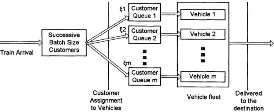
We next turn to obtaining an upper bound for W in the original Unit-Capacity, Multi-Vehicle D /G/m/oo model. To do this, we pre-assign customers to different vehicles and construct a corresponding single-server queuing model DN/G/1/oo for each vehicle, where N is the random variable indicating the number of customers from a single train assigned to the same vehicle.

With such an assignment policy, service inefficiencies exist since a customer is required to wait for his or her assigned vehicle, even when other vehicles may be available. Thus, the average waiting time in this case will be larger than the average waiting time in the original model and provides an upper bound. The customer flow is shown schematically in Figure 4 below.

Train Arrival

Customer Vehicle fleet Delivered

Assignment to the

to Vehicles destination

The DN/G/1/oo model is still difficult to work with. To obtain approximate expressions for W, we decompose the problem into two parts (Technical Section 2.2.T). First, the N customers in some batch who are assigned to the same vehicle are treated as a single "macro-customer" P. This reduces the DN/G/1/oo model to the more tractable D/G/1/oo model and allows us to obtain an upper bound for W, the expected waiting time until the first customer in P receives service. In a second step, we then compute the additional expected waiting time, W2, that the i-th customer in P suffers due to being

preceded for service by i-I other customers in P. Thus, the expected waiting time of a customer P is given by W = W1 + W2. In Technical Section 2.2.T we show that:

E(N)Var(S) + E 2(S)Var(N) 2(h - E(N)E(S))

W E (S)Var(N) + E(S)E 2 (N) - E(S)E(N)

2E(N)

Thus the upper bound we seek is: E(N)Var(S) + E 2

(S)Var(N) E(S)Var(N) + E(S)E2 (N) - E(S)E(N) (3)

2(h - E(N)E(S)) 2E(N)

The bound (3) is valid under general assumptions about the probability density functions of the batch size, (, and the service times, S. Moreover, (3) has been derived without considering how exactly customers are assigned to vehicles. We analyze next two different policies for customer assignment to vehicles. Each of these policies will provide different modified DNI/G/l/oo models with different E(N) and Var(N), leading to different expressions for W1 and W2, and, ultimately, different upper bounds for W.

2.2.T*: Upper bound for the average waiting time in the DNIG/1/00 queue model

We treat all the customers assigned simultaneously (in the same batch) to any given vehicle as a single "macro customer". If we only consider the macro customer, the DN/G/1/oo model can be reduced to a D/G/1/ce model. We denote the average waiting time of a macro customer in the D/G/l/oo model by Wm. WM is exactly equal to the

average waiting time of the first customer composited in the macro customer, which is denoted by W1, i.e., Wm = W1. The service time of the macro customer is T = E Si, where N is positive integer random variable indicating the number of real customers composing the macro customer. N depends on the assignment policy. S1,S2,,...,N are the service times of the real customers and they are mutually independent and identically distributed. Therefore,

N

E(T)= E(S) = E(N)E(S)

Var(T) = E(N)Var(S) + E2

(S)Var(N)

C2 _Var(T) - E (N)Var(S)+ E2 (S)Var(N)

E 2(T ) E 2(N )E2 (S)

a2= 0 (Due to constant batch or macro customer inter-arrival time) 1

E(T) E(N)E(S)

P h h

According to [9], the upper bound of W1, the average waiting time until the macro customer receive service, is:

1

=4 (aa + as2) - (0 + Var(T)) E(N)Var(S) + E (S)Var(N) 2

(1 - ) - 2(1 E(T) 2(h - E(N)E(S))

According to [8], an approximation of W1 is given by:

E(T) Var(T) 2

_1-W, ~ -) 2 _{-E(T) - exp -3 E(T) Var(T)}

h _{h E2(T) _}

2(h-E 3E(T)ar(T)

Var(T) 2(h - EcT))EcT)

2h-ET)3Var(T) (2.2.T.2)

When n = k, k > 1., the customer in the i th position will suffer the average waiting

time W! th = W1+ Q si, where s; is the average service time of the

j

With = W1 + (i - 1)E(S)

Let Wk denote the average waiting time of all the k customers, WiZt E =1[W + (i - 1)E(S)] (k - 1)E (S)

Wk = k k = W1 + 2 ,k 1

When n = 0, no customers served and WO = 0.

Let WDNG1/I denote the average waiting time of all customers in the DN /G1/cc

model. According to the Law of Total Expectation:

(k - 1)E(5) Zwk=P(n=k)Wkk r=oP(n=k)[WM+ 2 ]k WDNIG|1|w,- _{x=P(n=k)k -Z} 0P(n = k)k E-o P(n = k)Wmk 0 P(n = k)k _ (k- 1)E(S)k rk=oP(n= k) 2 k , 0 P(n = k)k

W,+ '=o P(n = k) (k - 1)k E (S) W,+E N 2) - E (N) E(S)

=1 =o P(n = k)k ₂ W 1 + E(N) 2

E(S)Var(N) + E(S)E2(N) - E(S)E(N)

2E(N) (2.2.T.3)

That is:

E(N)Var(S)+ E2(S)Var(N) . E(S)Var(N)+E(S)E2_{(N) - E(S)E(N)}

2(h - E(N)E(S)) 2E(N)

The first part

W

5

E(N)Var(S) + E 2 (S)Var(N)

2(h - E(N)E(S)) (2.2.T.5)

is the average waiting time until the first customer assigned to the vehicle in one batch receives service.

The second part = W, +

E(S)Var(N) + E(S)E2 _{(N) - E(S)E(N) (2.2.T.6)}

2E(N)

is the average waiting time due to the service time of customers served before in the same batch.

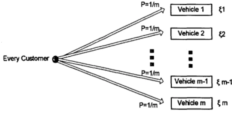
2.2.1 Randomized Assignment Policy

One possible policy is to assign all the customers randomly (with equal probability 1/m) and independently to the m different vehicles, with every vehicle serving individually the stream assigned to it. This is illustrated in Figure 5 below:

P=1/m _{Vehicle 1} (1 P=l/m Every Customer Vehicle m-I 1 m-1 P=ilm Vehicle m m Figure 5: Randomized assignment policy

The model corresponding to the randomized assignment policy led (Technical Section 2.2.1.Tl) to the following strict upper bound for the case of a General distribution of customer batch sizes and a general distribution of customer service times:

W mhE(S)E({2) - mhE(S)E(() + mE(S2

)E2

(f) - E2

(S)E3

(f) (4)

2m(mh - E(f)E(S))E({)

When the customer batch size is a Poisson random variable and the service region is a b x b square, the strict upper bound (4) becomes (Technical Section 2.2.1 .T 1):

7b2Am+ 6b)Amh - 6b2

12

An approximate upper bound for the case of Poisson customer batch size and a square service region can also be derived. This last bound was obtained (also in Technical Section 2.2.1 .T2) using an approximate expression for the average waiting time of the GI/G/1/o queuing model given in [8]:

7b2A 4(mh-bA)1 bA

W:< -exp- + - (6)

12(mh-bA)

[

2.2.1.T1*: Upper bound of the Unit-Capacity, Multi-Vehicle LMP under randomized assignment policy in the general case

One possible assignment policy is to apportion all the customers randomly, uniformly and independently among the m different servers, with each server then serving its own stream of customers independently of all the other servers. The model corresponding to this randomized assignment policy is DNi/G/1/oo , where N, is the random variable indicating the number of customers assigned to server i. N1, N2, .. , Nm are identically

distributed, so all DNi/G1/o models can be taken as the same DN/G/1/o model, although N1, N2, ..., N. are not necessarily independent. Assume ( is the random variable

indicating the total number of customers coming from one train. Given ( , we know N1-B({, 1/m), in which B(n, p) is Binomial distribution with total number n and

individual probability p. Thus:

E(N|() =

-{(mn-1) Var(Nf) = 2

E({) E(N) = E(E(Nk{)) =

-Var(N) = E(Var(N|{)) + Var(E(NI)) = E (f(m- 1) + Var

(

Therefore,

E(N)Var(S) + E 2(S)Var(N) E (S)Var(N) + E(S)E2 (N) - E(S)E(N)

WDNG/|/|

~

E(f) Var(S) + E2(S) E (f )(m - 1) + Var( ) 2 h -E()E(S)

E(S) E({)(m - 1) + Var({)+ E(S) (E() 2 E E()

+

~M2

-E(S)

M~

2 Ef

< mE(f)Var(S) + (m - 1)E({)E2(S) + E2_(S)Var({) 2m(mh - E(f)E(S)) E(S)(Var({) - E({) + E2 (f)) 2mE({) mE(f)E(S2) + E2 (S)(E({2) - E2

(f) - E(()) E(S)(E({2) - E({))

2m(mh - E({)E(S)) 2mE({)

mhE(S)E({2

) - mhE(S)E(() + mE(S2_)E2_{(f) - E}2_(S)E3_{( )}

2m(mh - E(f)E(S))E(() (2.2.1.T1.1)

This is the strict upper bound for the average waiting time under randomized assignment policy in the general case.

2.2.1.T2*: Upper bound of the Unit-Capacity, Multi-Vehicle LMP under

randomized assignment policy for a Poisson customer batch size and a square service region

If the number of customers from each train is Poisson-distributed and the service time is

as the square service region case described in Technical Section 2.1.T2. If we use the randomized assignment policy, all the customers are randomly and uniformly assigned to m different servers. It is well known that if we assign each customer independently to serverj with probability 1/m for all

j,

Var(f) = A E({2)= Var({) +E 2 () = A+A2 E(S) = b Var(S) =-E(S2) =Var(S) + E 2(S) E(N) =-7b2 6 Var(N)

=--CJ2= 0 (Due to constant batch or macro customer inter-arrival time)

CS2= Ct2 E(N)Var(S) + E 2 (S)Var(N!) = E2(N)E2(S) A b 2 2 -T + m 7m A2 b2 m7 s=E(T)=E(N)E(S)=-E(T) E(N)E(S) bA = it m

Thus, using the conclusion of Technical Section 2.2.T, we can obtain a strict upper bound for the average waiting time in the original D /G/m/oo model:

mhE(S)E(f2_{) - mhE(S)E({) + mE(S}2 )E2

(f) - E2

(S)E3

(f) ~72m(mh - E(+)E(S))E({)

mhb(A + A2) - mhbA + my A2 - b2 A3 7b2Am + 6bAmh - 6b 2A2

2m(mh - Ab)A 12m(mh - bA)

Similarly, we have the approximation (using the same notations as in Technical Section 2.2.T):

[2() 1 C-) p (C+C) 2(1 -p)(1 -C) 2 W, - 1 - p 2 exp _{3p(C2 + C2) I} bA 7m bA -- bA 2(1-)] 1bA 2 me3 bI 7m 1 3mh 6A 7b2A 4(mh -bA) 12(mh - bA) 7bm

E(S)E(N) Var(N) - E(N) E(S)

2 E(N) 2 7b2

exp

J

Both the approximate upper bound and the strict upper bound are dimensionally correct. The strict upper bound is larger than the approximate upper bound.

Under heavy traffic,

P-+ 1, mh - bA --+ 0, exp -(m - +1,

the difference between the approximate and strict bounds is reduced to zero.

Note, as well, that in the limit, the ratio of the strict upper bound for the average waiting time under randomized assignment to the lower bound for the average waiting time:

Upper Bound Lower Bound

7b2A + bA

12(mh - bA) +2m A(7bm+ 6hm - 6bA) 7Abm -7mbh+7bh+7b 2 A1 7m(h -hm+ bM) ~ 7mh' m 12(mh - bA) when p -> 1. WD NIG1|w' (2.2.1.T2.2)

A

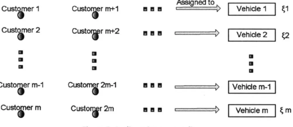
2.2.2 Cyclic Assignment Policy

Another possible policy is to assign customers in cyclic order to the vehicles: the first customer in the batch is assigned to Vehicle 1, the second to Vehicle 2, ... , the (m+1)-th to Vehicle 1 again, and so forth. No jockeying of customers, after being assigned to vehicles, is allowed. Figure 6 illustrates this policy, which requires assigning an "identification number" to each vehicle to distinguish among them.

Custo Ier m+1 Custorjr m+2 Assigned to E M I----K - Vehicle 11

s En

Figure 6: Cyclic assignment policy

|Vehicle

Vehicle m-i

Vehiclem ( m

The model corresponding to the cyclic assignment policy led (Technical Section 2.2.2.T1) to the following strict upper bound for the General distributions case:

W 4mE2({)E(S2

) - 4E2(S)E3

({) + 4mhE(S)E({2

) + m3hE(S) - 4m2_{hE(S)E({) (7)}

8m(mh - E(f)E(S))E()

For Poisson batch sizes and a square service region, the bound (7) becomes (Technical Section 2.2.2.T2):

14b2 2

m+ 12bA2mh - 12b2A3 + 12bAmh - 12bAm2h+ 3bm3h 24mA(mh - bA)

An approximate upper bound can also be obtained (Technical Section 2.2.2.T2) for the same case as (8): Cust ier 1 Cust er 2 U Custo er rn-1 Custo Wer m

(2m + 12)b2 A + 3 2M2 8(mh - b )A2

W 24m(mh - bA) (2m + 12)bA + 3bm]

4bA2 + 4bA + bm2 - 4bAm

+8AM (9)

A special case of (9) is also of interest in some applications. This is the case in which m/A is large, i.e., the number of vehicles in the fleet is large relative to the rate at which customers arrive. This can be the situation during off-peak periods or when the vehicle fleet consists of a large pool of bicycles available for shared use. In such cases (9) becomes (Technical Section 2.2.2.T3):

7b2 Am - 6b2₁2

4(mh - bA)

12m(mh - bA) 7bm - 6bA

The approximate upper bound (10) has the desirable property of becoming more accurate as p approaches 1. Since p = bA/mh, a large m/A means a large b/h when p approaches 1. This corresponds to situations in which the service region is large and/or the train

frequency is low.

2.2.2.Tl*: Upper bound of the Unit-Capacity, Multi-Vehicle LMP under cyclic assignment policy in the general case

This policy consists of assigning customers in cyclic order to the m servers. After each batch arrival, the 1st customer in the batch is assigned to the 1st server, the 2nd customer is assigned to the 2nd server, ... , the (m+1)-th customer is assigned to the 1st server again, and so forth. No jockeying of customers, after being assigned to vehicles, is allowed. We utilize different server orders for customers coming from different batches (trains).

There are totally m servers, with the name "Server 1", "Server 2",..., "Server m". Let Ni be the random variable indicating the number of customers assigned to "Server i" after the arrival of a particular train, with the assignment process upon arrival of each train being independent of the arrival process upon arrival of any other train.

After one train arrived, we order the m servers in sequence, the server receiving customers firstly is called "1st server", the server receiving customers secondly is called "2nd server", etc. Let X, be the random variable indicating the number of customers assigned to the "i th server" after the arrival of a particular train. Then,

SK+m-1r _ {+m-21i...'Xm....i 1 Xm =

f =X+X 2+---+Xm-1+Xm

The probability that Server i become the

j

The modified model can be considered as DNi/G/1/oo, which will provide an upper bound to the original D /G/1/oo model. N1, N2, ...,Nm are identically distributed, so all

DNi/G/1/oo models can be taken as the same DN/G/1/oo model, although N1, N2, ...,Nm are not necessarily independent. f is the random variable indicating the

total number of customers coming from one train. f = Km + R, where K =

[f/m],

X= _K+1, 1 i!R; IK, R +1: i m;

1

E(N|I(K, R))=-[E (X1|I(K, R)) + E(X2| (K, R)) +..+ E Xm|I(K, R))]

1 (+m-2Km+R ++m1 {

mL

m]

m]Xr

m~r

m

m

m