HAL Id: hal-02912135
https://hal.archives-ouvertes.fr/hal-02912135
Submitted on 5 Aug 2020
HAL is a multi-disciplinary open access
archive for the deposit and dissemination of sci-entific research documents, whether they are pub-lished or not. The documents may come from teaching and research institutions in France or
L’archive ouverte pluridisciplinaire HAL, est destinée au dépôt et à la diffusion de documents scientifiques de niveau recherche, publiés ou non, émanant des établissements d’enseignement et de recherche français ou étrangers, des laboratoires
Groundwater flow characterization of an ophiolitic
hard-rock aquifer from cross-borehole multi-level
hydraulic experiments
Gerard Lods, Delphine Roubinet, Jürg Matter, Richard Leprovost, Philippe
Gouze
To cite this version:
Gerard Lods, Delphine Roubinet, Jürg Matter, Richard Leprovost, Philippe Gouze. Groundwater flow characterization of an ophiolitic hard-rock aquifer from cross-borehole multi-level hydraulic ex-periments. Journal of Hydrology, Elsevier, 2020, 589, pp.125152. �10.1016/j.jhydrol.2020.125152�. �hal-02912135�
Preprint version Please cite as:
Lods G., D. Roubinet, J. M. Matter, R. Leprovost and P. Gouze (2020), Groundwater flow characterization of an ophiolitic hard-rock aquifer from cross-borehole multi-level hydraulic experiments, Journal of Hydrology, 125152, doi:10.1016/j.jhydrol.2020.125152
Groundwater flow characterization of an ophiolitic
hard-rock aquifer from cross-borehole multi-level
hydraulic experiments
G´erard Lodsa, Delphine Roubineta,∗, J¨urg M. Matterb, Richard Leprovosta, Philippe Gouzea, Oman Drilling Project Science Team
aGeosciences Montpellier, University of Montpellier, CNRS, Montpellier, France bOcean and Earth Science, National Oceanography Centre Southampton, University of
Southampton, United Kingdom
Abstract
Ophiolitic formations play a critical role in the groundwater resource of nu-merous countries and areas. Previous studies show that the structural hetero-geneities of these rocks, coming from the presence of both different litholog-ical units and multi-scale discontinuities, result in complex hydrogeologlitholog-ical features that are not well characterized yet. In particular, there is a need for understanding how these heterogeneities impact the hydrodynamic prop-erties of ophiolitic aquifers and the highly variable chemical composition of the water. To this end, we conduct various kinds of pumping experiments between two boreholes 15 m apart in the ophiolitic formation of the Batin (BA1) site in the wadi Tayin massif of the Sultanate of Oman. Cross-borehole open pumping experiments, as well as multi-level pumping and monitoring hydraulic tests, are performed in conductive zones that were identified from temperature and flowmeter data, but also in low-permeability zones requiring
to manage very low pumping flow rates. The collected data are interpreted with a model implementing non-integral flow dimension, leakage and time-dependent pumping flow rates. The considered modeling concepts and the estimated hydrogeological properties show that the multi-directional struc-tural heterogeneities of ophiolitic aquifers are key features that must be con-sidered in future hydrogeological models because they drive the hydraulic responses of these systems.
Keywords: Ophiolitic aquifer, Cross-borehole hydraulic test, Multi-level packer pumping experiment, Heterogeneous hydrosystems, Hydraulic property estimation, Variable flow-rate model
1. Introduction
1
Ophiolitic rocks are fragments of oceanic crust and upper mantle which
2
are widespread on the surface of continents along tectonic suture zones (e.g.,
3
Abbate et al., 1985; Boronina et al., 2005; Maury and Balaji, 2014; Segadelli
4
et al., 2017b; Vacquand et al., 2018; Jeanpert et al., 2019). These rocks
ex-5
tend from the Alps to the Himalayas through, for instance, Cyprus, Syria
6
and Oman, and are also present in various countries such as Cuba, USA,
7
Papua-New Guinea, New Caledonia and Newfoundland (Abbate et al., 1985).
8
Ophiolites are important groundwater resources in some areas (e.g., within
9
the northern Apennines (Segadelli et al., 2017b) and in Cyprus (Boronina
10
et al., 2005)). In Oman, ophiolite water was a key resource for the
popu-11
lation that started in 3000 BC. Nowadays, the main fresh water supply in
12
the towns bordering the Oman gulf including Muscat comes from sea
wa-13
ter desalinisation, but ophiolites still provide the only source of water for
agriculture (including dates growing, which is often the main income for
vil-15
lagers) in several inland areas where people built underground galleries called
16
Aflaj (plural of Falaj) for irrigation since 5000 years. Villages developed close
17
to the (often intermittent) rivers (wadis) that form from the ophiolite
wa-18
ter sources often occurring at the peridotite - gabbro interface, the former
19
forming the low permeability reservoir while the latter, fractured and often
20
altered, draining the ophiolite massif water toward sources (Dewandel et al.,
21
2004). In a general manner, ophiolites may impact strongly the chemical
22
composition of the water (e.g., in western Serbia (Nikic et al., 2013) and
23
Oman (Paukert-Vankeuren et al., 2019)) because of the high reactivity of
24
the rock-forming minerals which makes some water sources unsuitable for
25
human use. Ophiolites are composed of rocks such as basalt, dolerite,
gab-26
bro and peridotite, implying that they are characterized by the coexistence
27
of different lithological units, which can be fractured at many scales due
28
to cooling and (multiple) chemical alteration mechanisms. The presence of
29
structural discontinuities that control the permeability of these systems
re-30
sults in some similarities with the well-known and widely-studied fractured
31
granitic rock aquifers. However, these similarities in terms of fracturation do
32
not result in similar overall systems since the submarine conditions of
for-33
mation of ophiolitic rocks and weathering after exumation lead to complex
34
hydrogeological properties that are not well characterized yet (e.g.,
Boron-35
ina et al., 2003; Dewandel et al., 2005; Jeanpert et al., 2019). For instance,
36
at meter to tens of meters scales, far from faults, hydraulic discontinuities
37
in peridotites are often zones concentrating high density of fissures whereas
38
granite systems are usually homogeneous, poorly-permeable matrix hosting
pluri-meter scale, often sparsely distributed, discrete fractures.
40
The few studies conducted on ophiolitic aquifers show that the structural
41
heterogeneities of these systems, resulting from the presence of both different
42
lithological units and multi-scale hydraulic discontinuities (from fissure zones
43
to kilometer-scale faults), control their inherent behavior under ambient
con-44
ditions and their responses to forced conditions. As a result, the
hydrogeo-45
logical models that are built to understand and reproduce the hydrodynamic
46
of these aquifers are based on the coexistence of various recharge and
trans-47
missivity zones, which hydraulic properties depend on the lithological units
48
and discontinuities that are associated with the zones (e.g., Boronina et al.,
49
2003; Dewandel et al., 2005; Segadelli et al., 2017a). These properties are
50
estimated from different characterization techniques, including hydrograph
51
analysis, mercury porosity and hydraulic conductivity laboratory
measure-52
ments, as well as pumping tests (e.g., Boronina et al., 2003; Dewandel et al.,
53
2005; Jeanpert et al., 2019).
54
The large variety of existing techniques and possible configurations that
55
are associated with pumping experiments makes it a very useful tool for
56
characterizing the subsurface hydraulic properties. Conducting these
ex-57
periments in open boreholes, or using single or dual packers that are moved
58
along the boreholes, provide vertically-integrated or vertically-distributed
hy-59
draulic properties, respectively. The resulting changes in pressure are
mon-60
itored in either the pumped well (i.e., single-borehole experiments) or
ob-61
servation wells (i.e., cross-borehole experiments), which impacts the spatial
62
extent and meaning of the estimated properties (e.g., Bear, 1979; Le Borgne
63
et al., 2007; Day-Lewis et al., 2011). That being said, the quality of these
estimates depends on the models that are used to interpret the collected
65
hydraulic data. The line-source analytical solutions (e.g., Theis solution),
66
which are widely used because they are easy to implement, are well suited
67
for interpreting the intermediate and late-time responses that are collected
68
while applying steady pumping flow rates. However, the assumption of a
69
negligible effect of the pumped borehole storage might be critical when
in-70
terpreting early-time data related to transient pumping flow rates. Using
71
more sophisticated solutions, which take into account the wellbore storage
72
effect, the flow dimension related to the structural heterogeneities, and the
73
occurrence of leakage effects, leads to better estimates of the hydraulic
prop-74
erties of the studied systems, in particular when focusing on heterogeneous
75
systems and time-dependent pumping flow rates (e.g., Lods and Gouze, 2004;
76
Cihan et al., 2011; Yeh and Chang, 2013).
77
In the context of ophiolitic aquifers, only a few studies considered
pump-78
ing tests for characterizing these hydrosystems (e.g., Boronina et al., 2003;
79
Dewandel et al., 2005; Jeanpert et al., 2019). For the Kouris catchment in
80
Cyprus and the Koniambo massif in New Caledonia, hydraulic
conductiv-81
ity estimates were obtained from single-borehole pumping experiments and
82
packer tests, respectively, that are interpreted with simple analytical
solu-83
tions (Boronina et al., 2003; Jeanpert et al., 2019). For the ophiolite
hard-84
rock aquifers in Oman, the interpretation of open cross-borehole pumping
85
experiments with a dual-porosity (or dual-permeability) model led to
esti-86
mate the hydraulic conductivity and storage coefficients at various locations
87
(Dewandel et al., 2005). These studies emphasized that the efforts for
char-88
acterizing ophiolitic aquifers with pumping experiments need to be pushed
further by focusing on (i) conducting multi-level pumping experiments (i.e.,
90
packer tests) in order to obtain vertically-distributed estimates of the
hy-91
draulic properties, (ii) using sophisticated models for improving the quality
92
of the estimated properties, (iii) combining the complementary information
93
provided by open borehole experiments and packer tests where the packers
94
can be used for multi-level pumping and multi-level pressure monitoring, and
95
(iv) developing pumping techniques and specific equipment that are adapted
96
to low permeability zones with localized highly-permeable structures.
97
In this work, we address these challenges by conducting and analyzing
98
several kinds of pumping experiments in the ophiolitic Batin East site in
99
the Wadi Tayin massif of the Sultanate of Oman. To this end, we start by
100
analyzing open borehole pumping experiments that were conducted in two
101
boreholes (positioned 15 m apart), and we show that the considered systems
102
cannot be characterized with vertically-integrated hydraulic properties. In
103
order to infer vertically-distributed properties, we then consider multi-level
104
pumping experiments, as well as multi-level cross-borehole pressure
monitor-105
ing, with intervals defined from temperature and flowmeter data. In light
106
of direct geological observations and indirect data analysis, we consider
non-107
integral flow dimension models with vertical leakage that are used in the
108
context of time-dependent pumping flow rates. The corresponding results
109
show the complexity of the studied system for which both the lithological
110
units and discontinuities impact the estimated hydraulic properties in
dif-111
ferent proportions depending on the considered layer. In this work, we also
112
address the issue of pumping tests in poorly-permeable zones by
present-113
ing material, experimental methods and interpretation procedures especially
adapted to this challenge.
115
The site and methods are described in Section 2, the pumping experiments
116
and their interpretation are discussed in Section 3, and the results and general
117
conclusions are presented in Sections 4 and 5.
118
2. Site and methods
119
2.1. Site description
120
The International Continental Scientific Drilling Program (ICDP) Oman
121
Drilling Project (OmanDP) established a multi-borehole observatory in Wadi
122
Lawayni in the Wadi Tayin massif of the Samail ophiolite in 2018 to study
123
ongoing weathering processes, the associated hydrogeological system, and
124
the subsurface microbiome. Wadi Tayin massif is one of the largest and
125
most intact massifs within the Samail ophiolite. The observatory lies within
126
the mantle peridotite section, approximately 3 km north of the crust-mantle
127
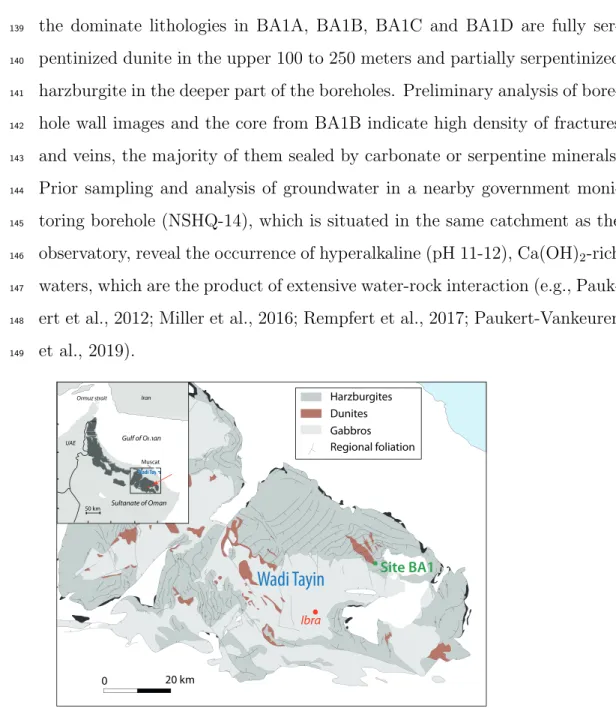
transition zone (MTZ) in the south-eastern part of the massif (Figure 1). The
128
MTZ and surrounding crustal gabbroic and mantle rocks are displaced by
sev-129
eral kilometres along a set of NNW trending, strike-slip faults (e.g., Nicolas
130
et al., 2000). A prominent NNW trending fault system, with unknown sense
131
of displacement, cuts across Wadi Lawayni and the multi-borehole
observa-132
tory (Figure 1). The observatory consists of a multi-borehole array of drill
133
sites, including BA1, BA2A, BA3A and BA4A. Site BA1, which is the target
134
site for this study, includes one fully cored, 400 meter deep hole (BA1B) and
135
three rotary-drilled, 400 meter deep, 6-inch diameter holes (BA1A, BA1C
136
and BA1D) (Figure 2). Borehole BA1C collapsed at 60 meters depth shortly
137
after drilling and was abandoned. Based on core and drill cutting analysis,
the dominate lithologies in BA1A, BA1B, BA1C and BA1D are fully
ser-139
pentinized dunite in the upper 100 to 250 meters and partially serpentinized
140
harzburgite in the deeper part of the boreholes. Preliminary analysis of
bore-141
hole wall images and the core from BA1B indicate high density of fractures
142
and veins, the majority of them sealed by carbonate or serpentine minerals.
143
Prior sampling and analysis of groundwater in a nearby government
moni-144
toring borehole (NSHQ-14), which is situated in the same catchment as the
145
observatory, reveal the occurrence of hyperalkaline (pH 11-12), Ca(OH)2-rich
146
waters, which are the product of extensive water-rock interaction (e.g.,
Pauk-147
ert et al., 2012; Miller et al., 2016; Rempfert et al., 2017; Paukert-Vankeuren
148 et al., 2019). 149 0 20 km Muscat Gulf of Oman Iran UAE Sultanate of Oman Ormuz strait 50 km
Wadi Tayin
Harzburgites Dunites Gabbros Regional foliation Ibra Site BA1Wadi Tayin Ibra
Figure 1: Map of the Wadi Tayin massif with the location of Site BA1 (modified after No¨el et al. (2018), redrawn after Nicolas et al. (2000)). In inset, location of the Wadi Tayin massif in the Semail Ophiolite (North of Sultanate of Oman; redrawn after Einaudi et al. (2000)).
Figure 2: (a) Local geological map of Wadi Lawayni, Samail ophiolite (redrawn after Bailey (1981)). (b) Location of boreholes forming the BA1 multi-borehole observatory site.
2.2. Material and method
150
Figure 3 displays the schematic representation of the downhole part of
151
the pumping system. It is installed from the surface using a tripod equipped
152
with an electric chain hoist as a succession of individual parts of maximum
153
3 m length that are assembled at the surface. From the bottom to the top,
154
the dual-packer system includes:
155
- the lower pressure port (P1) that measures the pressure below the lower
156
packer;
157
- the lower packer. The two packers are 1 m long and can be inflated
in-158
dividually so that one can perform single-packer or dual-packer pumping
test depending on the objectives;
160
- the pumping interval that can be set to a length ranging from 1 to 30 m;
161
- the intermediary pressure port (P2) that measures the pressure in the
mea-162
surement interval;
163
- the upper packer;
164
- the upper pressure port (P3) that measures the pressure above the upper
165
packer. P3/ρg measures the water column length above the upper packer,
166
ρ and g being the fluid density and gravitational acceleration, respectively;
167
- the shut-in valve. When the packers are inflated, the valve is closed due to
168
the weight of all the equipment (pump and pipes) above it. It is opened
169
by pulling the pipe assemblage from the surface with the crane;
170
- a stack of PVC pipe of length determined in order to position the pump
171
according to the depth of the upper packer and of the water table while
172
keeping a distance of 10 to 150 m below the water test static level (WTSL);
173
- the pump (Grundfos SQE 1-140)
174
The downhole system displayed in Figure 3 is installed below the required
175
length of screwed PVC pipes of internal diameter 48 mm. The system is
176
linked to the surface by the electrical wire required for powering the downhole
177
pump as well as the data wire used to transmit the multiplexed data from
178
the pressure sensors (that also measure temperature) and the gas hoses for
179
inflating/deflating the packers that are included into a single cable. The
180
data including the pressure at the three measurement levels P1, P2 and P3
181
are recorded at the surface together with the two packer pressures and the
182
water flow rate measured by a flowmeter installed in-line at the well-head.
2.3. Experiments and models
184
Three kinds of pumping experiments are considered for characterizing the
185
BA1 site presented in Section 2.1 with the material and method described in
186
Section 2.2. (i) Cross-borehole pumping tests are conducted with the
pres-187
sure being monitored in both (open) observation and pumped boreholes
(Sec-188
tion 3.1). These experiments are denoted Exp1A and Exp1D when pumping
189
in boreholes BA1A and BA1D, respectively. (ii) Multi-level pumping tests
190
are conducted by using packers in order to isolate and pump in specific
in-191
tervals of the pumped borehole while the pressure is monitored between the
192
packers (P2), above the upper packer (P3), and below the lower packer (P1),
193
as well as in the (open) observation borehole. The intervals considered for
194
these experiments were determined from the analysis of profiles of
tempera-195
ture and flowmeter data, the latter profile being collected under ambient and
196
forced hydraulic conditions. This data are presented in Appendix A with
197
the pressures P1 and P3 that are monitored below and above the packers,
198
whereas pressure P2 is analyzed in Section 3.2. The corresponding
experi-199
ments are denoted Exp2A i1A and Exp2A i2A when pumping is performed
200
in the intervals i1A (41-65 m) and i2A (108-132 m) of borehole BA1A, and
201
Exp2D i1D and Exp2D i2D when pumping is performed in the intervals i1D
202
(45-75 m) and i2D (102-132 m) of borehole BA1D. For both boreholes, we
203
also consider the zone below 132 m (i.e., 133-400 m), denoted i3A and i3D,
204
in order to characterize the low-conductivity zone that is located at the
bot-205
tom of the wells. The corresponding experiments are denoted Exp2A i3A
206
and Exp2D i3D when pumping in borehole BA1A and BA1D, respectively.
207
(iii) Finally, a cross-borehole multi-level-monitoring pumping experiment,
denoted Exp3D (Section 3.3), was conducted by using the packer system in
209
borehole BA1A while pumping in borehole BA1D with a Grundfos SQ2-85
210
pump. This test consisted in monitoring the pressure at several isolated
po-211
sitions in the observation borehole while the pressure is also monitored in
212
the (open) pumped borehole.
213
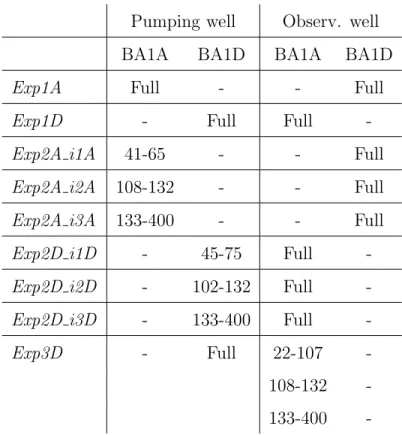
Table 1 summarizes the pumping and observation parameters of the
ex-214
periments by indicating in which borehole and at which position the pumping
215
and monitoring are done. ’Full’ corresponds to open boreholes, whereas the
216
numbers indicate the distances in meter from the surface to the top and
217
bottom positions of the packers that are used to consider isolated intervals.
218
During all these experiments, the pressure was also monitored in borehole
219
BA1B (120 m NNW of BA1A and BA1D), in which no response was recorded.
220
This is likely due to the low permeability of the corresponding zone as shown
221
by the log data and core analysis of this borehole (not shown).
222
From a modeling point of view, the fractured nature of ophiolitic aquifers
223
leads to consider both dual-permeability and non-integral flow dimension
224
models, the former modeling concept being used in some previous studies
225
(Dewandel et al., 2005). Here, we focus on the latter conceptual models
be-226
cause of the following reasons: (i) Direct surface observations at the scale
227
of the test site showed numerous heterogeneously distributed centimeter to
228
decimeter-scale fractures but no large-scale hydraulic discontinuities such as
229
fractures that would have suggested the presence of two interconnected
sys-230
tems of distinctly different hydraulic properties, and as such should have
231
justified the use of dual-permeability models. (ii) The responses recorded
232
above and below the isolated intervals during packer tests with the pressures
Pumping well Observ. well
BA1A BA1D BA1A BA1D
Exp1A Full - - Full
Exp1D - Full Full
-Exp2A i1A 41-65 - - Full
Exp2A i2A 108-132 - - Full
Exp2A i3A 133-400 - - Full
Exp2D i1D - 45-75 Full
-Exp2D i2D - 102-132 Full
-Exp2D i3D - 133-400 Full
-Exp3D - Full 22-107
-108-132
-133-400
-Table 1: Setup at the pumping and observation boreholes for the set of hydraulic tests
P1 and P3 that are reported in Appendix A, show the presence of vertical
234
connections that can be modeled as vertical leakages in non-integral flow
di-235
mension models (Hamm and Bidaux, 1994). (iii) The results obtained in
Sec-236
tion 3 with non-integral flow dimension models are well in agreement with the
237
data and produce realistic estimations of the parameters and properties, thus
238
confirming that the use of more complex models (such as dual-permeability
239
models) is not necessary for the considered data. Dual-permeability models
240
involve more parameters and as such more degrees of liberty that generally
241
require making assumptions or using external data such as geophysical or
242
geological data. In the absence of such data that would have dictated using
dual-permeability models, the most parameter-parsimonious model must be
244
considered as the most probable model providing a fit to the data.
245
In order to interpret the data collected during these experiments, we
246
implemented a solution for transient radial flow in leaky aquifers with
time-247
dependent pumping flow rates using a fractal formalism. This
representa-248
tion is adapted to model hierarchical multi-scale fractured aquifers where
249
the characteristic length of the heterogeneity is smaller than the volume
in-250
vestigated by the pumping test (Lods and Gouze, 2008). We consider the
251
solution that is presented in Appendix B, which corresponds to an existing
252
solution for transient radial flow in a fractal fractured aquifer with leakance
253
that is extended to time-dependent pumping flow rates and non-linear skin
254
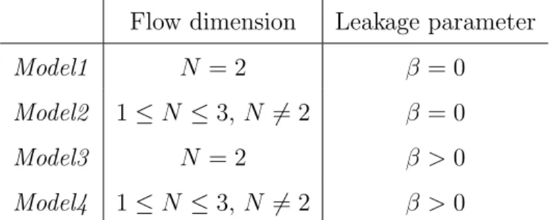
effects. From this solution, we derived four specific models corresponding
255
to (i) cylindrical flow without leakage (Model1 ), (ii) generalized radial flow
256
without leakage (Model2 ), (iii) cylindrical flow with leakage (Model3 ), and
257
(iv) generalized radial flow with leakage (Model4 ). The parameters that
258
distinguish these models from each other are summarized in Table 2. The
259
derivation of the models, the associated assumptions, and their use for
in-260
terpreting the data are given in Appendix C. The modeling strategy consists
261
in determining the model that best reproduces the values collected in both
262
the pumping and observation boreholes. When a common model cannot be
263
found, different models and parameters are considered for each borehole. We
264
select the best-fitting model by considering the quality of the overlap between
265
the curves of the simulated and collected data, as well as the physical meaning
266
of the estimated properties. For each experiment, the estimated parameters
267
of the models are presented in tables in which the parameters corresponding
to the selected best-fitting model are written in bold characters.
269
Finally, in order to have an independent estimate of the standard
trans-270
missivity T (Model1 ), the transmissivity value estimated by interpreting the
271
end of the recovery with Theis’ method (Kruseman and de Ridder, 1990)
272
is also provided. Since our models are based on unit-thickness aquifer
rep-273
resentations for Model1 (as explained in Appendix C), the estimated
hy-274
draulic conductivity values of Model1 are equivalent to transmissivity values
275
and will be directly compared to the transmissivity estimated with Theis’
276
method. The quality of the best-fitting models is also tested by estimating
277
the drawdown in borehole BA1B, for which, as mentioned before, no response
278
is observed during the pumping tests. The simulated values range from 0 to
279
36.07 cm, showing in the latter case the impact of heterogeneities in hydraulic
280
properties between the boreholes.
281
Flow dimension Leakage parameter
Model1 N = 2 β = 0
Model2 1 ≤ N ≤ 3, N 6= 2 β = 0
Model3 N = 2 β > 0
Model4 1 ≤ N ≤ 3, N 6= 2 β > 0
Table 2: Range of variations of the flow dimension (N ) and leakage parameter (β) for the four models considered for data interpretation. β = 1/B2 with B the leakage factor in Appendix B.
3. Experimental data and interpretation
282
3.1. Cross-borehole pumping tests
283
3.1.1. Pumping test in borehole BA1A
284
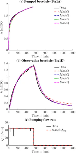
Figure 4 displays the data collected during the pumping experiment
285
Exp1A in the pumped and observation boreholes (black curve in Figures 4a
286
and b, respectively). In these figures, h is the difference in hydraulic head,
287
expressed in meter of water, between the beginning of the experiment (t = 0)
288
and time t. For technical reasons, h was not monitored in the pumped well
289
during the recovery period (Figure 4a). Figure 4c shows the pumping flow
290
rate monitored during the experiment (black curve), which was applied for
291
551 minutes with an average value of 44.9 L/min, and the flow rate
mod-292
eled with an exponential model (red dashed curve). The exponential model
293
is required for interpreting some of the experiments for which the flow rate
294
decreases noticeably. For this pumping test, the flow rate could have been
295
considered rightly as constant, but we applied the exponential model for
mat-296
ter of consistency. For this pumping test no common model reproducing the
297
data collected in both the pumped and observation boreholes could be found.
298
The models and parameters evaluated for each of the boreholes are given in
299
Table 3. Note that in this table, and in the rest of the manuscript, the values
300
of the skin factor (σw) and aquifer specific storage (Ss) that are estimated
301
from the pumped-borehole data are not shown because of their poor
relia-302
bility (Kruseman and de Ridder, 1990). However the variations of the skin
303
factor estimated from the pumped-borehole data are presented graphically
304
because their irregular variations reveal clogging/unclogging phenomena.
305
Concerning the data collected in the pumped borehole, Model1 and Model2
provide an acceptable fit, which could not be improved with the leakage
prop-307
erties that are considered in Model3 and Model4 (Figure 4a). For Model1, it
308
is important to emphasize that additional simulations (not shown)
demon-309
strate that σw remains negative for Ss< 1 m−1, which indicates the presence
310
of open fractures that intersect the well (Ahmed and Meehan, 2011). The
311
presence of channelized flow in a fracture network is also indicated by the
312
flow dimension smaller than 2 for Model2 (Le Borgne et al., 2004; Audouin
313
et al., 2008; Verbovˇsek, 2009). From the results presented in Figure 4a and
314
Table 3, this model is considered as the best-fitting model for the data
col-315
lected in the pumped borehole because it is the simplest model providing the
316
best fit to the data with the most realistic estimated parameters.
317
Different results are observed for the data collected in the observation
318
borehole. The transmissivity value estimated with Model1 is consistent with
319
that of the standard Theis’ method, which is equal to 1.27 × 10⁻⁴ m2/s. This
320
being said, Model2, Model3 and Model4 equally improve the fit between the
321
simulated and collected data in comparison with Model1 (Figure 4b). In this
322
case, Model2 is considered as the best fitting model because it is the simplest
323
model (in comparison with Model4 ) with the most realistic estimated value
324
of σw (in comparison with the large value of σw estimated with Model3 and
325
shown in Table 3).
326
Finally, we wish to emphasize that defining a model for each borehole
327
presents the advantage of providing heterogeneous hydraulic properties
be-328
tween the pumped and observation boreholes. However, this implies that
329
some estimated parameters are weakly reliable and must be interpreted with
330
caution. This is the case for the skin factor σw that is estimated from the
adjustment done on the data collected in the observation borehole but is
332
formally related to mechanisms occurring in the pumped borehole.
333 0 200 400 600 800 1000 1200 1400 0 0.5 1 1.5
2 (a) Pumped borehole (BA1A)
0 200 400 600 800 1000 1200 1400 0 0.2 0.4 0.6 0.8 1 1.2
1.4 (b) Observation borehole (BA1D)
0 200 400 600 800 1000 1200 1400 0
20 40
60 (c) Pumping flow rate
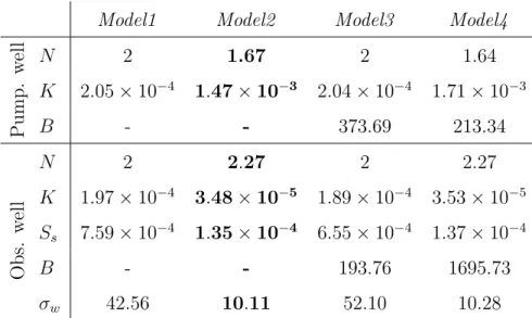
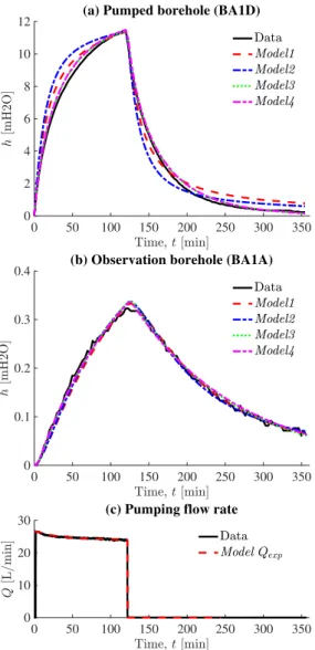
Figure 4: Data and models related to experiment Exp1A. The results obtained with the following models overlap: (a) Model1 Model3 and Model2 Model4, (b) Model2 Model3 -Model4.
Model1 Model2 Model3 Model4 Pump. w ell N 2 1.67 2 1.64 K 2.05 × 10⁻⁴ 1.47 × 10⁻³ 2.04 × 10⁻⁴ 1.71 × 10⁻³ B - - 373.69 213.34 Obs. w ell N 2 2.27 2 2.27 K 1.97 × 10⁻⁴ 3.48 × 10⁻⁵ 1.89 × 10⁻⁴ 3.53 × 10⁻⁵ Ss 7.59 × 10⁻⁴ 1.35 × 10⁻⁴ 6.55 × 10⁻⁴ 1.37 × 10⁻⁴ B - - 193.76 1695.73 σw 42.56 10.11 52.10 10.28
Table 3: Properties estimated for the models and data presented in Figure 4 (Exp1A).
3.1.2. Pumping test in borehole BA1D
334
In experiment Exp1D, the pumping was applied in borehole BA1D for
335
355 minutes and the flow rate decreased from 26.7 to 24.1 L/min (Figure 5c).
336
The collected data and the corresponding acceptable models are shown in
337
Figure 5 and Table 4. As for Exp1A, a common model reproducing the
338
data collected in both the pumped and observation boreholes could not be
339
found. Concerning the data collected in the pumped borehole (Figure 5a),
340
Model1 and Model3 provide an acceptable fit and the transmissivity value
341
estimated with Model1 is consistent with that of Theis’ method, which is
342
equal to 2.15 × 10⁻⁵ m2/s. The best fit is obtained with Model3, whereas
343
Model2 does not provide an acceptable fit and Model4 does not improve the
344
results obtained with Model3. These results show the importance of leakage
345
processes for reproducing the data observed in borehole BA1D, as well as
346
the presence of open fractures that intersect the well (N = 2 and σw < 0 for
Ss < 3 × 10⁻² m−1 from additional simulations).
348
Regarding the data collected in the observation borehole, we obtain a
349
correct fit with all the models, whereas interpreting the end of the recovery
350
with Theis’s method is not possible because the recovery is not developed
351
enough. Model3 is considered as the best-fitting model because the large
352
values of skin factor in Model1 and Model2 are not realistic and Model4 does
353
not improve the results.
354
Model1 Model2 Model3 Model4
Pump. w ell N 2 1.83 2 2 K 2.02 × 10⁻⁵ 1.61 × 10⁻⁴ 4.5 × 10⁻⁶ 4.47 × 10⁻⁶ B - - 31.04 31.04 Obs. w ell N 2 1.8 2 1.45 K 3.21 × 10⁻⁴ 1.19 × 10⁻³ 3.96 × 10⁻⁶ 2 × 10⁻⁵ Ss 3.08 × 10⁻⁴ 1.12 × 10⁻³ 2.9 × 10⁻⁵ 1.43 × 10⁻⁴ B - - 5 4 σw 206.91 594.53 1.39 54
Table 4: Properties estimated for the models and data presented in Figure 5 (Exp1D ).
3.2. Multi-level pumping tests
355
3.2.1. Pumping tests in borehole BA1A
356
The multi-level pumping experiments conducted in borehole BA1A lead
357
to the data and models shown in Figure 6 and Table 5 for experiment
358
Exp2A i1A and Figure 7 and Table 6 for experiment Exp2A i2A. No
re-359
sults are presented for experiment Exp2A i3A because it was not possible
360
to pump in the considered interval (133-400 m). In this case, we estimate
0 50 100 150 200 250 300 350 0 2 4 6 8 10
12 (a) Pumped borehole (BA1D)
0 50 100 150 200 250 300 350 0
0.1 0.2 0.3
0.4 (b) Observation borehole (BA1A)
0 50 100 150 200 250 300 350 0
10 20
30 (c) Pumping flow rate
Figure 5: Data and models related to experiment Exp1D. The results obtained with Model3 and Model4 overlap.
that the transmissivity of this zone is smaller than 7 × 10⁻⁸ m2/s, which
362
is the smallest transmissivity in which we could pump with that pumping
363
equipment.
364
In experiment Exp2A i1A, a multiple-step pumping flow rate is applied
(Figure 6c). The data collected in the pumped (Figure 6a) and observation
366
(Figure 6b) wells are interpreted by dividing the pumping flow rate data into 5
367
sub-steps in order to account as thinly as possible for the flow rate variations,
368
and are modeled by considering flow-rate-dependent values of the skin factor
369
σw (Figure 6d). Note that the flow-rate dependence of the skin factor has
370
been observed and studied in previous work, in particular in step-drawdown
371
tests (Jacob, 1947; Rorabaugh, 1953; van Everdingen, 1953; Kruseman and
372
de Ridder, 1990). Furthermore, the model parameters provided in Table 5
373
are characteristic of flow in fractured media with σw < 0 when N = 2 for
374
Model1 and Model3 and N = 1 for Model2 and Model4.
375
The flow dimension of Model2 and Model4 indicates the presence of a
376
channel, or several independent channels, that dominate the flow. The high
377
values of σw estimated with these models show either (i) clogging of the
378
channel that intersects the pumping well or (ii) the channel does not intersect
379
the pumping well and hydraulic connection occurs through permeable porous
380
media or fissures. Note that the high values of σw can be explained by the
381
fact that the interpretation of the skin factor with the generalized radial flow
382
model is not explicit when N 6= 2 because the pumping chamber geometry of
383
the model does not correspond to its real geometry. The difference between
384
these two geometries impacts the value of the skin factor, which could explain
385
why high values of the skin factor can be found for low flow dimension (Hamm
386
and Bidaux, 1996; Lods and Gouze, 2004). Model2 is selected as the most
387
realistic model because (i) it provides a much better fit with the collected
388
data than Model1 with an almost-linear increase of the skin factor and (ii)
389
Model3 and Model4 do not improve the results obtained with Model2. The
transmissivity values estimated with Theis’ method are 5 times greater than
391
those obtained for the pumped and observation boreholes with Model1, which
392
is explained by the inadequacy of Model1.
393
Model1 Model2 Model3 Model4
N 2 1 2 1
K 2.37 × 10⁻⁵ 1.6 × 10⁻² 2.31 × 10⁻⁵ 1.56 × 10⁻² Ss 1.12 × 10⁻³ 1.1 × 10⁻¹ 1.1 × 10⁻³ 1.09 × 10⁻¹
B - - 55.57 172.79
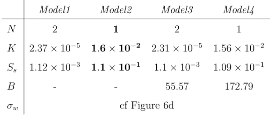
σw cf Figure 6d
Table 5: Properties estimated for the models and data presented in Figure 6 (Exp2A i1A).
For experiment Exp2A i2A, a common model reproducing the data
col-394
lected in the pumped and observation boreholes could not be found. The
395
results presented in Figure 7 and Table 6 show that the fit to the data that
396
is obtained with Model1 can be improved with Model3, whereas Model2 and
397
Model4 do not improve these results. The transmissivity values estimated
398
with Theis’s method are equal to 1.06 × 10⁻⁵ m2/s and 3.94 × 10⁻⁵ m2/s for
399
the pumped and observation boreholes, respectively, corresponding to larger
400
and smaller values, respectively, than that obtained with Model1.
401
3.2.2. Pumping tests in borehole BA1D
402
The data and models related to the multi-level pumping tests conducted
403
in borehole BA1D are shown in Figure 8 and Table 7 for experiment Exp2D i1D,
404
Figure 9 and Table 8 for experiment Exp2D i2D, and Figure 10 and Table 9
405
for experiment Exp2D i3D. For experiments Exp2D i1D and Exp2D i2D, a
406
common model could not be found to reproduce the data collected in both
0 100 200 300 400 0 0.5 1 1.5 2
2.5 (a) Pumped borehole (BA1A)
0 100 200 300 400 0 0.2 0.4 0.6 0.8
1 (b) Observation borehole (BA1D)
0 100 200 300 400
0 10 20
30 (c) Pumping flow rate
5 10 15 20 -5 -4 220 280 340
(d) Estimated skin factor, w [-]
Figure 6: Data, models, and parameters related to experiment Exp2A i1A. (a-b) The results obtained with the following models overlap: Model1 -Model3 and Model2 -Model4. In (d) the changes in the esti-mated skin factor σwwith the step average flow rate ¯Q are shown for Model1 -Model3 (red crosses-green
0 50 100 150 200 250 300 0
10 20 30
40 (a) Pumped borehole (BA1A)
0 50 100 150 200 250 300 0 0.1 0.2 0.3 0.4
0.5 (b) Observation borehole (BA1D)
0 50 100 150 200 250 300 0
5
10 (c) Pumping flow rate
Figure 7: Data and models related to experiment Exp2A i2A.
the pumped and observation boreholes, implying that the models are defined
408
for each borehole. For experiment Exp2D i3D, no response was observed in
409
the observation borehole implying that the models are only defined for the
410
pumped borehole.
411
Concerning experiment Exp2D i1D, the results reported in Figure 8a and
Model1 Model2 Model3 Model4 Pump. w ell N 2 2.1 2 2 K 6.15 × 10⁻⁶ 4.59 × 10⁻⁶ 2.74 × 10⁻⁶ 2.65 × 10⁻⁶ B - - 28.53 22.41 Obs. w ell N 2 2.2 2 1.2 K 5.6 × 10⁻⁵ 1.54 × 10⁻⁵ 2.5 × 10⁻⁵ 10−2 Ss 2.41 × 10⁻⁴ 9.74 × 10⁻⁵ 3.24 × 10⁻⁴ 8.64 × 10⁻³ B - - 24.88 111.24 σw 0 0 0 −2.9 × 10⁻⁴;−7 × 10⁻⁵
Table 6: Properties estimated for the models and data presented in Figure 7 (Exp2A i2A).
Table 7 show that Model1 and Model2 do not provide an acceptable fit of
413
the recovery data recorded in the pumped borehole, whereas Model3 and
414
Model4 fit well the data. The best-fitting model (Model4 ) corresponds to a
415
non-cylindrical flow that is dominated by a channel (N = 1) with important
416
leakage (B = 2.92). Additional simulations show that σw < 0 when Ss <
417
2×10⁻¹m−1, which indicates the presence of open fractures that intersect the
418
well. Similar results are observed for the data collected in the observation
419
borehole since the fit obtained with Model1 could not be improved with
420
Model2 whereas Model3 and Model4 fit well the data, the best fit being
421
obtained with Model4 (Figure 8b). In this case, σwhas no effect on the results
422
(σw = 0), implying that the estimated values of K/Ss and Ssare reliable, the
423
high values of Ss being characteristic of semi-confined aquifers. Finally, the
424
hydraulic conductivity values estimated with Model1 are consistent with the
425
transmissivity values obtained using Theis’ method, which give 5.53 × 10⁻⁶
and 1.37 × 10⁻⁴ m2/s for the pumped and observation well, respectively. 0 500 1000 1500 2000 0 5 10 15
20 (a) Pumped borehole (BA1D)
0 500 1000 1500 2000 0 0.1 0.2 0.3 0.4 0.5
0.6 (b) Observation borehole (BA1A)
0 500 1000 1500 2000
0 10 20
30 (c) Pumping flow rate
Figure 8: Data and models related to experiment Exp2D i1D.
427
When studying the interval 102-132 m (experiment Exp2D i2D ), we
con-428
sider the four-step pumping flow rate presented in Figure 9c. Figure 9a shows
429
that Model1 and Model2 do not fit the recovery, whereas Model3 and Model4
430
provide a perfect fit to the data collected in the pumped borehole, resulting
Model1 Model2 Model3 Model4 Pump. w ell N 2 2.05 2 1 K 9.4 × 10⁻⁶ 1.06 × 10⁻⁵ 3.94 × 10⁻⁶ 1.3 × 10⁻⁴ B - - 17.13 2.92 Obs. w ell N 2 1.89 2 1.67 K 1.92 × 10⁻⁴ 3.68 × 10⁻⁴ 1.84 × 10⁻⁴ 1.26 × 10⁻³ Ss 1.38 × 10⁻³ 2.49 × 10⁻³ 1.34 × 10⁻³ 7.83 × 10⁻³ B - - 197.35 105.4 σw 0 0 0 0
Table 7: Properties estimated for the models and data presented in Figure 8 (Exp2D i1D ).
in considering the simplest model (i.e., Model3 ) as the best-fitting model.
432
For the data collected in the observation borehole, all models provide an
433
acceptable fit to the data, implying that the simplest model (i.e., Model1 )
434
is considered as the best-fitting model. In the case of the pumped-borehole
435
models, the decrease in the slope of σw versus ¯Q when ¯Q = 1.79 L/min
(Fig-436
ure 9d) is characteristic of unclogging phenomena, while the good fit between
437
the collected and simulated data suggests that these phenomena are
local-438
ized in the borehole skin. Additional analyses point out that σw is negative
439
only when Ss is smaller than 1.9 × 10⁻⁵ m−1, which indicates the absence of
440
fractures that intersect the wells with apertures larger than in the formation.
441 442
Because of the low permeability of the interval 133-400 m (experiment
443
Exp2D- i3D ), very small flow rates were applied when studying this zone
444
(Figure 10b). During this experiment, no response was recorded in the
0 100 200 300 400 0
5 10 15
20 (a) Pumped borehole (BA1D)
0 100 200 300 400 0 1 2 3 4 5 6
(b) Observation borehole (BA1A)
0 100 200 300 400
0 2 4
(c) Pumping flow rate
0.5 1 1.5 2 2.5 3
-5 0
5 (d) Estimated skin factor
Figure 9: Data and models related to experiment Exp2D i2D. The results obtained with the following models overlap: (a) Model1-Model2 and Model3-Model4, (b) Model1-Model3 and Model2-Model4. In (d) the changes in the estimated skin factor σw with the step average flow rate ¯Q are shown for Model1 (red
Model1 Model2 Model3 Model4 Pump. w ell N 2 2 2 2 K 4.5 × 10⁻⁶ 4.5 × 10⁻⁶ 2.49 × 10⁻⁶ 2.49 × 10⁻⁶ B - - 10.03 10.03 Obs. w ell N 2 1.51 2 1.51 K 1.79 × 10⁻⁴ 3.79 × 10⁻³ 1.79 × 10⁻⁴ 3.79 × 10⁻³ Ss 1.54 × 10⁻³ 1.89 × 10⁻² 1.54 × 10⁻³ 1.89 × 10⁻² B - - - -σw 0 0 0 0
Table 8: Properties estimated for the models and data presented in Figure 9 (Exp2D i2D ).
servation borehole BA1A and the small flow rates were difficult to apply and
446
maintain, resulting in irregular initial flow rates. In this case, the response
447
recorded in the pumped borehole is interpreted by dividing the pumping flow
448
rate data into 9 sub-steps. The results shown in Figure 10a and Table 9 are
449
obtained by using, as before, a step-wise exponential model to reproduce the
450
pumping flow rate in Model1, Model2, Model3 and Model4 (dashed red curve
451
in Figure 10b). In order to demonstrate the importance of this exponential
452
model, we also show the results obtained with Model3’, which considers a
453
step-wise constant pumping flow rate (dash-dot blue curve in Figure 10b).
454
These results show that Model1 does not provide an acceptable fit to the data
455
because, namely, of an important increase in the drawdown at the beginning
456
of the last pumped steps. Attempt to reduce these peaks leads to models
457
with unrealistic values of the wellbore storage coefficient (not shown). On
458
the contrary, these peaks are eliminated with Model2, Model3 and Model4,
Model3 being the best-fitting model. The transmissivity value estimated
460
with Model1 is consistent with that of the standard Theis’ method, which
461
is equal to 6.71 × 10⁻⁸ m2/s. Furthermore, Figure 10c shows that
increas-462
ing ¯Q from 0.079 to 0.267 L/min with Model1, Model2, Model3 and Model4
463
results in decreasing σw. This behavior is characteristic of the occurrence
464
of an unclogging phenomenon. On the contrary, when using Model3’, this
465
skin factor behavior is not observed (not shown) and a large discrepancy
466
is observed during the recovery between the simulated and collected data
467
(dotted balck curve in Figure 10a), demonstrating the importance of using a
468
step-wise exponential model for representing the pumping flow rate.
Model1 Model2 Model3 Model4
N 2 2.99 2 2.09
K 6.99 × 10⁻⁸ 1.32 × 10⁻⁸ 2.3 × 10⁻⁸ 2.11 × 10⁻⁸
B - - 0.21 0.26
Table 9: Properties estimated for the models and data presented in Figure 10 (Exp2D i3D ).
469
3.3. Cross-borehole multi-level-monitoring pumping experiment
470
In experiment Exp3D, a pumping flow rate of 20.17 L/min was applied
471
during 338 min in borehole BA1D while monitoring the pressure in the
in-472
tervals i1A0 (22-107 m), i2A (108-132 m), and i3A (133-400 m) in borehole
473
BA1A (Figure 11). Here, the data cannot be interpreted with the models
474
presented before because the flow rate applied to each interval is not known.
475
The data collected during this experiment are rather used to confirm and
476
complete the information previously obtained on the connections between
0 50 100 150 200 0 10 20 30 40
50 (a) Pumped borehole (BA1D)
0 50 100 150 200
0 1
2 (b) Pumping flow rate
0.05 0.1 0.15 0.2 0.25 0.3 0.35 -0.8
-0.2
0.4 (c) Estimated skin factor
Figure 10: Data, models, and parameters for experiment Exp2D i3D. In (c) the changes in σwwith the step average flow rate ¯Q are shown for Model1 (red crosses), Model2 (blue circles), Model3 (green triangles) and Model4 (magenta squares).
the pumped and observation boreholes, as well as between various intervals
478
of these boreholes.
479
From the data reported in Figure 11, we determine that the reaction
480
times of intervals i1A0, i2A, and i3A are 4, 1, and 9 min, respectively. These
481
observations can be related to the results presented in Section 3.2.1 where the
482
multi-level pumping tests conducted in borehole BA1A are interpreted with
483
various models. Using Model1 leads to show that (i) the diffusivity estimated
in interval i1A is smaller than that of interval i2A since K/Ss = 2.12 ×
485
10−2 m2/s in Exp2A i1A, and 2.16 × 10⁻¹ (pumping borehole) and 2.32 ×
486
10−1 m2/s (observation borehole) in Exp2A i2A, and (ii) the transmissivity
487
of i3A is below the capability of our pumping equipment since it was not
488
possible to pump in Exp2A i3A. Considering that interval i1A is included
489
into i1A0, the reaction times defined from experiment Exp3D are consistent
490
with the results from experiments Exp2A.
491
The reaction of interval i3A reported in Figure 11 also indicates that
492
there is a connection between this interval and borehole BA1D whereas the
493
results of Exp2D i3D show that this interval is not hydraulically connected
494
to interval i3D of borehole BA1D. This demonstrates that interval i3A is
495
connected to borehole BA1D through non-horizontal flow. This is consistent
496
with the leakage models of experiments Exp2D i2D and Exp2D i3D, which
497
result in the presence of vertical flow between intervals i2D and i3D.
0 50 100 150 200 250 300 350 0 0.5 1 1.5 2 2.5 3
Figure 11: Data monitored in intervals i1A0, i2A and i3A of the observation borehole BA1A while pumping in borehole BA1D (experiment Exp3D ).
4. Discussion
499
The parameters inferred from modelling the pumped well drawdown
re-500
veal the hydraulic properties in the vicinity of the pumping well. Conversely,
501
those evaluated from the observation well data are effective parameters
in-502
tegrating all the hydraulic structures from surface to depth including local
503
draining zones. Nevertheless, the parameters evaluated at the observation
504
well, when different from those inferred at the pumping well, enlighten the
505
heterogeneity and probable anisotropy of the studied system.
506
Figure 12 summarizes the main conclusions that are obtained from the
507
(non-unique) models presented in Section 3, including the open-borehole tests
508
Exp1A and Exp1D and the cross-borehole multi-level hydraulic experiments
509
Exp2A and Exp2D. Interpreting the open-borehole tests Exp1A and Exp1D
510
with Model1 leads to a transmissivity of BA1D one order of magnitude lower
511
than that of BA1A with leakage in the former case. These results, which are a
512
first indication of the horizontal and vertical heterogeneities that characterize
513
the system, are consistent with the open-borehole experiments in Dewandel
514
et al. (2005) that could be interpreted with N = 2. Furthermore, in the
515
case of Exp1D, the need for considering important leakage processes can be
516
related to the presence of an overlying aquifer zone located above BA1D
517
casing base depth, in the alluvium (Figure A.16), at which a productive
518
interval (26-27 m) is detected by the flowmeter (Figure A.14c).
519
Concerning the cross-borehole multi-level hydraulic experiments Exp2A
520
and Exp2D, the presented results emphasize the strong variability of the
hy-521
draulic properties induced by the heterogeneities of the geological structures.
522
For the upper part of the system (i.e., intervals i1A and i1D located between
41 and 75 m), results indicate the presence of highly conductive fractures
524
(N < 2 in Exp2A i1A and Exp2D i1D ) with different behaviors
depend-525
ing on the considered pumped borehole. When pumping in borehole BA1A
526
(Exp2A i1A), a unique model with N = 1 is found to interpret the data
col-527
lected in both boreholes. This shows that the hydraulic responses of BA1A
528
and BA1D are driven by a highly conductive channelized structure (N = 1),
529
for example an extended, open or partially mineralized fracture within which
530
a 1D channel is developed. The two boreholes do not necessarily intersect
531
the channel, they can be connected to it by a conduct in which the flow
532
rate becomes rapidly permanent. On the contrary, when pumping in BA1D
533
(Exp2A i1D ), two different leakage models are required to describe the data
534
collected in the boreholes with an increase in the hydraulic conductivity and
535
flow dimension from the pumped to the observation-borehole model. In this
536
case, the need for leakage models with high values of the leakages for the
537
pumped-borehole model, as well as the heterogeneities in properties between
538
the boreholes with N > 1 for the observation-borehole model, show that the
539
hydraulic responses are only partially determined by the highly conductive
540
channelized structure previously described. That is, the water pumped in
541
the upper tested interval of BA1D comes from the highly conductive
chan-542
nelized structure previously described that connect the upper intervals of the
543
considered boreholes (horizontal connections), but also from underlying and
544
overlying rocks surrounding BA1D (vertical connections). Thus additional
545
vertical flow contributions are present when pumping in BA1D, whereas the
546
horizontal connections are sufficient for the pumping in BA1A with similar
547
pumping flow rates.
Concerning the middle part of the system (i.e., intervals i2A and i2D
549
located between 102 and 132 m), the value of the estimated flow
dimen-550
sion (N = 2) for the pumped and observation boreholes in Exp2A i2A and
551
Exp2D i2D, shows that the observed hydraulic responses are not determined
552
by the presence of conductive structures with channelized flow as for the
553
upper part of the system. Conversely, these models are related to leakage
554
properties except for the observation-borehole model of Exp2D i2D for which
555
a high value of the hydraulic conductivity is obtained (K = 1.8 × 10⁻⁴ m/s).
556
This indicates the presence of heterogeneities in the directions of the flows
557
that contribute to the pumping: (i) the pumping in BA1A is supplied by
558
both horizontal and vertical flows that are located around and far from the
559
pumped borehole, and (ii) the pumping in BA1D is supplied by horizontal
560
and vertical flows close to the pumped borehole, and only horizontal flows
561
around borehole BA1A. This might be related to the location of BA1A for
562
which highly conductive structures of the upper part of the system was
de-563
tected (see above). Indeed, considering that BA1A is surrounded by these
564
structures, one can speculate that they contribute to the water pumped in
565
BA1D by flowing from the upper to the middle part of the system through
566
borehole BA1A and flowing horizontally in the middle part of the system
567
from BA1A to BA1D. This explains that there is no vertical flow around
568
BA1A when pumping in BA1D and that there is no counterpart behavior
569
observed when pumping in BA1A.
570
Finally, the pumping experiments conducted by isolating the lower part
571
of the system (i.e., intervals i3A and i3D located between 133 and 400 m)
572
also show a potential impact of the localization of the wells regarding the
conductive structures of the system. Whereas it was not possible to pump
574
water from BA1A (Exp2A i3A) because the transmissivity of this layer was
575
too low, we observe a different behavior in BA1D for which the data
col-576
lected in the pumped borehole are well described with a leakage model
577
(Exp2D i3D ). In this case, the pumped water is supplied by vertical
con-578
nections occurring around the pumped borehole, which are coming from the
579
middle part of the system that is located directly above the considered area
580
(i.e., without intermediary poorly-permeable zones) and connected to the
581
upper highly transmissive part of the system through BA1A. The differences
582
between Exp2A i3A and Exp2D i3D can be explained by heterogeneities in
583
the vertical hydraulic properties implying that there is no flow exchanges
be-584
tween the middle and lower parts of the system in the former case, whereas
585
these exchanges occur in the latter.
586
5. Conclusions
587
The cross-borehole multi-level hydraulic experiments presented in
Sec-588
tion 3 show a complex behavior of the ophiolitic hard-rock aquifer located
589
within the BA1 site of the Sultanate of Oman. The discussion provided
590
in Section 4 explains this behavior by the presence of highly transmissive
591
structures in the upper part of the system and different locations of the
592
boreholes into these structures, resulting in strong geological and hydraulic
593
heterogeneities in all directions. Within a 15 m area, this study reveals
de-594
grees of heterogeneities going from 1D channelized flows sparsely connected
595
to far-field resources to 2D standard systems supplied by nearby surrounding
596
zones.
The characterization previously described required to conduct hydraulic
598
tests in zones with variable permeability going from highly to poorly
con-599
ductive areas. In the latter case, pumping at very small flow rates (smaller
600
than 1 L/min) is a technical challenge for which decreasing flow rates cannot
601
be avoided. Whereas this behavior has never been considered in the data
602
interpretation of existing studies, we developed models that are able to take
603
into account this feature, and we show that this characteristic of the pumping
604
flow rate is critical for interpreting the experiments.
605
The experiment interpretation was done using four transient radial
so-606
lutions relying on various assumptions going from cylindrical flow without
607
leakage to generalized radial flow with leakage. We believe that the data
608
analysis methodology and the parameter estimation strategy developed for
609
this work should be useful for interpreting other pumping experiments
specif-610
ically in low permeability heterogeneous systems and when vertical leakages
611
are important. In addition, the efficiency of these semi-analytical models
612
makes them an ideal tool for conducting parametric sensitivity analysis and
613
inverting experimental data in the context of complex parameter sets.
614
The use of fractional flow models is justified in this work by direct
geolog-615
ical observations and the need to consider vertical leakages, and confirmed by
616
the satisfying curve-fitting and coherent parameter and property estimates.
617
Despite the fractured nature of ophiolitic aquifers, the adequacy of the
dual-618
permeability concept for describing these systems is an open question, in
619
particular because there is no evidence of large-scale fractures embedded
620
into a poorly-permeable matrix as observed for granitic systems. The doubt
621
about a potential dual-permeability behavior of ophiolitic aquifers requires to
integrate vertical leakages in such models and to collect additional data such
623
as breakthrough curves from chemical tracer experiments. Future work for
624
the site considered in this study will focus on this characterization method
625
with the objective of improving our ability to characterize ophiolitic aquifers
626
and understanding their behavior.
627
Notations
628
Ss Aquifer specific storage [m−1]
K Hydraulic conductivity [m s−1]
T = bK Transmissivity [m2 s−1]
B Leakage factor [m]
β Leakage parameter [m−2]
h Drawdown [m]
r Distance from the well [m]
N Flow dimension [-]
rw Well-aquifer exchange radius [m]
b Ortho-radial extent [m]
Sw Well storage coefficient [m2]
σw Skin factor [-]
Q Pumping flow rate [m3 s−1]
¯
Q Pumping step average flow rate [m3 s−1]
629
Acknowledgments
630
We would like to thank Prof. Peter Kelemen, Prof. Damon Teagle and
631
Dr. Jude Coggon for their overall support, and Eng. Zaher Al Sulaimani,
632
Mazin Al Sulaimani from the Oman Water Centre and AZD Engineering,
Figure 12: Summary of the mo dels and prop erties estimated from the pu m p ing exp erimen ts Exp1A , Exp1D , Exp2A and Exp2D . The n um b ers written in italic denote the distance from the surface. K and N are the h ydraulic conductivit y (in m/s) and flo w dimension, res p ectiv ely , estimated with the b est-fitting mo del of eac h exp erimen t. F or eac h exp erimen t, the v alue of K estimated with Mo del1 is also pro vided (v alue in brac k ets) in order to compare th e in tegrated conductiv e prop erties . The thic kness of the red ar ro w characterizes the imp ortance of the leak age pro cess .
Eng. Said Al Habsi, Dr. Rashid Al Abri, Eng. Salim Al Khanbashi, Eng.
634
Haider Ahmed Mohammed Alajmi, Mohsin Al Shukaili, Salim, Al Amri, and
635
Ali Al Shukaili from the Ministry of Regional Municipalities and Water
Re-636
sources for logistical and technical support during the borehole testing. We
637
also thank Prof. Martin Stute and Prof. Amelia (Paukert) Vankeuren for
ex-638
perimental assistance, and Dr. Marguerite Godard for her helpful comments
639
on the manuscript and for the edition of Figure 1. Funding for this study was
640
provided by the International Continental Scientific Drilling Program to the
641
Oman Drilling Project, and the Alfred P. Sloan Foundation (Grant
2014-3-642
01) and U.S. NSF (Grant NSF-EAR-1516300) to Columbia University, New
643
York.
Appendix A. Additional data
645
Vertical heterogeneities of boreholes BA1A and BA1D were investigated
646
by measuring the temperature profiles in the boreholes (Figure A.13) and
647
conducting flowmeter tests under ambient and forced hydraulic conditions
648
(Figure A.14). The temperature profiles are obtained with the multi
pa-649
rameter probe ALT QL40 OCEAN, which allows measuring temperature
650
between 0 and 50 ◦C, and the flowmeter data are obtained with the heat
651
pulse flowmeter Mount Sopris HFP-2293, which allows measuring flow rates
652
between 0.1 to 4 L/min. The data obtained under forced hydraulic
condi-653
tions were collected while pumping at a flow rate of 18.12 and 4.47 L/min in
654
boreholes BA1A and BA1D, respectively. The full temperature profiles show
655
temperature anomalies for both boreholes above 61 m (Figure A.13a), and
656
their enlargement between 115 and 155 m shows a temperature anomaly at
657
depth 130-131 m in borehole BA1A (Figure A.13b). From the flowmeter data
658
collected in borehole BA1A, we observe changes in the vertical flow rates at
659
depth 22-29 m in Figure A.14a and at depth 33-39, 45-46 and 58-59 m in
660
Figure A.14b. Finally, the flowmeter data collected in borehole BA1D and
661
displayed in Figure A.14c show changes in the vertical flow rates at depth
662
26-27, 62-64 and 105-130 m. These conductive zones are reported in
Ta-663
ble A.10 with the corresponding intervals that are considered for the packer
664
experiments in order to characterize these zones. The isolated intervals are
665
chosen such that they include the conductive zones and they are located at
666
comparable positions for both boreholes.
667
While conducting the packer experiments, the pressure changes above
668
and below the isolated intervals are monitored. These pressures, denoted
32 36 40 44 0 50 100 150 200 250 300 350 400 (a) 0-400 m 35 36 37 115 120 125 130 135 140 145 150 155 (b) 115-155 m
Figure A.13: Temperature profile in boreholes BA1A and BA1D (a) from 0 to 400 m and (b) from 115 to 155 m depth, showing an anomaly in temperature at depth 130-131 m in borehole BA1A.
-20 0 20 20 25 30 35 40 45 50 55 60 65 (a) -2 0 2 30 35 40 45 50 55 60 65 (b) 0 5 20 40 60 80 100 120 140 (c)
Figure A.14: Flowmeter data collected under ambient (blue crosses and dashed lines) and forced (red circles and dotted lines) hydraulic conditions in boreholes (a-b) BA1A and (c) BA1D. Symbols and (dashed and dotted) lines correspond to raw and interpreted data, respectively. The black line represent zero values of flowrate. (b) corresponds to a zoom-in of (a) for interpretation purpose. The values monitored below 65 m in (a-b) and below 140 m in (c) are null (and not shown).
P1 (below) and P3 (above), are reported in Figure A.15 for experiments
670
Exp2A i1A, Exp2A i2A, Exp2D i1D and Exp2D i2D. The pressures are not
671
shown for experiments Exp2A i3A since the pumping could not be applied,
672
and Exp2D i3D because P1 is not recorded for the interval located at the