WITH THE NATURAL GAS SHORTAGEI by Paul W. MacAvoy 659 - 73 ** Robert S. Pindyck June, 1973
* Professor of Economics, Sloan School of Management, Massachusetts Institute of Technology
** Assistant Professor of Economics, Sloan School of Management, Massachusetts Institute of Technology
develop an Econometric Policy Model of Natural Gas, under National Science Foundation Grant #GI-34936. The Phase I version is reported in Sloan School of Management Working Paper #635-72 (December 1972), and the Phase III
version, a Domestic United States Oil and Gas Policy Model, will be com-pleted by July, 1974. Comments are invited on this interim version.
The results of this project would not have been possible without the support of our research assistants at M.I.T. We would like to extend our sincere appreciation to Robert Brooks, Krishna Challa, Ira Gershkoff, Marti Subrahmanyam and Philip Sussman for their energetic and enthusiastic help in developing a computerized data base during the summer of 1972, and esti-mating and simulating the model over the past few months. They worked many long hours, and often under considerable time pressure. We received con-siderable support from the National Bureau of Economic Research Computer Center in the use of the TROLL system for the estimation and simulation of
the model, as well as the maintenance of our data base. We would like to thank Mark Eisner, Fred Ciarmaglia, Richard Hill, and Jonathan Shane for their help in using TROLL. We would also like to express our appreciation to Morris Adelman and Gordon Kaufman of M.I.T., and Robert Fullen and Wade Sewell of the Federal Power Commission for their comments and suggestions. Commissioner Nassikas of the F.P.C., Mr. Charles DiBona of the White House Staff, and staff members of the Senate Commerce Committee were of substantial assistance in formulating policy alternatives. Finally, more than six dozen
readers of the Phase I version of the model provided critical comments neces-sary for reformulating the model along the lines presented below. We are obligated to them all, and absolve them from responsibility for the results by granting them anonymity.
Low wellhead ceiling prices over the past decade have led to the beginning of a shortage in natural gas production. If the demand for gas grows as expected during the 1970's, and if ceiling prices remain low as a result of restrictive regulatory policy, this shortage could grow significantly. This paper examines the effects of this and alter-native regulatory policies on gas reserves, production supply, production demand, and prices over the remainder of this decade. An econometric model is developed to explain the gas discovery process, reserve accu-mulation, production out of reserves, pipeline price markup, and whole-sale demand for production on a disaggregated basis. By simulating this model under alternative policy assumptions, we find that the gas shortage
can be ameliorated (and after four or five years eliminated) through phased deregulation of wellhead sales, or through new regulatory rulings, either of which imply moderate increases in the wellhead price for new con-tracts. These results are also rather insensitive to alternative forecasts of such exogenous variables as GNP growth, population growth, and changes in the prices of alternate fuels.
1.1 Introduction
A substantial shortage of natural gas has been developing over the last few winter heating seasons. Reports of the Federal Power Commission
indicate that in the winters of 1970 to 1972 gas supplies were cut off with increasing frequency, and for longer periods of time, throughout the North
1
and Eastern portions of the United States. This has been a matter not only of cutting off supplies in peak periods to industry -- as occurred in Cleveland in January 1970 when 30,000 employees of 700 companies were laid off for 10 days as a result of gas interruptions -- but of systematic curtailments of deliveries to certain classes of consumers. During 1971-1972, seven major interstate pipelines curtailed service throughout the winter season to existing customers. Service entering the Northeastern part of the country from Texas Eastern Transmission Corporation was
cur-tailed 18 percent, from Transcontinental Gas Pipeline 9 percent, and from Trunkline Gas Company 27 percent. Service throughout the region from New Mexico to Southern California was curtailed by El Paso Natural Gas Company by 15 percent. The Federal Power Commission staff has shown deliveries
falling short of the amount of gas demanded for consumption by 3.6% in 1971 and by 5.1% in 1972, and has predicted that production will fall short of demand by 12.1% by 1975.
1Federal Power Commission, Proceedings on Curtailment of Gas Deliveries of
Interstate Pipelines (1972).
2
Federal Power Commission, Bureau of Natural Gas, Natural Gas Supply and Demand 1971-1990 (1972), p. 123.
These estimates encompass recent and expected future production shortages. The amounts do not include anywhere near all of the unsatis-fied demands for gas. The "markets" for natural gas are not spot markets for production, but rather center on sales of reserves. The pipeline buyer offers to take new gas deposits out of the ground, and pays for this production, so as to deliver gas to residential, commercial and industrial
consumers throughout the United States. The transaction involves the dedication of reserves by oil and gas discovery companies to pipelines, and this is followed by a transaction in which the pipelines make commit-ments to deliver production to final consumers over a ten to twenty year
period. The reserves markets have experienced shortages to a much greater extent than shown by recent production shortages (according to one estimate, new reserves have been more than 50 percent short since 1961 ). Also, it has been estimated that demands for new production by both old and new potential buyers together exceeded the total supply of new production available by more than 50%.2 These unsatisfied demands were never regis-tered by curtailment proceedings because most of the new potential buyers did not receive new service from the pipelines. This shortage was realized
The estimate was obtained from a four-equation supply and demand model of natural gas reserves constructed on the basis of data over the 1950's and fitted to values of the exogenous variables over the 1960's. The difference between the fitted values of reserves those that would clear the market --and the actual valuesof reserves made available in fuel producing markets to go to the East Coast and Midwest was more than 50% of fitted reserves each year from 1961 to 1968. Cf. S. Breyer and P. MacAvoy, "The Natural Gas Shortage and the Regulation of Natural Gas Producers," Harvard Law Review, 86: 941-987 (1973), pp. 968-976.
in additional demands for other fuels with less satisfactory burning and air polluting characteristics.
Production curtailments have immediate effects on the consumer,
requiring him to use stand-by heating facilities or possibly to do without heating entirely. The larger shortage of new production contract commit-ments has more diverse effects. Some consumers are required to go to other fuels -- with the result that their consumption costs are increased, or that pollution is greater so that social costs are increased. Other consumers can work their way around the shortage by changing locations or by offering various premia to be put at the head of the queue. In general, the economic and locational effects of the shortage are likely to be significant.1
The political consequences are another matter. The contract sales of gas at the wellhead and at the city gate are closely regulated by the Federal Power Commission, so that the F.P.C., the Congress, and the Office
of the President become focal points for complaints that regulatory poli-cies have either caused or failed to ameliorate the shortages. With neither producers nor consumers supporting the regulatory process -- neither clearly benefiting from the shortage -- the possibility of significant political losses for legislators or regulators is substantial.
1An initial attempt is made in Breyer and MacAvoy to measure the economic
effects of the shortage on consumers. It is argued there that the reserve shortage is incurred by residential and commercial consumers buying from regulated interstate pipelines, while industrial consumers buying in unre-gulated transactions do not experience the shortage to the same extent. Because of the magnitude of the amounts short in the 1962-1968 period, final residential and commercial consumers are believed to have been made worse off as a group from a combination of lower regulated prices and large
shor-tages. Cf. Breyer and MacAvoy, op. cit. No attempt is made here to refine these estimates with the more advanced econometric model discussed below. But additional work along these lines -- leading to an assessment of optimal levels of shortage in terms of economic effects -- will be forthcoming in a later article.
Reactions to the potential adverse political effects have been along two lines. The first has been to call for the loosening of regulation of contractual agreements at the wellhead. President Nixon in April 1973 called for deregulation of wellhead prices on new contracts; the Chairman of the Federal Power Commission at the same time argued that "gas supplies are short ... and the way to encourage more drilling and discoveries may be to let prices rise."1 Proposals for deregulation are based on the argument that Federal Power Commission price control procedures have restricted price
increases, while cost increases have
reduced supplies and while there have been large demand increases. Thus, decontrol would result in higher prices in order to clear the market of excess demand; but the higher prices would be an inducement to take on the exploration and development of higher cost reserves -- so as to add to reserve supply -- and also an inducement for those with the lowest al-ternative costs to move over to alal-ternative fuels -- so as to reduce total demands for new reserves.
The second reaction has been to the opposite effect. Proposals have been made to put in stronger controls over wellhead contracts. Draft bills proposed by staff of the Senate Interior and Commerce Committees extend Federal Power Commission jurisdiction to cover not only interstate sales to pipelines, but all intrastate sales now outside the jurisdiction of the Federal Power Commission. The requirement that the Federal Power Commission set "just and reasonable rates" on the basis of historical average costs of exploration and development is reaffirmed. Proposals are made to
1Cf. "F.P.C. Head Urges End to Gas Curbs," The New York Times, April 11,
further the development of artificial gas or liquefied natural gas to replace the short supplies of inground natural gas reserves within the domestic United States. In effect, prices are held constant and price controls are extended to encompass all relevant sources of supply and demand under this policy.
The rationale for strengthened regulation is that, "given the rela-tively large unsatisfied demand for gas, deregulation of natural gas prices would lead to massive increases in wellhead prices to abnormally high levels."1 There would be little increase in supply -- "there is evidence that gas supplies are relatively inelastic in the short run." There is also asserted to be some basis for arguing that present regulation is not the cause for the present shortage. At least, "although cost based regulation was slow in getting started, it is an adequate method of regu-lation that has been developed in the 1960's. Many of the uncertainties have been worked out.... The system of regulation can meet the needs of the 1970's to elicit the necessary supply of natural gas at the lowest reasonable price."2
These proposals will be evaluated in this paper. After a more explicit rendition of alternative policies, the industry into which these policies are to be introduced is discussed in some detail. Then an econometric model for policy analysis is described and, finally, the model is used to evaluate the policy options. The evaluation is in terms of the extent to
1Staff Memorandum to the Chief Counsel, Senate Commerce Committee on
"Proposed Amendments to the Natural Gas Act," (dated April 24, 1973), p. 4. Senate Commerce Committee Staff Memorandum, op. cit., p. 5.
which the options ameliorate the shortage -- and at what "cost" in terms of higher field or wholesale prices of natural gas.
1.2 Three Policy Alternatives
Frequent changes in the size of the gas shortage, and in policies towards other fuels, bring forth even more frequent changes from Congress and the Office of the President in proposals for dealing with the gas shortage. Each of these new policies could be catalogued and evaluated --but the results would be so specific as to be relevant only to that policy and the duration of the policy might well be rather short. Alternatively, the policies can be characterized along two or three dimensions; this is attempted here, in the expectation that the characterizations will approxi-mate the many specific alternatives to be considered, accepted or rejected by the Government in the coming three or four years.
The first alternative policy is that of deregulation of wellhead prices of natural gas. The Federal Power Commission sets regional limits on prices for gas dedicated to interstate pipelines; these limits would be loosened or eliminated in a number of specific policy proposals. In general, the Federal Power Commission price ceilings would be eliminated only after a number of years, by taking controls off prices in all new contracts signed in each year (the time lag in price increases would be extensive, since most of the flowing gas is under old contracts signed in previous years). Even these prices would not be free to rise to a level that would clear
out all the excess demands immediately, since most proposals -- including President Nixon's Energy Message of April 1973 -- decree that there would be some national ceiling imposed on new prices in keeping with gradual elimination of the deficit and with anti-inflationary price controls. The gradual loosening of price controls is coupled with "short term" rationing schemes that may involve the extension of regulatory jurisdiction to pre-sently unregulated companies that are bidding up prices. This "class of policies" can be evaluated in terms of (a) elimination of price controls under new contracts, (b) an overall price ceiling in keeping with a 50% increase in average field price over five years, (c) some regulatory juris-diction over all field sales by the Federal Power Commission.
The alternative contrasting class of proposals centers on more rather than less regulation by the Federal Power Commission. Prices would be set regionally or nationally on the basis of "cost of service." The cost of service is found by Commission and Court judgment of historical records on average exploration and development costs in the region. All production in the region would come under the jurisdiction of the Commission (except perhaps for the smallest producers who would be exempt to cut down on the number of case reviews). Production under these conditions would admittedly be short of demands: holding prices to historical averages essentially
limits reserves or production to amounts equal to or less than historical levels, and these historical levels were not sufficient to meet demands in the past. As a result, attention has to be centered on inducements under regulation for the development of alternative gas supplies, either through manufacture or import in liquefied form. These alternative supplies would
be regulated as well. As a result, the second "class of policies" would (a) set price ceilings close to 1972-1973 price levels, with perhaps a one cent per annum increase as historical average costs rise slowly with inflation, (b) all dedications of reserves and production of gas are under the jurisdiction of the Federal Power Commission, and (c) manufactured or liquefied gas is priced under regulation according to the specific cost of providing these products.
These alternatives are basically contradictory, and it does not seem likely that amendments could be made to one or the other so as to capture the loyalty of those supporting the alternative. If neither can be made politically effective, then the relevant alternative is the status quo which consists of regulation according to public utility principles at the
Federal Power Commission. The Commission has followed policies in recent years of allowing field price increases in keeping with "changes in historical costs" where these "changes" have been defined to be as large as conceivable. Area ceilings reached by negotiated settlements between producers and con-sumers have been proposed to the Commission and the Commission has found them to be "reasonable ceiling prices" not outside the range of possible average costs.l Comparisons with costs could be made in the near future that would justify higher future prices, if the Commission so willed --comparisons of cost on the most recent contracts for sale of intrastate
(unregulated) gas, rather than of interstate (regulated) gas sold over the last few years. The Commission, in the 1971-1973 period, allowed prices on new contracts to increase on average by five cents per thousand cubic feet,
Cf. Southern Louisiana Area Rate Proceeding, 46 FPC 86 (1971). Cf. also Hugeton-Anadarko Area Rate Proceeding, 44 FPC 761 (1970).
after having held prices constant over the 1960's; the regulator can continue to find estimates of historical average costs that would allow further price increases so as to alleviate shortages. But there are limits to the extent of price increases in keeping with some estimate of costs. Thus, the third "class of policies" that can be characterized as maintaining the status quo includes (a) prices that increase from two to four cents per Mcf in each of the next five years, including one cent per annum price increases in keeping with general cost increases, (b) limited regulatory jurisdiction over intrastate sales, and (c) manufactured or liquefied gas would have regulated price ceilings in keeping with their respective costs of service.
2. Characteristics of an Economic Model of Natural Gas Reserves and Production
Our goal in building and simulating an economic model of natural gas markets with explicit policy controls is to predict and analyze the effects of alternative regulatory policies. The model is to provide a vehicle for performing simulations into the future using different policy options, so as to indicate the effects of the options on the levels of prices and the size of the shortages. Thus, its formulation stresses prices, reserve quantities, production quantities, and associated demands for production.
The model, which will be described in more detail in the next section, treats simultaneously the field market for reserves (gas producers dedi-cating new reserves to pipeline companies at the wellhead price) and the wholesale market for production (pipeline companies selling gas to public utilities and industrial consumers). The linking of these two markets is
an important characteristic of the natural gas industry. Delivery in the wholesale market is a determinant of pipelines' demands for gas reserves in the field market, and the price on new reserve contracts in the field mar-ket is a determinant of pipeline delivery costs and thus wholesale delivered prices.
2.1 Field Markets
These markets are the locus of transactions between oil and gas pro-ducers having volumes of newly discovered
reserves and pipeline buyers seeking to obtain by contract the right to take production from these reserves. The determinants of the amount of reserves committed by the oil and gas companies include first the geophy-sical characteristics of inground deposits of oil and gas. Additions to reserves come about from additions in (1) gas associated with newly dis-covered or developed oil reserves, and (2) "dry" gas volumes found in reservoirs not containing oil; both result from (a) new discoveries, and
(b) extensions of previous discoveries, or (c) revisions of earlier esti-mates of previous discoveries. The amounts actually in place in the producing reservoirs limit the amounts of both associated and non-associated new gas reserves that can be "supplied" or dedicated to the pipelines.
There are important economic determinants of the amount of reserves available for commitment, and these include prices of new contracts signed by producers, expected future prices under possibly forthcoming new contracts
in subsequent years, and changes in average and marginal costs of exploration and development. These factors are widely believed to have substantial ef-fects upon reserve availability, although with considerable lag time. Com-mitments today to higher prices for new contract volumes might lead to immediate increased planning activities for further exploratory or develop-mental work; this might lead in a year or two to additional drilling activity and, with a subsequent year or two, to the offering of additional reserves for sale to pipeline buyers.
Needless to say, there is a finite amount of gas under the ground that can be discovered, and thus we might begin to observe a depletion effect over the coming years. It is not our objective to predict how much gas there actually is remaining to be discovered, or when this finite resource will be depleted. Any economic model of the gas industry should at least take this depletion effect into account; we will do this by
ex-trapolating the decreasing returns that occurred over the past decade.
The demands for new reserves in the field market are manifest in the willingness to buy of pipeline companies and local (direct)
consumers. They seek to obtain long term contracts for the
extraction of these reserves. Demand determinants in the field markets include the wellhead price that pipelines and others are willing to
pay for additions to their reserve holdings, the amount of reserves available at a specific location, the location of these reserves, and the final
demands for new production by the buyers repurchasing the gas from the pipelines. These demands would be "registered" in the market only so long as there is not regulatory price control which sets regional field prices below those at which total demands are equal to the supplies available of new reserves. After 1961, when ceiling prices were put into effect, the demand variable becomes the exogenous F.P.C.-determined price, since it was lower than the price that would have equilibrated markets.
Production of gas into the pipelines is limited by the amount of reserves available but, within limits, is determined by the needs of the pipeline for final consumer delivery. Production cannot take place at rates greater than 20 percent of installed reserves per annum because of the impermeability of sandstone contained in the reservoirs and because
faster rates may reduce the economic value of the remaining reserves. Thus, for both technical and economic reasons, the supply of production out of reserves will be less the lower is the volume of reserves and the lower is the price in t! contract commitment. But within these limits, the amount actually taken
on a day by day basis can be determined by pipeline buyers seeking to meet their ultimate contract commitments to provide on draft for home consumption.
These characteristics of field markets are found in many "futures" markets in which raw materials are dedicated for production and refining. The differences between this and other markets are that (1) more will be made available for sale if the buyers offer higher prices (in rough approxi-mation to the competitive "supplyt' mechanism), (2) the lag adjustment process
bringing forth additional supplies of reserves is likely to be long and
possibly quite complex, (3) demands depend on prices, but are also derived
from final residential, industrial and commercial consumption, and (4)
pro-duction out of reserves is determined by a combination of technical and economic circumstances, but is likely to be greater the larger the volume of reserves available and the higher the contract prices pipelines are paying for the gas they are taking.
2.2 Wholesale Markets
Pipelines provide gas deliveries, usually under long term contract, to industrial consumers taking gas right off the line and to retail public utility companies for resale to industrial, residential and commercial consumers. The amounts of gas demanded by direct (mainline) industrial consumers and retail gas utilities is believed to depend upon the prices for wholesale gas contracts, the prices for alternative fuels consumed by final buyers, and economy-wide variables that determine the overall size of energy markets. If the consumers are industrial companies seeking gas as boiler fuel or process material, the "market size" variables relate to the demands for these companies' outputs and to their investment in capa-city to burn fuel or utilize energy. If the final consumers are households and commercial building owners, then the "market size" variables relate to
total population and income.
Wholesale markets also operate with lags. Changes in wholesale prices quoted by pipeline sellers of gas production feed through as changes in final consumer prices and then feed back as changes in final consumer de-mand quantities; the feedback may take some time because of consumers'
commitment to gas burning equipment and the necessity for that equipment to wear out before demands are reduced. As a result, the effects of price changes may be fekt only in reduced demands for more gas in subsequent years.
The amount of production provided to industrial and public utility buyers is not determined by a fixed "supply schedule" of quantities at
various prices. The pipelines offer a specific
amount of additional production at a markup over the field purchase price for the reserves backing up that production. The price markups are deter-mined by the cost of transmission and add-on profits limited by Federal Power Commission regulation (following orthodox public utility procedures of finding cost of capital by taking a "fair return" on "fair value" of original investment outlay for pipeline equipment). This procedure is used because the wholesale market is not competitive -- there are one to four sources of transmission capacity in any wholesale buying region
--so that there is no explicit supply function at the wholesale level. Markup pricing has been formulated to build in significant lags from changes in field contracts. The Commission has followed the policy of allowing wholesale prices to include the markup for historical average
costs plus profit for the pipelines and historical average field price for gas at the wellhead. This "rolled-in" price at wholesale is thus changed by an increased field price only to the extent that the new price changes
the historical average of all field prices. The full impact of a 10 percent
1
The effects of rolling in a "one-shot" price increase on new contracts in 1973 can be spelled out in detail. In 1973, the wholesale price is just the wellhead ceiling price Pc plus the pipelines' markup MCt. In 1974,
field price change on wholesale prices would occur only after that change had been in effect for roughly five years (assuming 20 percent of contracts
in each year are new contracts).
There is considerable simultaneity in the behavior of production, reserves and prices in field and wholesale markets. Field prices determine
the availability of new reserves and the production conditions under new contracts simultaneously. Changes in field prices are reflected, albeit
slowly, in changing wholesale prices and demands for quantities of produc-tion at wholesale. This two-level industry can thus be modeled by simul-taneous equations estimates of production and prices as they depend upon reserves and conditions in the final markets for energy.
2.3 The Behavior of Gas Markets When There are Shortages
The behavior of this "mixed" set of markets -- some of which exhibit competitive characteristics of supply while others follow oligopolistic market patterns -- may be rather complex when there are significant excess demands for production. Structural equations, defined to delineate behavioral
after the ceiling price on new contracts has been raised to P, the whole-sale price to buyers of new contracts would not be Pc+MCt, but would instead be given by:
PW1974 = P + MCt +Q (P' - P) 9W P 4 + c1974 c
where 6Q/Q is the proportion of "new" production to total production. In 1975, the wholesale price would be given by:
6Q1975
1 9 7 5 c t + Q1 9 75-6Q1 9 74 P c )
and in 1976, it would be given by:
6Q1976
PW1976 = p+ MC + (P
1976 c t 1976-6Q1975c c
The wholesale price would continue to rise until 6Q/-Z6Q)reached a value of 1; at that point, prices would be fully "rolled in."
patterns, are discussed in some detail later, but for now let us examine how shortages resulting from regulatory policy move through the different layers of transactions for gas reserves and production.
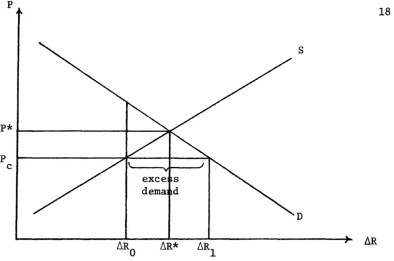
In the field market for natural gas, proved reserves are incremented through the discovery process and depleted through production. The amount of additions to reserves is positively related to some extent to the field price of gas contracts being signed at the locations close to where that volume of new reserves is available. The demands for new reserves by
pipe-lines could be specified in terms of field prices, but under conditions of shortage, the regulated ceiling price P prevails rather than the market demand price P*. This is illustrated in Figure 1. Under conditions of shortage, the quantity data fall on the supply but not on the demand func-tion, with the result that the demand function is not observable. At the same time, production out of reserves is affected by the reserve shortage. The supply curve for gas production consists of a marginal development cost curve which represents the cost of incrementing gas production (by running existing gas development wells at higher capacity or by drilling new development wells). The demands for gas production consist of the schedule of wholesale consumption draughts on the pipeline systems at prices equal to field prices plus the pipeline markups necessary to get the gas from the wellhead to wholesale buyers. These final demands may still be met at the beginning of the reserve shortage, as a result of the pipelines calling on existing reserves to produce at a higher rate.
Sufficient production under a condition of reserve depletion cannot be had indefinitely. Eventually, the amount of reserves available to back
production is reduced, and supply of production at ceiling prices is re-duced. As the reserve backing becomes smaller, marginal development costs will increase, so that in the presence of fixed ceiling prices, production will tend to fall and a gap is opened between the demands for production and the supplies that will be made available.
The marginal cost curves, the price markup, and a wholesale demand curve for new contracts, are all shown in Figure 2. In this diagram, the ceiling price is sufficient to bring forth production Q* which clears the market at wholesale price P*, which is just the field price plus the pipeline's markup. Under these conditions, the demand curve for produc-tion is "registered in the market" or observable as a total quantity
demanded with specific price level. However, if the regulated field price is reduced to a level P', excess demand will result equal to (Q1-Q0). The supply of production is reduced by price disincentives to a level below the demands put on the pipeline system by retail gas utility companies
serving final residential, industrial and commercial consumers. There are shortages both in field reserve and final production markets.
How would an increase in the ceiling price feed through these markets so as to reduce the production shortage? Consider, for example, an increase in wellhead ceiling prices under Federal Power Commission regulation. When the ceiling price is increased, the production cost curve remains fixed ini-tially, since reserve levels would not change immediately and therefore marginal production costs would not change. The higher price, however, would eventually elicit more production out of given reserves Q' and also reduce demands for production from Q1 to Q (as shown in Figure 3). Thus,
p*
P
C
Figure 1: Supply and Demand for Additional Reserves
¢/Mcf Mr . __ -- ..
qO qW Q1
Figure 2: Supply and Demand for Production
AR P*= P + C p'+ c
Q
¢/Mcf S z e Figure 3 p p D Qo Q1 (
QO
even within the short run, excess demand would be decreased by a price change from (Ql-QO) to (Qi-Q) even though the change may not be substan-tial because the "roll-in" pricing practices of the Commission would dampen the demand effect.
After two or three years, however, it is likely that reserve levels will have been increased as a result of the higher level of new contract prices. Higher ceiling prices would stimulate more exploratory drilling which, in turn, should result in new discoveries of gas that add to reserve
levels. At that point in time, a given level of production could be induced at lower marginal development costs because of the presence of higher reserve
levels. The supply of production curve would have shifted to the right. Even if demand were to remain at Q;, an increase in supply to Q would re-duce the extent of the shortage. After a few more years, the full effects of the ceiling price increase would have occurred, with the supply of pro-duction shifting further to the right so that excess demand had fallen to the even lower level of (Q-Q"')l
Of course, if we could increase the ceiling price just the right amount, accounting for resulting future shifts in the supply curve and independent shifts in the demand curve (resulting from increased population, national income, etc. as shown by D1 9 7 7), we might reach a situation where there was no excess demand in 1977. This is shown in Figure 4. Note, however, that until 1977, there will still be some amount of excess demand -- in the first
1
This analysis assumes that the pipeline markup is constant with respect to the level of production and that the difference between (P + price markup) and (P' + price markup) is equivalent to the "roll-in" price increase allowed under regulation. The econometric model discussed later deals with these matters of detail in specific price markup equations.
¢/Mcf
Q; Q* Q1
Figure 4
Qo
year after the price increase, for example, excess demand will be (Q1-Q0); not until 1977, when the supply curve, demand curve, and price line all
intersect at the same point, would there be a level of production, Q*, that results in no excess demand.
What if the field price of all gas were immediately and completely deregulated? This would result in a wholesale price increase to the level P* which, when the regulated markup is added on, would clear the production market immediately (as shown in Figure 5; the supplies and demands for pro-duction are both equal in one year to Q*). This substantial price increase would not be the end of the story, however. After three or four years, the supply curve will have shifted to the right, again because increased explo-ration and discoveries in response to the price increase would have added substantially to the reserve base. The demand curve would perhaps also
have shifted to the right after three or four years, but the net result would probably be a decrease in price and further increase in quantity of produc-tion over the four year period. This is illustrated in Figure 5 where the 1973 equilibrium quantity Q* is increased over time to Q** as the equilibrium field price P* falls to P**
f f
These examples indicate that pricing policies have a three or four step effect upon the size of the shortage, and it may take several years before the full effects of a price change become apparent. The econometric model presented in the next section allows us to analyze the dynamic impact of alternative price ceiling changes quantitatively.
¢/Mcf S1973 S1977 D1 97 Figure 5 .up
Q
lp qo q q---- ql3. An Econometric Model for Policy Analysis
Most previous econometric studies of natural gas have investigated either demand or supply of gas, but have neglected the simultaneous inter-action of these two sides of markets. Balestra, for example, in his
classic study of the demand for natural gas by residential and commercial consumers, assumed a perfectly elastic supply curve for production. This assumption was probably justified during the 1950's and 1960's since pro-duction of gas for final consumers took place on an "as needed" basis from large stocks of reserves, but it would not continue to be valid during the 1970's, however, as total gas demand exceeds the constraints on production imposed by smaller reserve levels. The supply studies of Erickson and Spann, and Khazzoom, similarly, are admirable attempts at defining and testing some of the relationships that exist in the gas industry, particu-larly those accounting for reduced reserve levels under price controls. But, to the extent that policies are changed in the future so that markets clear, and demand is once again observed, models of only the supply side of
markets will be inadequate to represent the effects of policy. If the industry is to be properly understood, then, production and reserve supply levels of the industry have to be analyzed as a simultaneous system.
The model developed as part of this study consists of a set of simul-taneous econometric relationships among several policy-related variables. Variables endogenous to the field market include, on the supply side, non-associated and (oil) non-associated discoveries of gas reserves, extensions and revisions of associated and non-associated reserves, and wells drilled.
These variables directly or indirectly depend on the field prices paid by pipelines in new contracts for gas. Field prices would be endogenous if demands could clear, but after ceiling prices were set by the F.P.C. in the 1960's, this variable became an exogenous policy variable.
Endogenous variables in the wholesale market include demand for pro-duction of gas and wholesale prices for three wholesale delivery sectors: mainline industrial sales, sales for resale that are ultimately industrial, and sales for resale that are ultimately residential and commercial.
Throughout the 1960's, wholesale production demand was completely satisfied even though there was excess demand for reserves (of course,
reserve-production ratios dropped dramatically during the decade) and thus wholesale demand equations can be estimated from data generated in this period.
An equation for marginal development costs (the "supply curve" for production in field markets), when combined with pipeline wholesale price markup equations, provide the wholesale supply curves for production. This allows us to determine "production out of reserves," as well as possible excess demand by comparing estimated "production out of reserves" with
estimated demands for reserves.
There is no single field market, nor is there a single wholesale market in the United States. Producers from around the country do not take their gas to the Chicago Board of Trade in order to make offers of sale to pipe-lines. Rather, there are several "regional" field markets and several "regional" wholesale markets, and the natural gas industry is characterized by the spatial interrelationships of these markets. This is taken into account by our econometric model. Field reserve and production equations are estimated for supply regions either separately or together with specific variables to account for the regionalization. Wholesale demand equations
are estimated for each of five parts of the country (each part roughly representing a regional market). Gas from each production district in the country is allocated to one or more wholesale consumption regions using the average allocation proportions that prevailed in the past
(based on the presumption that many new pipelines will not be built during the 1970's). In this way, excess demand can be computed on a region-by-region basis, as well as for the country as a whole.
3.1 Structure of the Model
The organization of the model is illustrated in Figure 6. Note, however, that this figure leaves out (for simplicity) the spatial inter-connections between production districts and regional wholesale markets. In the model as it actually runs, the wholesale prices of gas (for mainline sales and for sales for resale) are computed for each region of the country by taking the wellhead price of gas at the production source and adding a markup based on pipeline mileage and volumetric capacity. When a wholesale consumption region is supplied by more than one production district (as is usually the case), wellhead prices, mileages, and capacities are weighted according to previous actual proportions of production from each district. Let us now look at the individual parts of the model in more detail.
A. The Field Market
Probably the sector of the natural gas industry most difficult to capture in a conceptual model is the supply of new reserves. Most of the current controversy over regulatory policy centers on this sector -- whether or not reserve additions have been too low as a result of past regulatory
I-Z4 I ¢~ 0 I 4CH I WI 4 I ;I I 0X I H F-4 I t i U Q4 UU W -En I X 1: U c '0u I W :4 CYW l En C ag _ Q . > f ,o L I
4,
1-4 H lp(i En H U)> W cC ¢P4-4Po) 0z II W P4 l U) H 1 W Cl) H U) LQ.4'.
H q I:~ 0 , U) I '4Q~~~~~~~~Z · I Qp4~~l~~
Q~~~~~~~P I H-H Hz
H aI 44 " U14i P4~~ v~~ F1 27 1-1 '.4 H U) -_ P4P
Z; Pi
j 0 W P if H H Ct
P * P H E-z 0 H 1O H 9iE WW E--iW I E W CN l 1 'J
z
4 H pE-j PO 0 0 P4 0 Eq g4rXZ
00 H U-4 t ' P-,F
P4 14 P4 0 HU)zL I-- WES .4i
1 0 9d rz H . o) rlx W U H P4 P-Ii
P4 W H P4 d H U:) 0 P4 44 0 W P u 4 4WL I4 CD I P4 Hr ,C -4 C) U) 0z
z
0 H z E-1 H H I I E-t -xl4 H U) Nn I'l H H r-I 0 pq H I 1' 1U Ol l i I I-:4lP H -4 ^ I IZ~lH 0 I ¢I I H H^ z i I) H~pc p40 rz z z 1 0 9 l p I I , .g¢ > - -PQ I.4 0 IIIP-- 1*
R PX Iv v, II II c * a lP O l s~~~~~~~~~~~~~~~~~~~~~~_
_____
IIF_
· r s~~~~~~~~~~~~~~~~~~~
I BS i ....l
. !~ ~ ~
~
-__ t__2
W
-eI
l F 2 m PQ W IMI11IN
t'-Ri-policy. Actual additions to reserves through new discoveries are realized by a complicated process involving a large number of technological factors, and it may seem naive to try to model the process using a set of simple
econometric relationships. Structural equations can be formulated, however, that do link economic and technological variables that are important in gas reserve additions and also describe most simply and directly the regulatory
effects.
The major component of new reserve additions consists of new discoveries of both non-associated and associated gas (non-associated gas (N) is dry gas while associated gas (A) includes "dissolved" gas recovered from oil produc-tion, as well as "free" natural gas forming a cap in contact with crude oil). In our model, the discovery process begins with the drilling of wells, some of which will be successful in discovering gas, some will be successful in discovering oil (with associated gas), and some will be unsuccessful (i.e., dry holes). The drilling of wells depends largely on economic incentives; in our model, it is dependent upon past revenues from oil and gas production, average drilling costs, and a measure of drilling risk.
The model translates drilling activity into actual discoveries through two size-of-discovery variables, one for non-associated and one for asso-ciated gas. The size of discovery variable for non-assoasso-ciated gas, for example, gives for any district and any year the average number of Mcf of gas discovered per well drilled. The size of discovery variables themselves are explained partly by economic variables (e.g., oil and gas prices and drilling costs) but also by a depletion effect, in which extensive well
drilling in the past (measured by cumulative wells drilled) makes it more difficult to discover gas in the present.
Drilling may be divided into two basic modes of behavior, depending on whether it is done extensively or intensively. In extensive drilling, few wells are drilled, but those that are drilled usually go out beyond the
frontier of recent discoveries to open up new geographical locations or previously neglected deeper strata at old locations. Typically, this would
include drilling farther offshore, or onshore but at very great depth. Here the probability of discovering gas is rather small, but the size of discovery may be comparatively large. When drilling is done intensively, many small wells are drilled in an area that has already proven itself to be a source for gas discovery. Here the probability of discovering gas is larger, but the size of discovery is likely to be very small. In Figure 7,
typical probability distributions for discovery size are shown for each mode of drilling behavior. Relative to the intensive drilling mode, discovery size for extensive drilling has a larger expected value but also a larger variance.
The producer who is engaged in exploratory activity has, at any point in time, a choice as to whether any increases in his drilling activity will be extensive or intensive, and this choice will be influenced by changes (or expected changes) in economic variables. The actual influence of economic variables (field prices and drilling costs) will depend on the producer's geological portfolio (i.e., the set of regions over which he
Probability of Discovery intensive drilling extensive drilling , A/ Discovery Size on Initial Drilling
has drilling rights), as well as his own translation of present and past prices and costs into expectations on future prices and costs. Suppose, for example, that drilling costs decrease. As a result, a producer might decide to accept greater risk and drill on the extensive margin, with the result that average discovery size will (ex post) increase. On the other hand, the producer may own partially drilled reservoirs that now are worth drilling out. If this is the case, he might decide to drill on the inten-sive margin with a resulting ex post decrease in average discovery size. Thus it is not possible a priori to determine whether the effect of a decrease in drilling costs on average discovery size will be positive or negative. The same is true for a change in the price of gas.
Higher gas prices should indeed result in more drilling, but we would expect that over the years success ratios and size of finds will decrease as our finite resource stock begins to get depleted. One may model the exploration and discovery process stochastically as sampling with-out replacement, so that the expected value of discovery size would decrease as the sampling process went on. It is not our objective to try and pre-dict how big the total stock of gas yet to be discovered is, but we would like to embody a "depletion effect" in our model, at least to the point of being able to extrapolate the long-run decreasing returns to industry size that
See G. Kaufman, "Sampling without Replacement and Proportional to Random Size," Memorandum II, March 19, 1973.
2Industry spokesmen have claimed that higher gas prices result not only in more drilling activity, but also a shift to the extensive mode resulting in
larger discovery size. While we would expect higher gas prices to elicit more drilling, it is not clear that the additional drilling will be more
extensive. Our results do show a positive relationship between price and discovery size, but with a low elasticity.
have occurred over the past decade. We do this by including cumulative wells drilled as an explanatory variable in our "size of discovery" equations. If
the level of drilling activity is the same next year as it is this year, we would expect to see the level of new discoveries drop somewhat, and this is what would indeed happen if discovery size depends negatively on cumulative wells drilled.
Additions to gas reserves can also occur as a result of extensions and revisions of existing fields and pools. Extensions and revisions should also be expected to depend on price incentives, past discoveries of gas, existing reserve levels, and the cumulative effect of past drilling. Extensions are somewhat easier to model than revisions, and actually turn out to be influenced by price incentives, prior discoveries, and the total level of drilling acti-vity.l Revisions of established reserve levels are often erratic and difficult to predict. There is some effect from the price of oil relative to gas, but otherwise revisions will simply turn out to be proportional to prior disco-veries and reserve levels.
New discoveries, (DN, DA), extensions (XN, XA) and revisions (RN, RA) are combined to form additions to reserves. Aside from losses (L) and changes in underground storage (AUS), which we model as a constant
percen-tage of production, the only major subtraction from reserves occurs as a result of production (Q). Thus, for any time t, in a production district j, total gas reserves are given by the identity:
Rt,j = Rtl j + DNt,j + XNt j + RNt + DA + XA + RA
tj t-l,j t,j t,j tj tj tj t,j
- Q t,j t,j - AUSt,j
We see that the supply of new reserves is determined by adding new discoveries, extensions and revisions together and subtracting production
1
Extensions can result from either exploratory or development well drilling. Our model does not explain development well drilling, and therefore only exploratory wells are used to explain extensions.
(and also, of course, adjusting for losses and changes in underground storage). If the wellhead price of gas were not regulated, or if regula-tion were ineffective, then the demand for new reserves could be given by an equation for pipeline offers to buy reserve commitments at specified new contract wellhead prices. Since 1962, however, there has been excess demand for new reserves and thus the demand function for new reserves has not been observable. Instead, the price has been given by the exogenous ceiling price.
B. Production Out of Reserves
The supply of production as a function of price is just the marginal cost (in the short term) of developing existing reserves (e.g., drilling development wells and then operating them) to the point of actual gas production. Clearly, marginal production costs will depend on reserve levels relative to production, and as the reserve-to-production ratio becomes small, we would expect marginal costs to rise sharply.
Let us examine what marginal costs would be corresponding to a pro-duction level q out of proved reserves R. Assuming a constant decline rate, a, in percent per year,
a = q/R = /Reserve-Production ratio , (2)
we can write the proved reserve level as R = q f e tdt = q/a .(3)
Then for a discount rate 6 the "present-Mcf-equivalent" (PME) of a constant production level q is:
lOur thanks to M. Adelman and M. Baughman for their assistance on this part of the model.
PME = q 0f e(a+)t dt = q/(a+6) (4)
Now we assume that the development investment, I, needed to obtain the production level q is given by:
I = A + ce aq (5)
where A is a start-up cost, c is constant over the range of zero well inter-ference, and is a parameter with value around 10. Thus, when a is small
(e.g., the reserve-production ratio is larger than 10), I will be roughly linear in q, but when a becomes larger (e.g., the reserve-production ratio approaches 5), an exponential rise in costs begins to predominate. The marginal development cost (MDC) is then given by:
dI dI . dq d(PME) dq d(PME)
DI da + I dq (6)
(a dq aq d(PME)
MDC = ( eaq + cea) (a+6) 2
~a (a+6)2
= (a + l)ce 6 2
= (a + l)cS6ea (1+ . (7)
This marginal cost curve is illustrated in Figure 8 for 6 = 0.1, 8 = 10, c = 10, and R = 0.2 trillion Mcf. For small values of a (i.e., large reserve-production ratios), the curve is predominantly quadratic, and when a becomes large, the curve begins to look more like an exponential.
We estimate a marginal cost curve (which, when price is set equal to marginal cost, becomes our supply curve for production out of reserves)
better fit to recent data, it is also in keeping with our goal of calculating excess demand for gas under conditions of declining reserve-production ratios.
MDC (¢)
q (billion Mcf)
10 20 30 40
Figure 8: Hypothetical Marginal Cost Curve
C. The Wholesale Market
The supply of production -- determined by what is essentially a marginal cost curve for production out of reserves -- has to be put against
demands for that production by companies providing gas to final consumers. The demands for production are approximated by curves fitted on a disaggregated basis, namely by wholesale demand equations for (1) gas sales for resale
(split into commercial-residential gas, and industrial gas on the basis of percentages distributed to these two groups for ultimate consumption),
(2) gas sales directly off the pipelines for consumption, and (3) intrastate sales by producers and pipelines to final consumers. The wholesale prices of gas (disaggregated into a "sales for resale" price and a "mainline sales" price) is computed by adding a markup to the field price based on (a) the mileage between the production district and the consuming region, and (b) the volumetric capacity-of the pipelines.
The demand equations follow a general formulation, in which the quantity demanded is dependent on wholesale price, the price of alternative fuels, and "market size" variables such as population, income, and investment that
determine the number of potential consumers. In all of the equations, the
dependent variable will be new demand, 6Q, rather than the level of total
demand. In the short run, as Balestra has shown for residential gas [2],
the level of total demand should be relatively price inelastic and would depend on stock variables that do not change much in time (e.g., the total stock of gas burning appliances for residential gas). New demand, however,
should respond to the price of gas and to the price of competing fuels
(decisions to buy new appliances, for example, are affected by fuel prices). The new demand for gas, 6Q, is made up of the increment in gas consumption AQ = Qt-Qt-l' and of replacement for continuation of old consumption. To
find replacement, total residential and commercial gas demand could be considered to be a function of the stock of gas burning appliances, A:
Qt = At
Qt t
where X is the (constant) utilization rate. Then, if r is the average rate at which the stock of appliances depreciated, the replacement demand for gas
includes rAt 1, and total new demand is
6Qt = AQ + rAt_l ' (9)
Now substituting (8) into (9) gives:
6Qt = AQt + rQt-l . (10)
Thus, new demand for gas is the sum of the incremental change in total gas consumption (AQt ) plus the demand resulting from the replacement of old appliances.
Our a priori assumption is that new demand depends on prices and total income (through purchases of new appliances), and that the level of total demand is itself a function of income and population. Thus, we have for residential and commercial demand:
6QSRCRt,k = f(PSRt,k PFt,kYt,kk'Yt,k 6Nt,k ) (11) where PSR is the sales-for-resale wholesale price, PF is a price index of
competing fuels, Y is disposable income, and N is population, all in region k, and
6Yt,k = AYt,k+ rYt-l,k (12)
and
6N A +rN 1(13)
t,k = Nt,k rNt-l,k(13)
1
Balestra [2] distinguishes between two depreciation rates, one for gas ap-pliances and the other for alternative fuel-burning apap-pliances, since life-times for appliances using alternative fuels may be different. He then estimates the two depreciation rates by estimating an equation of the form:
QSRCRt = a0 + aPSRt + a2ANt aN 1 + a3N t_ + a4A Y t + a 6QSRCRt_-. (14)
The model is closed by spatially interconnecting production districts with consuming regions. A flow network is constructed which, based on
rela-tive flows over the past few years, determines where each consuming region obtains its gas. Average wholesale prices (again both for sales for resale and mainline sales) can thus be computed for each consumption region in the
country, since mileages and volumetric capacities are then determined. Wholesale demand (by type) is then also computed for each region of the country. Wholesale demands can be summed to produce total demand for each region of the country, and since we know what the supply of production will be to each region of the country, we can determine excess demand.
3.2 Estimation of the Model
The model was estimated using pooled cross-section and time-series data. The time bounds of the regressions are different for different equations, partly as a result of data limitations but also because of structural change over time in the industry. Wholesale demand equations, for example, were
estimated using data only from 1967 to 1971, even though data was available from as far back as 1960, because it was felt that demand elasticities have
The depreciation rate for gas appliances is then given by (l-a6). (His
results, however, gave an estimated a6 that was always greater than 1, which
cannot be justified theoretically.) The all-fuel depreciation rate comes out of equation (14) as either the ratio a3/a2 or a5/a4. Thus, the equation
is over-identified, and the depreciation rate can be obtained only by esti-mating (14) subject to the constraint of a3/a2 = a5/a4. (The resulting
estimation problem is non-linear, but Balestra uses an iterative method suggested by Houthakker and Taylor [12] to obtain an estimated depreciation rate equal to 0.11.) Rather than attempting to estimate one or more depre-ciation rates, we will use a single rate assumed to be equal to 0.1, and use this for both industrial and for residential and commercial demand.
changed considerably during the 1960's partly as a result of new air pollution standards.l
Cross sections were also different for different equations. Field market equations were estimated by pooling data from all of 19 F.P.C.
pro-duction districts, while individual sales-for-resale wholesale demand equations were estimated over what were considered to be the proper re-gional wholesale markets, and thus each used data pooled from five to ten states. District breakdowns and time bounds are summarized for all equa-tions of the model in Table 1.
A. Statistical Results
The regression results described below were obtained using two-stage least squares whenever unlagged endogenous variables appeared on the right-hand side of an equation. All of the equations are linear in form, with the exception of the equation describing production out of reserves, which is logarithmic in the price term (thus marginal production costs are
an exponential function of production and reserves). t-statistics are shown in parentheses below each estimated coefficient. Also listed for each equation are the R, F-statistic, standard error of the equation, Durbin-Watson statistic, and the mean of the dependent variable. Note
that the Durbin-Watson has limited meaning, since error terms may be auto-correlated across time and/or across cross-sections, and these effects are not separated.
1A test of this hypothesis and a more detailed study of demand will appear in a future paper.
r-. rl r r-_ -. r- -0 I I I I I I 'O ' 0\ 0I' 0' 0' O- m -I cv- m O I 1-1 -4 -4 --I 'A --0 o 0O O Z ! 4-0C o0 ceI 0 0 -H I -H -4 -Hi 4J 0-Ho -0 0cn d o H -H 0 ^C O H 0 o 5 ^ O 0 '.CC0i H wri co C CU U -H O 0a 0 0 O 0 -I vH X O v-4 v- I ciC00 * ^, -N v ON H 0 wr to r3 0 d 0 .rq-H CC .-H Z "a 0 . OH A at coX 4-JZ XS X >4> o P-4-') Xt 0' C), d : -.-v 0 :35-4i a) 0 E P a) P-, P 0 o 03 r-I C0 0 -C) a 0 C --4 0 v I -i ,4 -OC) C) 0C a) LOce F-i 0 - C t4-i Ocw-0 kA 0rl P -4 X PL4 c) :3 )' -0 -O 5-4 ul P P P P4 P -E-4 co :I HB 0 0 0 00 r- N O . ,- 0-v-I -I --I v-- -4 I I I I I r- r- r- r .
'-v-I -I -1 I-D -I0
-5 rq aI --s 0 -H H -c -i C C C)
~bO
0 C) rc ., oj m ZU CP C a co 5-4ciC) r.Pc-~co
z 54 + C h Wi X C 5 i 0O 1-) C, u -I 4-0 0 - c c q- Cde - 0) I -H 4 I: 0 JJ 0 P I 0 z u r-H I-I a) ,n co cm 4-J 0 -H 0 0 td o C) 0 C CJ ,-4 c bCO 4-10 H CZ F:-c z 0 cJ 0 C) 0 -H z 0 - a -H 4-) 0 ^,. r 4 N -H -H -I ¢ 0 --I co 4-) C) 0 av o -H D C d 0 cor. -H -H 3 c r-4 0 nqco 00 -H C u 5-U .CC CCl 4) 0 0 Ca2 X d Er q 0 co 4 , o H: v-- I-C) a, Cd rt a CC d co -H4 C) co c0 0 ci OC) '4 ( E4 ,Ž4 C)H h 40 c's Cd -r 3 CC 5w4) tA O C P o o o c 0 l r 1t 00 *H co 0 CC + ·: .0 ' 0 OX 0+ Cd H + "I r 4Q -, 0 0 an a rdq I + C H -H Cw 0 : 0 . i C H cO · -,. t t 0 +) -,.tI t~ n 0 P d ,i < ,1 ~ Z-Q -, C - or 1 ^1.0 O I X X CC ,0 rl d .- -O 0 P4 0 o 0 4 H 0 C ) ^ 0 OH + o- . -- o H + C 0d 0 o o i x C0 ¢ 0 cd CO vI u3 <d ^Z > '.M v-I CiO -H M 4VJ : 4 (V UCO -r. ;0 rlC) r1 .-H0 cri C' 4-) coi C) 4J 0 cn 4) ce -rI En 0 59-C3 0 I O v--H CC C ')~
C nC, 0 ^ '.-H c ci 0l 0 rl v- X C C0 i C ) C l . q -rEi Xh 4-) co ce v4 C 4 tS d d 4- c iiC)P cH 0 O a)4- c 0~4 -Kc/20 a o E0 C) .-H H--CC 0 -H 4-J co ;J U -H 0 4-iCC m C) 0 4 CC v-I C) 0 a)o
C 4-t n~.i
4-10 4-I :3 0 C)I r:3 .H E-C I'd m Cd M 0 -H 4-i C C1) I 0 C u li: -C H 0 -ICC 4J (J .r.1-4 C, 4-to :3 0 .,{ 4-)C) 0 ,:)0 P I r rH -:¢ 'C) C) v--I 0 0 -H EO 4-) CC) -H ri) .HOne of the difficulties in constructing a model of this sort is that one must work under the constraints imposed by data limitations. Data for many variables is either difficult or else impossible to obtain, particularly for years prior to 1966. In addition, much of the data is extremely noisy. As a result, a good deal of compromise was often required in estimating equations between functional forms that are theoretically pleasing and those that lend themselves to the existing data. This should be kept in mind when interpreting the estimation results.
A.1 Field Market Equations
The field market portion of the model contains seven stochastic equations that explain total exploratory well drilling (WXT), non-associated and associated average discovery size (SIZEDN, SIZEDA), extensions (XN, XA), and revisions (RN, RA). Non-associated and associated new discoveries
(DN, DA) can be determined from the two identities:
DNt = SIZEDNt j WXTtj (15)
DAt,j = SIZEDAt j ' WXTt j (16)
and the supply of new reserves is then determined from the identity in equation (1).
Exploratory well drilling responds to three economic incentives, all of which are exogenous to the model. The first of these is total revenues
(deflated by a GNP price index), REVD, from sales of both oil and gas at the wellhead. Exploratory drilling may result in the discovery of either gas or oil, and so total revenues is used as an explanatory variable. Note that changes in the price of gas (or the price of oil) can affect drilling activity through this revenue variable.