A surface based approach for constant scallop height tool path generation

(1)

HAL Id: hal-01076666

https://hal.archives-ouvertes.fr/hal-01076666

Submitted on 22 Oct 2014

HAL is a multi-disciplinary open access archive for the deposit and dissemination of sci-entific research documents, whether they are pub-lished or not. The documents may come from teaching and research institutions in France or abroad, or from public or private research centers.

L’archive ouverte pluridisciplinaire HAL, est destinée au dépôt et à la diffusion de documents scientifiques de niveau recherche, publiés ou non, émanant des établissements d’enseignement et de recherche français ou étrangers, des laboratoires publics ou privés.

A surface based approach for constant scallop height

tool path generation

Christophe Tournier, Emmanuel Duc

To cite this version:

Christophe Tournier, Emmanuel Duc. A surface based approach for constant scallop height tool path generation. International Journal of Advanced Manufacturing Technology, Springer Verlag, 2002, 19 (5), pp.318-324. �10.1007/s001700200019�. �hal-01076666�

(2)

A surface based approach for constant scallop height

tool path generation

Christophe Tournier* (tournier@lurpa.ens-cachan.fr) Emmanuel Duc* (duc@lurpa.ens-cachan.fr)

* LURPA - Ecole Normale Supérieure de Cachan 61 avenue du Président Wilson

94235 Cachan Cedex France

Abstract:

The machining of sculptured surfaces like molds and dies in 3-axis milling relies on the chordal deviation, the scallop height parameter and the planning strategy. The choice of these parameters must ensure that manufacturing surfaces respect the geometrical specifications. The current strategies of machining primarily consist in driving the tool according to parallel planes which generates a tightening of the tool paths and over quality. The constant scallop height planning strategy has been developed to avoid this tightening. In this paper, we present a new method of constant scallop height tool path generation based on the concept of the machining surface. The concept of the machining surface is exposed and its use to generate constant scallop height tool paths. The approach is confronted with existing methods in terms of precision and in particular its aptitude to treat curvature discontinuities.

Key words:

3-axis milling, free-form surfaces, ball endmill, machining surface, tool path, scallop height

(3)

Symbols:

SM machining surface

SD design surface

SSh constant scallop height surface

R tool radius (mm)

Sh scallop height (mm)

Ci tool path

CLi,j point on the tool path

Ti scallop curve

Pi,j Point onto the scallop curve

CLi,j point on the tool path

Ni,j surface normal

ni,j pipe surface normal

ti,j tangent vector to Ti

(4)

Introduction

The machining of sculptured surfaces like molds and dies in 3 or 5-axis end milling requires the construction of successive tool paths and their juxtaposition according to a machining strategy. The machining strategy relies on the choice of a tool driving direc-tion and two discretizadirec-tion steps, the step length along the path or chordal deviadirec-tion (longitudinal step) and the cutter path interval or scallop height (transversal step). The tool path is then made of a discrete set of points representing the successive positions of the tool centre which will enable it to cover the surface. If the numerical control unit can read and interpret tool paths expressed in a polynomial, canonical, B-spline or Nurbs format, the tool path consists of curves respecting the chordal deviation criterion.

The choice of the chordal deviation and the scallop height parameters must lead to the realization of manufactured surfaces respecting the geometrical specifications of form deviation and surface roughness [1]. For a given part, the use of High Speed Milling (HSM) makes it possible to increase the number of tool paths, therefore to reduce the scallop height, without increasing machining time [2]. However, the current strategies of machining primarily consist in driving the tool according to parallel planes, which does not optimize the rate of material removal. Along a tool path, the variations of the normal orientation on the surface in the perpendicular plane to the tool path generate a tightening of the tool path in its totality. This tightening increases machining time and creates over machining in some areas (Figure 1).

In order to increase the quality and the speed of machining, we propose to exploit the constant scallop height planning strategy. This strategy generates uniform scallops on the surface and ensures a better coverage of the surface by tool path. The narrowing of successive paths obtained with other strategies can be removed.

(5)

In the literature, few articles deal with the generation of constant scallop height tool paths for 3-axis milling with ball endmill [3] [4] [5]. Furthermore these methods are quite similar. Tool paths are planned in the parametric space and the two first funda-mental forms are used to evaluate the surface properties at the considered point.

In this paper, we use a new method of constant scallop height tool path generation based on the concept of the machining surface [6][7]. The machining surface enables us to consider the tool path as a surface and not anymore as a set of points (linear interpolation) or a set of curves (polynomial interpolation). Every curve onto the machining surface is a potential tool path which machines the surface without collision. Given a machining surface, the tool path generation consists in choosing a set of curves belonging to the surface. The knowledge of this surface gives us more elements to precisely plan the relative position of these curves.

In the continuation of the article, the concept of the machining surface is presented. Following its use to generate constant scallop height tool paths. The approach is then confronted with the existing methods and in particular its aptitude to treat curvature discontinuities on the surface.

The concept of the machining surface

The concept of the machining surface has been developed to improve the quality of the machined surfaces by associating a surface representation to the tool paths. First of all, the qualitative profits come from the integration of the functional constraints of design in the construction of the machining surface so that the machined surface respects the design intent. From a tool path generation point of view, the improvements come from the continuous representation of the tool path, contrary to the conventional approaches where the tool path is a discrete representation.

(6)

General definition of the machining surface: the Machining Surface is a surface including all the information necessary for the driving of the tool, so that the envelope surface of the tool movement sweeping the MS gives the expected free-form [6].

Considering each tool geometry and for each type for machining (3 or 5-axis) in end-milling or in flank-end-milling, a specific definition of the machining surface is proposed [7]. In 3-axis end-milling, the definition of the machining surface corresponds to the definition of general offset surface. Since we use the ball endmill in this article, the machining surface is the traditional offset surface.

The tool path generation using offset surfaces has already been the object of nume-rous papers [8][9]. Among the problems encountered in the tool path generation using offset surfaces, the most constraining are the problems of loops or self intersections and of precision [10] [11]. The problem of loops comes when using a tool which radius is larger than the smallest concave curvature radius of the surface. In order to be free from loop problems, we will consider tools whose radius is smaller than the smallest concave radius of curvature of the surface to be machined. This appears coherent within the framework of finishing milling used to generate constant scallop height tool paths. The problem of precision comes from the model of representation of offset surfaces. Indeed for most cases, it is not possible to model these surfaces by a parameterized NURBS surface without approximations. Therefore we will adopt in our study an implicit repre-sentation of the machining surface: S_M(u,v)=S_D(u,v)+R⋅N(u,v)

The advantage to use the machining surface to generate tool paths with constant scallop height, is that the distance between the driven point (the tool center) and the associated point on the scallop curve is constant and equal to the radius of the tool. In the methods where the point of contact between the tool and the surface (CC point) is

(7)

driven, the distance between the CC point and the associated points of scallop varies all

along the tool path.

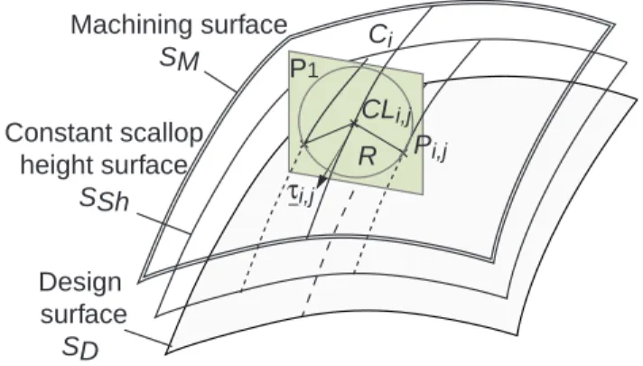
The geometry of constant scallop height tool path

Let us consider two adjacent tool paths Ci et Ci+1 located onto the machining surface

SM, offset surface of amplitude R of the design surface, and the surface of constant

scallop height SSh, offset surface of amplitude equal to the scallop height Sh. For each

path, the envelope surface of the tool movement is a pipe surface the radius of which is equal to the tool radius and whose spine is the curve followed by the tool center. The scallop curve generated by the two paths is thus the intersection of the two pipe surfaces. In the case of a constant scallop height machining, this curve belongs to the surface of constant scallop height SSh.

Practically, the previous geometrical problem can be uncoupled in two successive problems. The first problem consists in finding the scallop curve Ti which is generated

by the first path Ci, where Ti is the intersection of the envelope surface associated to Ci,

with the surface of constant scallop height SSh (Figure 2). In the second problem, we

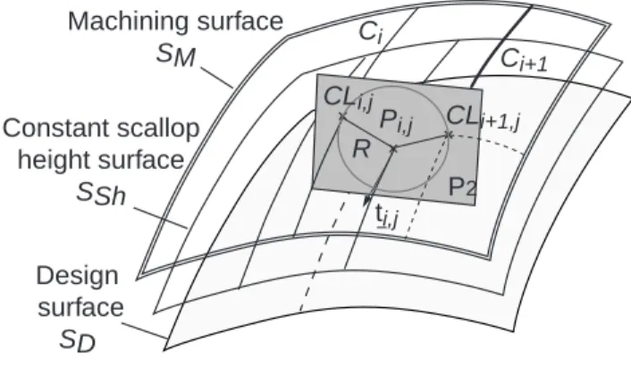
build the adjacent tool path Ci+1 which belongs to the machining surface SM starting

from the scallop curve, so that the scallop curve Ti is the intersection of the two pipe

surfaces associated to Ci and to Ci+1 (Figure 3).

We show now that the curve Ci+1 is the intersection of the machining surface with

the pipe surface generated by the scallop curve Ti .

For each point Pi,j onto the scallop curve Ti , the tangent ti,j to the curve Ti is given by

the cross product:

j 1, i j i, j i, =n ∧n + t ₍₁₎

(8)

with ni,j and ni+1,j the unit normals to the pipe surfaces at the considered point: j i, j 1, i j 1, i j i, j i, j i, =CL P n + =CL + P n ₍₂₎

CLi,j and CLi+1,j are the tool locations which generate the point Pi,j onto the scallop

curve.

To a scallop point Pi,j, we can associate a tool center point CLi+1,j on the path Ci+1

with: 0 R P) , dist(CL_i₊_1,_j = n_i₊_1,_j ⋅t_i,_j = ₍₃₎

The searched path Ci+1, locus of the points CLi+1,j, thus belongs to a pipe surface of

radius R whose spine is the scallop curve Ti. Finally, the tool path Ci+1 is the intersection

of the previous pipe surface and the machining surface SM. Moreover, one will notice

that the intersection of the pipe surface associated to Ti, with the machining surface SM

actually gives two curves which one is Ci+1 and the other is Ci, which is in agreement

with (1) and (2). The construction of constant scallop height tool paths can thus be carried out by successive intersections between pipe surfaces and the machining and constant scallop height surfaces.

The methods developed by Suresh and Yang [3], Sarma and Dutta [4], and Lin and Koren [5] have in common the planning of tool paths in the parametric space while using fundamental forms to define differentials characteristics of the surface at the considered point. The initial path is sampled to calculate the points of the following path. This last one is then built by interpolation of calculated points. To be able to compare performances of our approach with existing methods and not to leave ambiguities on the way are generated the surface intersections, we suggest to generate successive tool paths point by point in the parametric space. The initial path is sampled

(9)

and in every point we compute the associated scallop point as well as the corresponding point of the next tool path.

The first part of the problem is the search for the point Pi,j element of the scallop

curve when the tool is located on the point CLi,j on the initial path. The point Pi,j is given

by: (Figure 4)

{ }

SSh

{

PlaneP1

} {

SphereS1

}

P = ∩ ∩ where Sphere S1 is the active part of the tool

and Plane P1 the plane normal to Ci passing through CLi,j.

The second part of the problem consists in determining the point CLi+1 of the

following path from the scallop point Pi,j. The point CLi+1,j is given by: (Figure 5)

{ }

SSh

{

PlaneP2

} {

SphereS2

}

1 i

CL = ∩ ∩

+ where Sphere S2 is the active part of the

tool and Plane P2 the plane normal to Ti passing through Pi,j.

Contrary to [3] and [5] where the assumption is made that the problem is plane, i.e. that the point CLi+1,j is located in the plane perpendicular to Ci passing through CLi,j,

construction is done in two different planes. The point Pi,j is in the P1 plane and the

point CLi+1,j in the P2 plane. Actually, the problem is indeed plane because the three

points Pi,j, CLi,j et CLi+1,j are in the P2 plane of normal ti,j (1)(2) but this plane is not

known at the beginning of the construction.

Algorithms

In existing methods, it is necessary to associate a curve with each whole of calculated points CL to generate the following path. This is necessary to calculate the tangent

vector to the tool path or to the scallop curve in order to define the study plane. This is not the case when using the method of the machining surface. The tangent vector is given by the cross product of the normals of both surfaces considered for intersection

(10)

calculation (1). In order to compare the methods, we thus propose to consider two versions of the method of the machining surface. We use the association of curves to compare the performances of the various methods (algorithm 1) and the other does not in order to study the impact of curve association on the behaviour of calculated paths (algorithm 2).

Algorithm 1: Computation of the tool positions CLi,j on successive path Ci with association of curve

Initial conditions: Design Surface SD : S(u,v)

Constant Scallop height Surface SSh : S(u,v)+Sh . n(u,v) Machining Surface SM : S(u,v) + R . n(u,v)

For i = 1,n For j = 1,m

Compute cutting plane P1j, perpendicular to Ci at CLi,j Compute the intersection point Pi,j of SSh, P1j and Sphere S1 End

Associate the scallop curve Ti to {Pi,j} For j = 1,m

Compute cutting plane P2j, normal to Ti at Pi,j

Compute the intersection point CLi+1,j of SM, P2j and Sphere S2 end

Associate the tool path Ci+1 to {CLi+1,j} End

Algorithm 2 : Computation of the tool positions CLi,j on successive path Ci without association of curve

Initial conditions : Design Surface SD : S(u,v)

Constant Scallop height Surface SSh : S(u,v) + Sh . n(u,v) Machining Surface SM : S(u,v) + R . n(u,v)

For i = 1,n For j = 1,m

Compute the tangent to the intersection curve between the pipe surface (Ci) and SSh Compute the intersection point Pi,j of SSh, P1j and Sphere S1

End For j = 1,m

Compute the tangent to the intersection curve between the pipe surface (Ti) and SM Compute the intersection point CLi+1,j of SM, P2j and Sphere S2

End End

The selected method for curve fitting is the interpolation by cubic B-spline curves. We use a parameter setting proportional to the chord length [12]. Whatever the method, tool paths are calculated in the parametric space. In the case of algorithm 1, it is necessary to calculate the tangent to the current curve (scallop curve or tool path) so that

(11)

the cutting plane (P1 or P2) is defined. The tangent vector t to a curve C(t) or C(u(t),v(t))

lying on the surface Φ(u,v) = S(u,v) + d . N(u,v) where d takes the value R or Sh is

given by : v u v(t) Φ Φ (t) u ⋅ + ⋅ = & & t ₍₄₎

where u&(t)and v&(t)⋅are the parametric tangent vectors and Φ and _u Φ the partial _v derivatives of the surface given by:

α N d α S α Φ ∂ ∂ ⋅ + = (5) α N ∂

∂ _{is the curvature operator defined by:}

β β α − = ∂ ∂ _b _S α N (6) Finally, )) S b S (b d (S (t) v )) S b S (b d (S (t) u t = & ⋅ _u− ⋅ ₁1⋅ _u+ ₁2⋅ _v + & ⋅ _v − ⋅ 1₂⋅ _u+ ₂2⋅ _v (7) b is the tensor of curvature or the second fundamental form.

Algorithms behaviour

At first, the methods are applied on a Nurbs surface delimited by two lines and two arcs of circle (Figure 6). It thus presents concave and convex areas and does not include any discontinuity of tangency or of curvature. The tool radius R is 10 mm and the speci-fied scallop height is 0.001 mm.

The initial tool path is an isoparametric curve of the surface. Then, the initial tool path is sampled in points and points of the adjacent path are built one by one to define a first path and so on until the last tool path. Throughout this process we observe the propagation of the initial points, it is the traceability. We can thus visualise the tool

(12)

center location or the surface contact point calculated before curves associations. Indeed, the interpolation hides the behaviour of each algorithm.

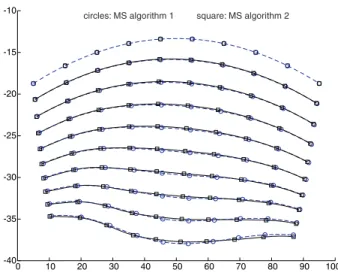
The first test consists in comparing the proposed method with the method suggested in [3] and [4]. We pointed out that these methods use the association of curves inevitably. We thus use the method of the machining surface with association of curve (algorithm 1). The selected initial tool path is the isoparametric curve v0 = 1/3, and the

machining is done in the -y axis direction (Figure 7). The tool paths are represented by curves with the points used for computation. The progression is done from the top to the bottom and only one tool path on ten is represented for more clearness. We notice first of all that the three curves diverge progressively with machining. Curves generated by Suresh & Yang [3] are those which present the greatest variation in comparison to the others. In their approach, the problem is regarded as plane and one passes from one path to the other without passing by the scallop curve (what makes it the fastest method). Moreover, the distance between successive tool paths is calculated in an approximate way. The two other methods are relatively close despite of a slight divergence.

The second test consists in studying the influence of curve association on the calcu-lated tool paths (Figure 8). The two versions of our method are compared. It is noticed that the interpolation largely influences the results. Although tool paths are very similar, points position calculated with both methods vary. This is explained by the fact that the interpolation modifies the direction of the tangent vector to the curves at the calculated points, but does not modify the distance between two adjacent tool positions. Adjacent points are not evaluated in the correct direction. We could have introduce tangency constraints in the interpolation scheme but it wouldn’t have been representative of the possibilities offered by the other methods.

(13)

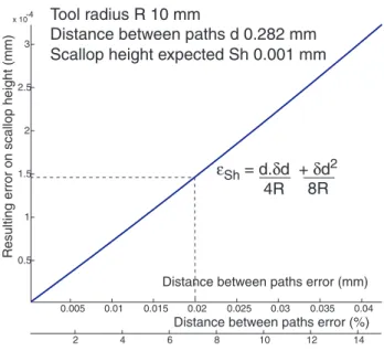
Moreover, differences between tool paths are found on the resulting scallop height. Let us take the example of the difference between the tool paths generated by the method [3] and those generated with the method of the machining surface without association of curve (Figure 7). At the end of 100 tool paths, the distance between the ways is approximately 2 mm. If one considers that the drift is constant progressively with the construction of the tool paths, it represents approximately 20 µm (7%) of error between two consecutive tool paths, that is to say an error on the scallop height of 0,15 µm (15%) (Figure 9).

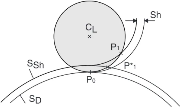
Behaviour on curvature discontinuities

We study in this part the treatment of curvature discontinuities. Indeed, the existing methods make the assumption that the surface curvature is constant around the consi-dered point. This is not a problem during the machining of a B-spline surface made up of only one patch because this type of surface garantee the curvature continuity. But the majority of industrial parts are modelled with a multitude of patches connected in tangency and eventually with NURBS surfaces presenting curvature discontinuities. For example it is the case when we introduce blending radii. Let us consider the machining of a cylindrical surface along its generatrices whose profile (Figure 10) presents a curvature discontinuity at the point P0. The considered point is in the convex part of

surface before P0 and with the hypothesis of constant curvature, the adjacent tool

location calculated is in P*1 and not in P1 as it should be. The resulting scallop height is

thus not the expected one.

We thus study the behaviour of our algorithm and those developed in [3] and [4]. We consider the machining of a sphere lying on a plane with a connection in tangency (Figure 11). The surface consists of three surfaces: a half sphere (radius 10 mm), a

(14)

portion of torus (radii 10 and 20 mm) and a plane. It presents two curvature discontinui-ties along the profile. The first one is located at the linking between the plane and the torus, the second between the torus and the sphere.

The adopted machining strategy is a machining according to the circular isoparame-tric from the outside of the surface towards the top of the sphere. Discontinuities are then well situated between two adjacent tool paths. We observe the scallop left by the tool at the two curvature discontinuities, with the three methods of tool path calculation. It is also pointed out that for a given scallop height and a given tool radius, the tool paths are more spaced (resp. less) when the curvature is concave (resp. convex).

To compare the methods, the scallops left by the tool are built with the method of the Z-buffer. We build in the zone of interest a network of lines parallel to the z axis and laid out on a grid whose step indicates the precision. The step of the square grid is set to 0.025 mm. Then, we carry out the intersections between this network of lines and the envelope surfaces of the tool movement.

Results (Figure 12) show that methods that rely on constant curvature generate an abnormal scallop on the discontinuity, which is not the case for the method of the machining surface. At the junction between the torus and the sphere, results show a higher scallop than the others with the passage of discontinuity. The distance between paths is calculated as if the curvature were concave (torus) whereas it is convex (sphere). With a constant distance between path, the scallop height is larger on the sphere than on the torus. Between the planar zone and the torus, the scallops in errors are smaller. The algorithms calculate a distance between path as if the curvature were null (plane) whereas it is concave (torus). With a constant distance between paths, the scallop height is lower on the torus than on the plane.

(15)

The experimental results confirm our assumptions on the influence of the curvature approximations. Approaching a surface by its osculating sphere during the calculation of constant scallop height tool path does not allow the correct treatment of curvature discontinuities. Thus molds and dies containing many blending radii cannot be machined with such algorithms, plastic injected molds in particular. The method of the machining surface successfully the treats curvature discontinuities by leaving a scallop in accordance with the specifications.

Conclusion

The concept of the machining surface enables to adopt a new method to generate constant scallop height tool path which shows benefits. First of all, there is no needs to associate an interpolating curve to build consecutive tool paths. Without interpolation, the proposed method is more accurate than the other methods. It doesn’t accumulate error from the beginning of the tool path calculation. Moreover, the method is characte-rized by its aptitude to treat curvature discontinuities. However, it should be noticed that these improvements increase computation time.

The concept of the machining surface also offers a framework to generate constant scallop height tool paths with flat-end or filleted endmills in 3-axis milling. But, whatever the method or the tool employed, it becomes necessary to tackle the problem of the tool path planning. Indeed, according to the initial tool path and the topology of the design surface, we have to extrapolate the tool paths close to the borders of the surface. Furthermore, the constant scallop height tool paths might contain loops. These loops could be eliminated but some tangent discontinuities would appear on the tool path.

(16)

References

[1] C. Lartigue, E. Duc, C. Tournier, Machining of free-form surfaces and geometrical specifications, IMechE Journal of Engineering Manufacture, vol. 213, pp.21-27, 1999.

[2] H. Schulz, S. Hock, High-speed milling of dies and moulds, cutting conditions and technology, Annals of the CIRP, 44/1, pp.35-38, 1995.

[3] K. Suresh, D.C.H. Yang, Constant scallop-height machining of free-form surfaces, Journal of Engineering for Industry, vol. 116, May 1994.

[4] R. Sarma, D. Dutta, The Geometry and Generation of NC Tool Paths, Journal of Mechanical Design, vol. 119, 1997.

[5] R-S. Lin, Y. Koren, Efficient tool-path planning for machining free-form surfaces Journal of Engineering for Industry, vol. 118, February 1996.

[6] E. Duc, Usinage des formes gauches, contribution à l'amélioration de la qualité des trajectoires d'usinage, Thèse de Doctorat ENS Cachan, 1998.

[7] E. Duc, C. Lartigue, C. Tournier, P. Bourdet, A new concept for the design and the manufacturing of free-form surfaces: the machining surface, Annals of the CIRP, vol. 48/1, pp. 103-106, 1999.

[8] K.I. Kim, K. Kim, A new machine strategy for sculptured surfaces using offset surface, International Journal of Production Research, vol. 33, no 6, 1995.

[9] K. Tang, C.C. Cheng, Y. Dayan, Offsetting surface boundaries and 3-axis gouge free surface machining, Computer Aided Design, vol. 27, no 12, pp. 915-927, 1995. [10] R.T. Farouki, The approximation of non-degenerate offset surfaces,

Computer Aided Geometric Design, vol. 3, pp.15-43, 1986

[11] T. Maekawa, W. Cho, N.M. Patrikalakis, Computation of self intersections of offsets of Bezier Surface Patches, Journal of Mechanical Design, vol. 119, June 1997.

(17)

D D n n D Sh Distance between paths on part ~D Direction of machining d Distance between paths on plane Over Machining

(18)

Ci Machining surface SM Constant scallop height surface SSh Design surface SD Ti R ni,j Pi,j CLi,j Ni,j Pipe surface ti,j

(19)