HAL Id: hal-02357025
https://hal.archives-ouvertes.fr/hal-02357025
Submitted on 9 Nov 2019
HAL is a multi-disciplinary open access
archive for the deposit and dissemination of
sci-entific research documents, whether they are
pub-lished or not. The documents may come from
L’archive ouverte pluridisciplinaire HAL, est
destinée au dépôt et à la diffusion de documents
scientifiques de niveau recherche, publiés ou non,
émanant des établissements d’enseignement et de
Par Means Parallel: Multiplicative Linear Logic Proofs
as Concurrent Functional Programs
Federico Aschieri, Francesco Genco
To cite this version:
Federico Aschieri, Francesco Genco. Par Means Parallel: Multiplicative Linear Logic Proofs as
Con-current Functional Programs. POPL 2020, Jan 2020, New Orleans, Louisiana, United States.
�hal-02357025�
Par Means Parallel: Multiplicative Linear Logic
Proofs as Concurrent Functional Programs
Federico Aschieri
∗and Francesco A. Genco
†November 8, 2019
Abstract
Along the lines of Abramsky’s “Proofs-as-Processes” program, we present an interpretation of multiplicative linear logic as typing system for concur-rent functional programming. In particular, we study a linear multiple-conclusion natural deduction system and show it is isomorphic to a simple and natural extension of λ-calculus with parallelism and communication primitives, called λ`. We shall prove that λ` satisfies all the desirable properties for a typed programming language: subject reduction, progress, strong normalization and confluence.
1
Introduction
The Proofs-as-Processes Program
Introduced by Girard in 1987, linear logic was announced right off the bat as the logic of parallelism. According to [17], the “connectives of linear logic have an obvious meaning in terms of parallel computation (...) In particular, the multi-plicative fragment can be seen as a system of communication without problems of synchronization.” Stimulated by this remark and the further observation that “cut elimination is parallel communication between processes” ([18], pp. 155), Abramsky [1] launched the “Proofs-as-Processes” program, whose goal was to support with computational evidence Girard’s claims. Namely, the goal was “to show how a process calculus, sufficiently expressive to allow a reasonable range of concurrent programming examples to be handled, could be exhibited as the computational correlate of a proof system” [1]. A candidate process calculus was Milner’s π-calculus [28]; a possible proof system, the linear sequent calculus. The hope was that linear logic could provide a canonical and firm foundation to concurrent computation, serving as a tool for typing and reasoning about communicating processes.
∗Funded by FWF project P32080-N31.
Early Successes and Limitations
After early works of [8] and [7], the turning point was the discovery by Caires and Pfenning [10] of a tight correspondence between intuitionistic linear logic and a session typed π-calculus, the motto being: linear propositions as session types, proofs as processes, cut-elimination as communication. This was yet another instance of the famous Curry-Howard correspondence [38], linking proofs to programs, propositions to types, proof normalization to computation. Soon after, Wadler [37] introduced the session typed π-calculus CP, shown to tightly correspond to classical linear logic.
This important research notwithstanding, it appears that there is still ground to cover toward canonical and firm foundations for concurrent computation. First of all, asynchronous communication does not appear to rest on solid foun-dations. Yet this communication style is easier to implement and more practical than the purely synchronous paradigm, so it is widespread and asynchronous typed process calculi have been already investigated (see [16]). Unfortunately, linear logic has not so far provided via Curry-Howard a logical account of asyn-chronous communication. The reason is that there is a glaring discrepancy between full cut-elimination in sequent calculus and π-calculus reduction which has not so far been addressed. On one hand, as we shall see, linear logic does support asynchronous communication, but only through the full process of cut-elimination, which indeed makes essential use of asynchronous communication. On the other hand, the π-calculus of [10] only mimics a partial cut-elimination process that only eliminates top-level cuts. Indeed, by comparison with its type system, the π-calculus lacks some necessary computational reduction rules. Some of the missing reductions, corresponding to commuting conversions, were provided in Wadler’s CP. The congruence rules that allow the extra reductions to mirror full cut-elimination, however, were rejected: in Wadler’s [37] own words, “such rules do not correspond well to our notion of computation on processes, so we omit them”. A set of reductions similar to that rejected by Wadler is regarded in [32] as sound relatively to a notion of “typed context bisimilarity”. The notion, however, only ensures that two “bisimilar” processes have the same input/output behaviour along their main communication channel; the inter-nal synchronization among the parallel components of the two processes is not captured and may differ significantly. Thus, the extensional flavor of the bisim-ilarity notion prevents it from detecting the intensionally different behaviour of the related processes, that is, how differently they communicate and compute.
Attempts to model asynchronous communication by mirroring full cut-elimination with Milner’s π-calculus are indeed bound to fail. An example will clarify the matter. In the process νz(x(y).z(w).P | z[a].Q), the second process z[a].Q wishes to transmit the message a along the channel z to the first process. How-ever, the first process is not ready to receive on z yet: it is designed to first receive a message on the channel x. In Milner’s π-calculus, this is a deadlock, because input and output actions are rigidly ordered and blocking, for the sake of synchronization. Indeed, as the heir of CCS [26], π-calculus was born as for-malism for representing synchronization: a communication happens when two
processes synchronize by consuming two dual constructs, as for instance x m and x(y). However, when a process is seen as a proof in the logical system, the order between prefixes becomes less relevant, thus in CP there is an extra commuting conversion
νz(x(y).z(w).P | z[a].Q) 7→ x(y).νz(z(w).P | z[a].Q)
In CP, there is no further reduction allowed, and rightly so: otherwise the blocking nature of the prefix x(y) would be violated, making the very construct pointless for synchronization. On the other hand, for cut-elimination the now possible reduction
x(y).νz(z(w).P | z[a].Q) 7→ x(y).νz(P [a/w] | Q)
is needed. In this case, however, as we have seen the very existence of a con-struct for input becomes misleading and it would be more coherent to drop it altogether, so that the first process would be directly re-written and reduced as follows
νz(P | w[a].Q) 7→ νz(P [a/w] | Q)
This is indeed the approach of the present paper. Sensitive to similar concerns, [21] introduced HCP, which features delayed input-output actions, modeling a form of asynchrony. However, the change in the transitions with respect to CP undermines the synchronous nature of Milner’s π-calculus, as we have seen, making HCP quite a different calculus and questioning its canonicality. Moreover, HCP comes at the cost of adding more structure, in the form of the hypersequent separator [6], to the linear sequent calculus. In HCP this structure is logically redundant, whereas Avron employed it to increase the logical power of sequents. On the other hand, the added structure enables HCP to enjoy a nice isomorphism with proofs.
There are other limitations in the current linear logic foundations of concur-rent computation. The linear sequent calculus fails to combine seamlessly func-tional and concurrent computation. Indeed, according to Abramsky et al. [2] it is a “major open problem (...) to combine our understanding of the functional and concurrent paradigms, with their associated mathematical underpinnings, in a single unified theory”. The sequent calculus falls short in several other respects: it prevents deadlocks, but by excessively restricting possible commu-nication patterns, for instance by forbidding cyclic configurations; it does not permit in any simple way code mobility, that is, the ability to communicate code, like in higher-order π-calculus [35]; it does not represent multi-party com-munication sessions; its syntax does not match exactly the syntax of processes. In order to address some of these pitfalls, much work has been done, by ei-ther considering non-standard proof systems for linear logic or by extending the logic itself; unfortunately for the canonical-foundation enterprise and prac-tical usability, these systems tends to be proof-theoreprac-tically artificial. A system adding a functional language on top of linear-logic-based typed π-calculus was studied in [36]. A solution for allowing, also in the context of the session typed
π-calculus, cyclic communication patterns, was given in [13] by coming up with a new variant of linear logic; this makes it possible, for example, to imple-ment Milner’s scheduler process. Multi-party session types have been treated for example in [11]. A hypersequent proof system for linear logic whose syntax perfectly matches the syntax of π-calculus has been introduced in [21]. A logic for typing asynchronous communication in a non-standard process calculus has been proposed in [34].
λ
`: A Concurrent Extension of λ-Calculus Arising from
Linear Logic
We shall illustrate a new approach in the study of linear logic as typing system for concurrent programs. Our framework does not suffer any of the mentioned limitations of linear sequent calculus. Inspired by [15, 29], we move away from sequent calculus and adopt a multiple-conclusion natural deduction for multi-plicative linear logic, which we show to be isomorphic to a concurrent extension of λ-calculus, called λ`. As a result, λ` is typed by linear multiple-conclusion natural deduction; it is naturally asynchronous, yet it can model synchronous communication as well; it allows arbitrary communication patterns, like cyclic ones, but prevents deadlocks; it allows higher-order communication and code mobility; it mirrors perfectly a full normalization procedure resulting in ana-lytic proofs; its types can be read as program specifications in the traditional way, although they do not describe communication protocols as session types do.
The typing system of λ`, in its non-linear variant, has been very well studied: computationally, it was famously interpreted by Parigot [30] as λµ-calculus; proof-theoretically, it was thoroughly investigated by [12]. Although proof-nets have sometimes been dubbed “the natural deduction of linear logic”, our typing system is closer to a natural deduction. It is not exactly natural deduction [33], since it is multiple-conclusion, hence it is natural for building and typing parallel programs, but not much so for modeling human deduction. However, our system is based on natural-deduction normalization rather than sequent-calculus cut-elimination and linear implication ( is a primitive connective, with the standard introduction and elimination rules. Like proof-nets (see [17], [19]), λ`abstracts away from those inessential permutations in the order of rules that plague multiple-conclusion logical systems. As a result, λ` avoids commuting conversions, which have never been convincing from the computational point of view. Actually, λ`is not only a concurrent λ-calculus, it also looks like a natural deduction version of proof nets. Finally, it enjoys all the good properties that a well-behaved functional programming language should have: subject reduction, progress, strong normalization, and confluence. It is a step forward in the direction of that elusive concurrent λ-calculus which Milner attempted to find, before creating CCS out of the failure1.
1According to Milner [27], “CCS is an attempt to provide a paradigm for concurrent
The Insight
The main insight behind the typing system of λ` is to break into two rules the linear implication introduction. One rule is intuitionistic and yields functional abstraction, the second is classical and yields communication. Namely, the first rule, taken from [15], introduces the λ-operator, the second a communication channel with continuation:
Γ, x : A ⇒ t : B, ∆
Γ ⇒ λx t : A ( B, ∆ ( I ( if x occurs in t)
Γ, x : A ⇒ t : B, ∆
Γ ⇒ x. t : A ( B, ∆ ( I ( if x occurs in ∆) Indeed, a communication channel x. t is supposed to take as argument a term
u : A, transmit it along the channel x and then continue with t : B. We shall indeed denote the application of x. t to u as xu.t, as in π-calculus: a promising sign!
The parallel operator | is introduced by the` introduction rule: Γ ⇒ s : A, t : B, ∆
Γ ⇒ s | t : A` B, ∆ `I
finally doing justice to the` connective, called par since the beginning.
2
Multiplicative Linear Logic as a Concurrent
Functional Calculus
In this section, we present the syntax, the typing system NMLL (Natural deduc-tion for Multiplicative Linear Logic) and the reducdeduc-tion rules of the concurrent functional calculus λ`.
2.1
The Calculus λ
`Definition 2.1 (Terms of λ`). The untyped terms of λ` are defined by the following grammar:
u, v ::= ◦ (terminated process) | x. u (output channel x with continuation) | x y u (output channels x, y without continuation) | u | v (parallel composition) | close(u) (process termination)
| x (variable)
| u v (function application) syntactic sugar
| λx u := x. u (function definition (provided x occurs in u)) | xv.u := (x. u)v
The calculus λ`is nothing but a linear lambda calculus extended with com-munication primitives. When x occurs in u, the operator x. u is denoted and behaves exactly as λx u. When x does not occur in u, the term x. u behaves as an output channel x followed by a continuation u. Channels in λ`are thus first-class citizens that can be transmitted, shared, moved and applied to messages just like functions to arguments. When the channel x. u is applied to an argu-ment v, it will be denoted as xv.u, because it behaves exactly as its π-calculus counterpart: it transmits the message v and continues with u. The term x y u transmits the two messages contained in u along the channels x and y and then terminates. Indeed, as it will be clear from the type system, the term u inside x y u must be of type A` B and must contain two messages: the term of type A and the term of type B.
If we omit parentheses, each term of λ` can be rewritten, not uniquely, as a parallel composition of several terms: t1 | t2 | . . . | tn. We will adopt this
notation throughout the paper since it is irrelevant how the parallel operator | associates.
Remark 2.1. An alternative choice for the syntax of λ` may have been:
u, v ::= x | u v | λx u | xv.u | u | v | x y u | ◦ | close(u) Then the operator xv.u would have been typed by a cut-rule and the construct x. u would have been defined as: λy xy.u. This approach would have raised some technical complications: when transmitting a message v, one would have to deal with the free variables of v which are bound by λ operators occurring outside v. A similar issue is solved in [4], and a simpler solution could be adopted here. Nevertheless, we adopt the present approach, as it is the smoother.
2.2
The Typing System NMLL
Definition 2.2 (Types). The types of NMLL are built in the usual way from propositional variables, ⊥ and the connectives ( and `.
Since the typing system of λ` is classical linear logic, the ⊗ connective can be defined in terms of the others. Indeed, its computational interpretation seems less primitive, as it defines no computational construct that is not already captured by ( and `. Hence, we leave it out of the system.
Definition 2.3 (Sequents). The judgments of the typing system NMLL for λ` are sequents Γ ⇒ ∆, where:
1. Γ = x1 : A1, . . . , xn : An is a sequence of distinct variable declarations,
each xi being a variable, Ai a type and xi6= xj for i 6= j.
2. ∆ = t1: B1, . . . , tn : Bn, tn+1, . . . , tm, each ti being a term of λ` and Bi
a type.
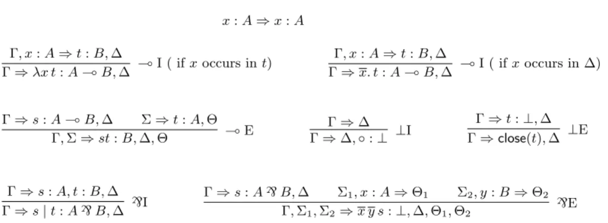
The typing system of λ` is a linear version of the multiple-conclusion classical natural deduction of [12]. It is presented in Table 1 and discussed in detail below. As usual, we interpret a derivable sequent Γ ⇒ ∆ as a judgement typing
a sequence of terms ∆, provided their variables are used with types declared in Γ. The terms in ∆ that have no type are processes that return no value, and always have the form close(u), with u : ⊥. These terms cannot be ignored, as they may be involved in some communication; thus they are evaluated and then terminated. The close( ) construct is introduced by the ⊥E rule and is essential to keep a tight correspondence between logic and calculus, as explained at the beginning of Section 5.
2.3
Linearity of Variables
The only condition that the typing rules must satisfy in order to be applied is that their premises share no variable. This amounts to requiring the linearity of variables and to making sure that there is no clash among the names of the output channels. As we shall see in Proposition 7.1, the result of this implicit renaming is that a typed term cannot contain two distinct occurrences of the same output channel x nor of the same input channel x. This property has two consequences. First, in λ` we do not need, and actually do not use, any renaming during reductions. Secondly, communication channels cannot be used twice: once a message is transmitted along a channel, the channel is consumed and disappears forever, both from the sender and from the receiver of the message. These two processes can of course keep communicating with each other or with other processes, but they must use different channels for further communications. x : A ⇒ x : A Γ, x : A ⇒ t : B, ∆ Γ ⇒ λx t : A ( B, ∆ ( I ( if x occurs in t) Γ, x : A ⇒ t : B, ∆ Γ ⇒ x. t : A ( B, ∆ ( I ( if x occurs in ∆) Γ ⇒ s : A ( B, ∆ Σ ⇒ t : A, Θ Γ, Σ ⇒ st : B, ∆, Θ ( E Γ ⇒ ∆ Γ ⇒ ∆, ◦ : ⊥ ⊥I Γ ⇒ t : ⊥, ∆ Γ ⇒ close(t), ∆ ⊥E Γ ⇒ s : A, t : B, ∆ Γ ⇒ s | t : A` B, ∆ `I Γ ⇒ s : A` B, ∆ Σ1, x : A ⇒ Θ1 Σ2, y : B ⇒ Θ2 Γ, Σ1, Σ2⇒ x y s : ⊥, ∆, Θ1, Θ2 `E Each rule in this table can only be applied if its premises share no variable
Table 1: The type assignment rules of NMLL.
2.4
` as a Parallel Operator
The typing system of λ` is tailored to parallel computation. It is based on the view that the different processes of a parallel program are not independent
enti-ties, but make sense only as components of a larger and more complex system: they share resources through communication and they exploit the computa-tional power of one another. Hence, one cannot build and type one process, without building at the same time all the interconnected processes. Coherently, a derivation of a sequent Γ ⇒ t1: A1, . . . , tn : An, tn+1, . . . tmbuilds in parallel
the terms t1, . . . , tm, following the logical structure of the intended
communica-tion pattern. The commas in the conclusion of a sequent, indeed, mean exactly parallel composition. Since the comma, in the final analysis, is the` connective, we obtain the following typing rule:
Γ ⇒ s : A, t : B, ∆ Γ ⇒ s | t : A` B, ∆ `I
As the` is commutative and associative, so is the comma. Our reduction rules, indeed, treat parallel composition as commutative and associative, since they bypass the order and association of processes. Technically, however, the term s | t : A` B is different from the term t | s : B ` A, since A ` B and B ` A are logically equivalent, but not the same type. It would be possible to add explicit commutation and association congruences on the outermost parallel operators |, provided Subject Reduction is restated modulo logical equivalence. Since there is no computational gain in adding such congruences, we do not consider them.
2.5
Linear λ-Calculus
λ` contains the linear λ-calculus as a subsystem. On one hand, function appli-cation and variable declaration are respectively given by the rule ( E and the axiom:
Γ ⇒ s : A ( B, ∆ Σ ⇒ t : A, Θ
Γ, Σ ⇒ st : B, ∆, Θ ( E x : A ⇒ x : A as usual. On the other hand, the treatment of linear implication is the main nov-elty of the type system of λ`. Namely, the linear implication introduction rule is broken in two rules. The first is intuitionistic and yields functional abstraction, the second is classical and yields communication. Functional abstraction λ is obtained by the rule:
Γ, x : A ⇒ t : B, ∆
Γ ⇒ λx t : A ( B, ∆ ( I ( if x occurs in t)
Such a rule has been studied by [15] in the context of multiple-conclusion intu-itionistic linear logic. Indeed, when x occurs in t, the term λx t is a standard linear λ-term. The application of a function to an argument generates in λ` the standard λ-calculus reduction
(λx u)t 7→ u[t/x]
where u[t/x] is the term obtained from u by replacing the occurrence of x with t.
2.6
Communication
The other rule for linear implication introduction is: Γ, x : A ⇒ t : B, ∆
Γ ⇒ x. t : A ( B, ∆ ( I ( if x occurs in ∆)
In this case, the variable x does not occur in t, therefore the term x. t is no more a λ-term and behaves like an output channel with continuation t. Namely, when x. t is applied to an argument u, a communication is triggered: the term u is transmitted along the channel x to another process inside ∆ and will replace x inside that process. We thus have in λ`the reduction rules:
C[xu.s] | D[x] 7→ C[s] | D[u] C[x] | D[xu.s] 7→ C[u] | D[s] where C[ ] and D[ ] are arbitrary contexts, as usual defined as follows.
Definition 2.4 (Contexts). A context C[ ] is a term containing a variable [ ] occurring exactly once. For any term t we denote by C[t] the result of replacing [ ] by t in C[ ]. C[ ] is simple if it does not contain subterms of the form D[ ] | u or u | D[ ] .
In the reduction above, by definition of context, only one occurrence of x is replaced by u. Therefore, if the context D[ ] is not simple, then the term D[x] is a parallel composition of several processes and only one of them will actually receive u. For instance, we have
xu.◦ | (λy y | z x) 7→ ◦ | (λy y | z u).
Unlike in pure π-calculus, the output operator xu.s may transmit its message even if it is surrounded by a potentially non-empty context. This is necessary for fully normalizing the proofs: the alternative is to give up on a full corre-spondence with the normalization/cut-elimination process, as done in Wadler’s typed π-calculus CP [37]. In our case, it might happen that some variable y of the message u lies under the scope of an operator λy occurring in the context. There is no problem, though: the operator λy is just a notation which automat-ically becomes y, if the need arises – namely, if y changes location. For instance, let us consider the natural reduction strategy that avoids to reduce under λ:
(λy x(y w).◦)v | x 7→ x(v w).◦ | x 7→ ◦ | v w
If we instead first fire the communication reduction along the channel x, we obtain the very same result, but by a different mechanism:
(λy x(y w).◦)v | x = (y. x(y w).◦)v | x 7→ (y. ◦)v | y w = yv.◦ | y w 7→ ◦ | v w What happens in this second reduction is that the value of y, still not known during the first communication, is automatically redirected and communicated to the new location of y by the second communication. Therefore, the code
mobility issues created by closures, solved in [4] in a more complicated way, literally disappear in λ`.
Similarly, the “capture” of variables during communications by output op-erators x creates no issue. For instance, the result of the reduction above com-municating first along x, then along y:
xv.y | yx.◦ 7→ y | yv.◦ 7→ v | ◦
can also be obtained by communicating first along y, then along x, thus allow-ing the variable x to be captured by the x operator, which then automatically becomes λx:
xv.y | yx.◦ 7→ xv.x | ◦ = (λx x)v | ◦ 7→ v | ◦
2.7
Output Channels without Continuation
The elimination rule for the connective ` types binary output channels with no associated continuation, a kind of operator also found in the asynchronous π-calculus [9]:
Γ ⇒ s : A` B, ∆ Σ1, x : A ⇒ Θ1 Σ2, y : B ⇒ Θ2
Γ, Σ1, Σ2⇒ x y s : ⊥, ∆, Θ1, Θ2 `E
When s is a parallel composition u | v, the term x y s transmits u and v respec-tively along the channel x and y and then terminates with no value, as reflected by its type ⊥. As a result, exactly one occurrence of x will be replaced by u and exactly one occurrence of y will be replaced by v, in two different processes or in the same. The correspondent reduction rules of λ`are:
C[x y (s | t)] | D[x][y] 7→ C[◦] | D[s][t] D[x][y] | C[x y (s | t)] 7→ D[s][t] | C[◦] D[x] | C[x y (s | t)] | E[y] 7→ D[s] | C[◦] | E[t] D[y] | C[x y (s | t)] | E[x] 7→ D[t] | C[◦] | E[s]
The first two reduction rules concern the case in which the variables x and y occur in the same context. The last two address the case in which the variables x and y occur in two different contexts.
2.8
Process Termination
Classical logic is obtained by a combination of the classical linear implication introduction rule and the ⊥-introduction rule, which introduces the terminated process ◦, which, in turn, does nothing:
Γ ⇒ ∆ Γ ⇒ ∆, ◦ : ⊥ ⊥I
We can derive the linear excluded middle as shown below on the left. Since terms of type ⊥ return no value, we have the typing rule below on the right.
x : A ⇒ x : A x : A ⇒ x : A, ◦ : ⊥ ⇒ x : A, x. ◦ : A ( ⊥ ⇒ x | x. ◦ : A` (A ( ⊥) Γ ⇒ t : ⊥, ∆ Γ ⇒ close(t), ∆ ⊥E
which introduces the construct close(t), whose intended meaning is to execute t and then terminate the computation with no return value, hence it has no type. One could also add the reduction rule close(◦) 7→.
2.9
The Reduction Rules of λ
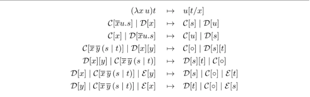
`The complete list of reduction rules of λ`is presented in Table 2 for the reader’s convenience. (λx u)t 7→ u[t/x] C[xu.s] | D[x] 7→ C[s] | D[u] C[x] | D[xu.s] 7→ C[u] | D[s] C[x y (s | t)] | D[x][y] 7→ C[◦] | D[s][t] D[x][y] | C[x y (s | t)] 7→ D[s][t] | C[◦] D[x] | C[x y (s | t)] | E[y] 7→ D[s] | C[◦] | E[t] D[y] | C[x y (s | t)] | E[x] 7→ D[t] | C[◦] | E[s]
Table 2: Reduction rules for NMLL terms.
As usual, for any context C[ ], we adopt the reduction scheme C[t] 7→ C[u] whenever t 7→ u. We denote by 7→∗ the reflexive and transitive closure of the one-step reduction 7→. As usual, we shall employ the λ-calculus concepts of normal form and strong normalization.
Definition 2.5 (Normal Forms and Strongly Normalizable Terms).
• A redex is a term u such that u 7→ v for some v and reduction in Table 2. A term t is called a normal form or, simply, normal, if there is no u such that t 7→ u.
• A finite or infinite sequence of terms u1, u2, . . . , un, . . . is said to be a
reduction of t, if t = u1, and for all i, ui 7→ ui+1. A term u of λ` is
normalizable if there is a finite reduction of u whose last term is normal and is strong normalizable if every reduction of u is finite.
3
Programming with λ
`In order to acquire familiarity with the main features of λ, we discuss now some programming examples. Namely, we shall see how to implement client-server communication, synchronization, cyclic communication patterns and channel sharing.
Example 3.1 (Client-Server: Request/Answer). In this example, we discuss how to represent in λ` a simple communication protocol, consisting in a re-quest/answer message exchange. A server hosts an online catalogue, mapping product names to prices. A client transmits a string prod : String to the server, representing a product name whose price the client wishes to know. The server answers the client request by sending back the price of the product prod, com-puted by the function cost : String ( N. A naive way to implement client and server would be CLIEN T z }| { xprod.y | SERV ER z }| { y(cost x).◦ Although, as expected
xprod.y | y(cost x).◦ 7→ y | y(cost prod).◦ 7→ y | y(price).◦ 7→ price | ◦ we observe that, this way, synchronization is implemented poorly. As we see below, the server may send to the client the message (cost x) before it receives any request whatsoever!
xprod.y | y(cost x).◦ 7→ xprod.cost x | ◦ = (λx cost x)prod | ◦ 7→∗price | ◦ What we expect, instead, is that only the request of the client can trigger com-putation and transmission of the answer by the server. In order to force that, the trick is to encapsulate the message prod into the λ-term λaλb a (b prod), whose task is to take as input a server channel a, a continuation b and apply the chan-nel a to b prod. We thus implement client and server as shown below on the left. Since the server output channel y. ◦ is not applied to any argument, the server has no choice but to wait for the client request, as shown below on the right.
CLIEN T z }| { x(λaλb a (b prod)).y | SERV ER z }| { x (y. ◦) cost
x(λaλb a (b prod)).y | x (y. ◦) cost 7→ y | (λaλb a (b prod)) (y. ◦) cost 7→∗y | (y(cost prod).◦
7→∗y | yprice.◦ 7→ price | ◦
By defining X := (N ( ⊥) ( (String ( N) ( ⊥, we can type the process above as follows:
x : X ⇒ x : X ⇒ y : N, y. ◦ : N ( ⊥
x : X ⇒ y : N, x (y. ◦) : (String ( N) ( ⊥ ⇒ cost : String ( N x : X ⇒ y : N, x (y. ◦) cost : ⊥
⇒ x. y : X ( N, x (y. ◦) cost : ⊥ ⇒ (λaλb a (b prod)) : X
⇒ x(λaλb a (b prod)).y : N, x (y. ◦) cost : ⊥ ⇒ x(λaλb a (b prod)).y | x (y. ◦) cost : N ` ⊥
Example 3.2 (Client-Server: Dialogue). We present now a continuation of the previous example which models a longer interaction. We want to represent the following transaction of an online sale. As before, a buyer transmits to a seller a product name prod : String, the seller computes by the function cost the monetary cost price : N of prod and communicates it to the buyer. Then the buyer applies a function pay : N → String to price, that will transmit to the server the credit card number card : String if the client wishes to buy the product, the empty string otherwise. By comparison with the previous example, we must add a new communication channel z for the third communication, because in λ` each communication requires a fresh channel. As before, in order to implement synchronization, messages M will be always transmitted as (λaλb a (b M )):
CLIEN T
z }| {
x(λaλb a (b prod)).y (z. ◦) pay |
SERV ER
z }| {
x (y. z) (λcλa0λb0a0(b0cost c)) We can observe the following interaction:
x(λaλb a (b prod)).y (z. ◦) pay | x (y. z) (λcλa0λb0a0(b0cost c)) 7→ y (z. ◦) pay | (λaλb a (b prod)) (y. z) (λcλa0λb0a0(b0cost c)) 7→∗y (z. ◦) pay | y((λcλa0λb0a0(b0cost c))prod).z
7→∗y (z. ◦) pay | y(λa0λb0a0(b0price)).z 7→ (λa0λb0a0(b0price)) (z. ◦) pay | z 7→∗z(pay price).◦ | z
7→ zcard.◦ | z 7→ ◦ | card
By defining X := (Y ( String) ( (String ( Y ) ( String, Y := (String ( ⊥) ( (N ( String) ( ⊥, we can type the process above as follows:
x : X ⇒ x : X
⇒ z : String, z. ◦ : String ( ⊥ y : Y ⇒ y : Y y : Y ⇒ y (z. ◦) : (N ( String) ( ⊥, z : String
⇒ y (z. ◦) : (N ( String) ( ⊥, y. z : Y ( String ⇒ pay : N ( String ⇒ y (z. ◦) pay : ⊥, y. z : Y ( String
x : X ⇒ y (z. ◦) pay : ⊥, x (y. z) : (String ( Y ) ( String ⇒ λcλa0λb0a0(b0
cost c) : String ( Y x : X ⇒ y (z. ◦) pay : ⊥, x (y. z)(λcλa0λb0a0(b0cost c)) : String
⇒ x. y (z. ◦) pay : X ( ⊥, x (y. z)(λcλa0λb0a0(b0cost c)) : String ⇒ λaλb a (b prod) : X
⇒ x(λaλb a (b prod)).y (z. ◦) pay : ⊥, x (y. z)(λcλa0λb0a0(b0cost c)) : String
⇒ x(λaλb a (b prod)).y (z. ◦) pay | x (y. z)(λcλa0λb0a0(b0cost c)) : ⊥` String
Example 3.3 (Cyclic Communication). Unlike in the session typed π-calculi of [10] and [37], in λ`one can type in a natural way cyclic communication patterns, as shown in the following example. A client has some secret information M : String, which it wishes to encrypt. For added security, the client desires two
encryptions of the message. A couple of servers, by joining forces, offer this kind of double-encryption service. Therefore, the client sends M to the first server, which encrypts M by applying the function enc1: String ( String and
then transmits the result to the second server, which in turn encrypts it by applying the function enc2: String ( String and finally transmits the result to
the client. The implementation is shown below on the left, and we observe the interaction shown below on the right.
CLIEN T z }| { xM.z | SERV ER 1 z }| { y(enc1x).◦ | SERV ER 2 z }| { z(enc2y).◦
xM.z | y(enc1x).◦ | z(enc2y).◦
7→ z | y(enc1M ).◦ | z(enc2y).◦
7→ z | yM0.◦ | z(enc2y).◦
7→ z | ◦ | z(enc2M0).◦
7→ z | ◦ | zM00.◦
7→ M00| ◦ | ◦ We can type the process above as follows:
⇒ z : String, z. ◦ : String ( ⊥ y : String ⇒ ◦ : ⊥, enc2y : String
y : String ⇒ z : String, ◦ : ⊥, z(enc2y).◦ : ⊥
⇒ z : String, y. ◦ : String ( ⊥, z(enc2y).◦ : ⊥ x : String ⇒ enc1x : String
x : String ⇒ z : String, y(enc1x).◦ : ⊥, z(enc2y).◦ : ⊥
⇒ x. z : String ( String, y(enc1x).◦ : ⊥, z(enc2y).◦ : ⊥ ⇒ M : String
⇒ xM.z : String, y(enc1x).◦ : ⊥, z(enc2y).◦ : ⊥
⇒ xM.z | y(enc1x).◦ : String` ⊥, z(enc2y).◦ : ⊥
⇒ xM.z | y(enc1x).◦ | z(enc2y).◦ : (String` ⊥) ` ⊥
Example 3.4 (Channel Transmission). Just like π-calculus, λ` supports com-munication of channel names and thus dynamic comcom-munication patterns, as we see in the following example. A server offers a printing service, which is hosted on another machine, connected to the server. In order to exploit the service an access code is required. A consumer, which wants to print the string M , sends its access code access : String to the server, which checks it by the function check. Upon success, the server transmits to the consumer the channel z along which the printer offers its services, so that finally the consumer can send M to the printer. We model printer, server and client as follows:
P RIN T ER z }| { z print | SERV ER z }| { (check x)(y. ◦)(z. ◦) | CON SU M ER z }| { xaccess.y (λa a M ) We observe the following interaction:
z print | (check x)(y. ◦)(z. ◦) | xaccess.y (λa a M ) 7→ z print | (check access)(y. ◦)(z. ◦) | y (λa a M ) 7→ z print | y(z. ◦).◦ | y (λa a M )
7→ z print | ◦ | z(λa a M ).◦ 7→ (λa a M ) print | ◦ | ◦ 7→ print M | ◦ | ◦
By defining C := ((String ( ⊥) ( ⊥) ( ⊥, we can type the above process as follows:
x : String ⇒ check x : C ( C ( ⊥
y : C ⇒ ◦ : ⊥, y (λa a M ) : ⊥ ⇒ y. ◦ : C, y (λa a M ) : ⊥ x : String ⇒ (check x)(y. ◦) : C ( ⊥, y (λa a M ) : ⊥
⇒ (check x)(y. ◦) : C ( ⊥, x. y (λa a M) : String ( ⊥ ⇒ access : String ⇒ (check x)(y. ◦) : C ( ⊥, xaccess.y (λa a M) : ⊥ ⇒ z print : ⊥, z. ◦ : C
⇒ z print : ⊥, (check x)(y. ◦)(z. ◦) : ⊥, xaccess.y (λa a M ) : ⊥ ⇒ z print | (check x)(y. ◦)(z. ◦) : ⊥` ⊥, xaccess.y (λa a M) : ⊥ ⇒ z print | (check x)(y. ◦)(z. ◦) | xaccess.y (λa a M ) : (⊥` ⊥) ` ⊥
4
Intermezzo: Synchronous Communication in
λ
`In π-calculus the actions of both sending and receiving messages are synchronous and blocking. They are synchronous, because they require that the sender and the receiver synchronize; they are blocking, because the execution of both the sender and the receiver is blocked until the message is actually transmitted. Therefore, on one hand, if there is no receiver listening to the channel, a pro-cess can neither transmit its message along the channel nor proceed with its execution. On the other hand, a process which does listen cannot proceed with its execution until it receives the message it is waiting for. In π-calculus, syn-chronicity is implemented by a construct for sending xm. and a construct for receiving x(y). which need to be outermost in the connected processes in order to activate the reduction: xm.P | x(y).Q 7→ P | Q[m/y]. The blocking nature of the actions is implemented by forbidding reductions inside P and Q before the actions are executed, that is, by forcing a reduction strategy.
Non-blocking actions have been advocated by various authors (e.g. [25], [21]) and are necessary for a full correspondence between cut-elimination and process execution. In λ`, the fact that sending and receiving are non-blocking is implemented by just removing the input construct x(y). Hence, provided that x occurs in Q, in λ` we have:
xm.P | Q 7→ P | Q[m/x]
4.1
The Call-by-Value λ
`Although λ`is naturally asynchronous, we can model synchronous and blocking actions also in λ`, by defining reduction to automatically follow a call-by-value discipline.
Definition 4.1 (Value). A value is any term of one of the following forms: x. t s | t
Definition 4.2 (Call-by-value Contexts). We define a call-by-value evalua-tion context by the following grammar:
E := [ ] | E u | V E | x y E | close(E) where V is any value.
To obtain a call-by-value version of λ`, we rewrite the main reduction rules of λ` as follows:
. . . | E[(λx u)V ] | . . . 7→cbv. . . | E[u[V /x]] | . . .
. . . | E[xV.s] | . . . | E0[x] | . . . 7→cbv . . . | E[s] | . . . | E0[V ] | . . .
. . . | E0[x] | . . . | E[xV.s] | . . . 7→cbv. . . | E0[V ] | . . . | E[s] | . . .
where V is a value and E, E0call-by-value evaluation contexts. The reduction for x y V are analogous. The idea is that call-by-value contexts bring back a notion of order among operations, which can be used to represent the sequential facet of computation. Thus a term E0[x] represents a process whose next operation
is a read operation on the channel x, followed by the operations contained in E0[ ]. Similarly to Wadler’s principal-cut-elimination strategy for CP, 7→cbvonly
allows communication on the top level parallel operators.
We can now define in λ` the synchronous input-construct as follows: x(y).u := (λy u) x
Indeed, the term x(y).u is always stuck: since u is located under a λ, no reduc-tion can be performed inside u; since x is not a value, the redex (λy u) x cannot be contracted either. For similar reasons, the term xV.u = (x. u)V is stuck as well: since V is a value, no reduction can be performed inside V ; since u is lo-cated under an output operator, no reduction can be performed inside u either. Thus, the only reduction that could be fired is the transmission of V along the channel x, which however requires a suitable receiver, namely a process whose call-by-value evaluation cannot further proceed: the process requires an input value and waits for it. Indeed, in the following configuration, we can reduce
xV.u | x(y).w = xV.u | (λy w)x 7→cbvu | (λy w)V 7→cbv u | w[V /y] In the configuration
xV.u | (λz z x(y).w)(λk k)
however, the process xV.u cannot transmit its message V until (λz z x(y).w)(λk k) is ready to receive, which will happen as soon as its head redex will be contracted and the value of x(y).w will be really needed. Thus, after one reduction step, we have
5
Soundness and Completeness
We show now that the typing system NMLL of λ` captures exactly classical multiplicative linear logic. Namely, we show that NMLL is equivalent to the sequent calculus MLL for classical multiplicative linear logic. The cut rule and the logical rules of MLL – namely, the rules introducing the logical connectives of linear logic on the left or on the right – are the standard double-sided sequent rules for classical linear logic. The initial sequent ⊥ ⇒ corresponds to the initial sequent ⇒ 1. We use the former since we do not use an explicit duality operator. The only non-standard rule of NMLL is ⊥E. It is clearly sound since it captures the neutrality of ⊥ with respect to`, and hence to the comma on the right-hand side of sequents. Γ ⇒ ∆ Γ ⇒ ∆, ⊥ ⊥ ⊥ ⇒ Γ ⇒ A, ∆ Σ, B ⇒ Θ Γ, Σ, A ( B ⇒ ∆, Θ ( l Γ, A ⇒ B, ∆ Γ ⇒ A ( B, ∆ ( r Γ, A ⇒ ∆ Σ, B ⇒ Θ Γ, Σ, A` B ⇒ ∆, Θ `l Γ ⇒ A, B, ∆ Γ ⇒ A` B, ∆ `r Γ ⇒ A, ∆ Σ, A ⇒ Θ Γ, Σ ⇒ ∆, Θ cut
Table 3: The sequent calculus MLL.
Proposition 5.1 (Soundness). If Γ ⇒ ∆ is derivable in NMLL, then Γ ⇒ ∆ is derivable in MLL.
Proof. By induction on the number of rule applications in the NMLL derivation of S = Γ ⇒ ∆.
The natural deduction calculus NMLL corresponds very neatly to the se-quent calculus MLL. Hence, a completeness proof of NMLL with respect to MLL is quite straightforward. The proof deviates from standard reasoning only insofar as we need to handle the occurrences of ⊥ introduced by`E. Indeed, whenever we apply`E, we introduce an occurrence of ⊥ to type a term of the form x y m containing output channels x and y and a message m. But, in order to obtain a derivation of a specific target sequent Γ ⇒ ∆, we might need to remove those extra occurrences of ⊥. To do so, we use the ⊥E rule.
Proposition 5.2 (Completeness). If Γ ⇒ ∆ is derivable in MLL, then Γ ⇒ ∆ is derivable in NMLL.
Proof. By induction on the number of rule applications in the MLL derivation of S = Γ ⇒ ∆.
6
Subject Reduction
We are now going to prove that the reductions of λ` preserve the typing of terms, a property well-known under the name of Subject Reduction. We first need the concept of substitution, which in λ` is just a replacement of some variables, with no renaming involved.
Definition 6.1 (Substitution). For any multiset of typed terms ∆ and terms v1, . . . , vn, we denote by ∆[v1/x1 . . . vn/xn] the simultaneous replacement,
for any i ∈ {1, . . . , n}, of all occurrences of xi in all terms of ∆ by vi. Given a
substitution [t/x], we refer to t as the substituting term and to x as the substituted variable.
In order to prove Subject Reduction, we first prove that if we have a variable x : A in the context of a derivable sequent Γ, x : A ⇒ ∆ and we can type a term t : A by deriving a sequent Σ ⇒ t : A, Θ, then we can derive the sequent Γ, Σ ⇒ ∆[t/x], Θ effectively replacing the variable x : A with the term t : A. The proof-theoretical intuition is the following: if A is among the assumptions of a proof, and we have a derivation t of A, then we can use t to derive A directly inside the proof.
Lemma 6.1 (Substitution). If Σ ⇒ t : A, Θ and Γ, x : A ⇒ ∆ are derivable in NMLL and share no variable, then Γ, Σ ⇒ ∆[t/x], Θ is derivable in NMLL as well.
Proof. We proceed by induction on the number of rule applications in the deriva-tion of Γ, x : A ⇒ ∆.
If no rule is applied in the derivation, then Γ, x : A ⇒ ∆ is of the form x : A ⇒ x : A. Therefore, Γ, Σ ⇒ ∆[t/x], Θ is just Σ ⇒ t : A, Θ and the claim trivially holds.
Suppose now that the statement holds for any sequent which is derivable with n or less rule applications, we show the result for any sequent Γ, x : A ⇒ ∆ which is derivable using n + 1 rule applications. We reason by cases on the last rule applied in this derivation of Γ, x : A ⇒ ∆.
• Γ, x : A ⇒ ∆ 0 Γ, x : A ⇒ ∆0, ◦ : ⊥ ⊥I where ∆ = ∆ 0, ◦ : ⊥. By inductive hypothesis Γ, Σ ⇒ ∆0[t/x], Θ is derivable. By applying Γ, Σ ⇒ ∆0[t/x], Θ Γ, Σ ⇒ ∆0[t/x], Θ, ◦ : ⊥ ⊥I
we obtain a derivation of Γ, Σ ⇒ ∆[t/x], Θ, which verifies the claim. The rule ⊥E is similar.
• Γ1⇒ v : B ( C, ∆1 Γ2⇒ w : B, ∆2
Γ1, Γ2⇒ vw : C, ∆1, ∆2 ( E where ∆ = vw : C, ∆ 1, ∆2.
Suppose that x : A is contained in Γ1 and hence that Γ1 = Γ01, x : A
analogous. By inductive hypothesis Γ01, Σ ⇒ v[t/x] : B ( C, ∆1[t/x], Θ
is derivable. Now, due to the type assignment rules of NMLL and since x : A is contained in Γ1, we have that x cannot occur in w. By hypothesis,
t and Θ share no variable with Γ2, w, ∆2. Hence, by applying
Γ1, Σ ⇒ v[t/x] : B ( C, ∆1[t/x], Θ Γ2⇒ w : B, ∆2
Γ1, Σ, Γ2⇒ (v[t/x])w : C, ∆1[t/x], Θ, ∆2 ( E
we obtain a derivation of Γ, Σ ⇒ (vw)[t/x] : C, ∆[t/x], Θ, which verifies the claim.
• Γ, y : B ⇒ s : C, ∆
0
Γ ⇒ y. s : B ( C, ∆0 ( I where ∆ = y. s : B ( C, ∆
0. Since x : A must
occur in Γ in the conclusion of the rule application, we know that x 6= y. By inductive hypothesis, Γ, y : B, Σ ⇒ s[t/x] : C, ∆0[t/x], Θ is derivable. Hence, since by hypothesis y does not occur in t, by applying
Γ, y : B, Σ ⇒ s[t/x] : C, ∆0[t/x], Θ Γ, Σ ⇒ y. (s[t/x]) : B ( C, ∆0[t/x], Θ ( I
we obtain a derivation of Γ, Σ ⇒ (y. s)[t/x] : B ( C, ∆0[t/x], Θ, which verifies the claim.
• The cases`E and `I are similar.
The proof of the Subject Reduction is now quite standard.
Theorem 6.2 (Subject Reduction). Assume there is a NMLL derivation of Π ⇒ t1: F1, . . . , tn: Fn, tn+1, . . . , tm. If t1| . . . | tm 7→ t01| . . . | t0m, then there
is a derivation of Π ⇒ t01: F1, . . . , t0n: Fn, t0n+1, . . . , t0m.
Proof. We prove the statement by induction on the number of rule applications in the derivation of Π ⇒ t1: F1, . . . , tn: Fn, tn+1, . . . , tm.
If no rule is applied in the derivation, then Π ⇒ t1: F1, . . . , tn: Fn, tn+1, . . . , tm
is of the form x : A ⇒ x : A. Since no reduction applies to any term in the right-hand side of the sequents, the claim trivially holds.
Suppose now that the statement holds for any NMLL derivation containing m or less rule applications, we show the result for a generic NMLL derivation of Π ⇒ t1: F1, . . . , tn: Fn, tn+1, . . . , tmcontaining m + 1 rule applications. We
reason by cases on the last rule applied in this NMLL derivation. • Γ ⇒ x. v : A ( B, ∆ Σ ⇒ w : A, Θ
Γ, Σ ⇒ xw.v : B, ∆, Θ ( E where t1| . . . | tm = t1| . . . | xw.v | . . . | tm
and
t01| . . . | t0m = (t1| . . . | v | . . . | tm)[w/x]
– If the last rule applied above Γ ⇒ x. v : A ( B, ∆ is Γ, x : A ⇒ v : B, ∆
Γ ⇒ x. v : A ( B, ∆ ( I
then, by the restriction on NMLL rule applications, x occurs either in v or in ∆, and by Lemma 6.1 applied to the sequents Σ ⇒ w : A, Θ and Γ, x : A ⇒ v : B, ∆ we obtain that Γ, Σ ⇒ v[w/x] : B, ∆[w/x], Θ is derivable and hence that we have a derivation of Π ⇒ t01: F1, . . . , t0n: Fn, t0n+1, . . . , t0m.
– Otherwise, we have
Φ1⇒ x. v : A ( B, Ψ1 . . . Φp⇒ Ψp
Γ ⇒ x. v : A ( B, ∆ ρ Σ ⇒ w : A, Θ Γ, Σ ⇒ xw.v : B, ∆, Θ ( E
where x. v : A ( B only occurs in one of the premises of ρ – we display it in the first premise without loss of generality.
If we construct the following derivation
Φ1⇒ x. v : A ( B, Ψ1 Σ ⇒ w : A, Θ
Φ1, Σ ⇒ xw.v : B, Ψ1, Θ ( E . . . Φp⇒ Ψp Γ, Σ ⇒ xw.v : B, ∆, Θ ρ
we know without loss of generality that
xw.v : B, Ψ1, Θ = t1: F1, . . . , tj : Fj, tn+1, . . . , ti and that t1| . . . | tj | tn+1| . . . | tl 7→ t01| . . . | t 0 j| t 0 n+1| . . . | t 0 i
because by Proposition 7.1, x occurs either in v or in Ψ1. By inductive
hypothesis, there is a derivation of
Φ1, Σ ⇒ t01: F1, . . . , t0j : Fj, t0n+1, . . . , t 0 i = Φ1, Σ ⇒ v[w/x] : B, Ψ1[w/x], Θ By assumption we have Γ, Σ ⇒ xw.v : B, ∆, Θ = Π ⇒ t1: F1, . . . , tn : Fn, tn+1, . . . , tm
Therefore, by inspection of the rules of NMLL, it is easy to see that by the rule application
Φ1, Σ ⇒ v[w/x] : B, Ψ1[w/x], Θ . . . Φp⇒ Ψp
Γ, Σ ⇒ v[w/x] : B, ∆[w/x], Θ ρ we obtain a derivation of the sequent
Γ, Σ ⇒ v[w/x] : B, ∆[w/x], Θ = Γ, Σ ⇒ t01: F1, . . . , t0n: Fn, t0n+1, . . . , t 0 m
• Γ ⇒ v | w : A` B, ∆ Σ1, x : A ⇒ Θ1 Σ2, y : B ⇒ Θ2
Γ, Σ1, Σ2⇒ x y (v | w) : ⊥, ∆, Θ1, Θ2 `E where
t1| . . . | tm = t1| . . . | x y (v | w) | . . . | tm
and
t01| . . . | t0m = (t1| . . . | ◦ | . . . | tm)[v/x w/y]
– If the last rule applied above Γ ⇒ v | w : A` B, ∆ is Γ ⇒ v : A, w : B, ∆
Γ ⇒ v | w : A` B, ∆ `I
By the application of Lemma 6.1 to the sequents Γ ⇒ v : A, w : B, ∆ and Σ1, x : A ⇒ Θ1 we obtain that Γ, Σ1 ⇒ w : B, ∆, Θ1[v/x]
is derivable. Furthermore, by applying Lemma 6.1 to the sequents Γ, Σ1 ⇒ w : B, ∆, Θ1[v/x] and Σ2, y : B ⇒ Θ2 we obtain that
Γ, Σ1, Σ2 ⇒ ∆, Θ1[v/x], Θ2[w/y]. Since x occurs in Θ1 and y
oc-curs in Θ2, we can construct a derivation of Π ⇒ t01 : F1, . . . , t0n :
Fn, t0n+1, . . . , t0mby applying ⊥I. – Otherwise, we have Φ1⇒ v | w : A` B, Ψ1 . . . Φp⇒ Ψp Γ ⇒ v | w : A` B, ∆ ρ Σ1, x : A ⇒ Θ1 Σ2, y : B ⇒ Θ2 Γ, Σ ⇒ x y (v | w) : ⊥, ∆, Θ1, Θ2 `E
where v | w : A` B only occurs in one of the premises of ρ – we display it in the first premise without loss of generality.
If we construct the following derivation
Φ1⇒ v | w : A` B, Ψ1 Σ1, x : A ⇒ Θ1 Σ2, y : B ⇒ Θ2
Φ1, Σ ⇒ x y (v | w) : ⊥, Ψ1, Θ1, Θ2 `E . . . Φp⇒ Ψp
Γ, Σ ⇒ x y (v | w) : ⊥, ∆, Θ1, Θ2
ρ
we know without loss of generality that
x y (v | w) : ⊥, Ψ1, Θ1, Θ2 = t1: F1, . . . , tj : Fj, tn+1, . . . , ti
and that
t1| . . . | tj| tn+1| . . . | ti 7→ t01| . . . | t0j| t0n+1| . . . | t0i
because x and y occur in Θ1 and Θ2 respectively. By inductive
hypothesis, there is a derivation of Φ1, Σ ⇒ t01: F1, . . . , t0j: Fj, t0n+1, . . . , t
0
i = Φ1, Σ ⇒ ◦ : ⊥, Ψ1, Θ1[v/x], Θ2[w/y]
By assumption
Therefore, by the rule application
Φ1, Σ ⇒ ◦ : ⊥, Ψ1, Θ1[v/x], Θ2[w/y] . . . Φp⇒ Ψp Γ, Σ ⇒ ◦ : ⊥, ∆, Θ1[v/x], Θ2[w/y] ρ
we have a derivation of the sequent
Γ, Σ ⇒ ◦ : ⊥, ∆, Θ1[v/x], Θ2[w/y] = Γ, Σ ⇒ t01: F1, . . . , t0n: Fn, t0n+1, . . . , t 0 m
• In all other cases, the term xw.v (or x y v) that triggered the reduction t1| . . . | tm7→ t01| . . . | t0malready occurs in the premises of the last rule ρ
applied in the NMLL derivation of Π ⇒ t1: F1, . . . , tn: Fn, tn+1, . . . , tm.
According to the typing rules, no variable can occur in different premises of the same rule application. Therefore, both the term xw.v (respectively y z v) and the variable x (respectively y and z) occur inside the same premise of the last rule application
Γ ⇒ u1: G1, . . . , up: Gp . . . Φ ⇒ Ψ
Σ ⇒ ∆, C1[u1] : Fj, . . . , Cp[up] : Fn
ρ
in the derivation of
Σ ⇒ ∆, C1[u1] : Fj, . . . , Cp[up] : Fn = Π ⇒ t1: F1, . . . , tn: Fn, tn+1, . . . , tm
Without loss of generality, we assume that x (or y and z) occurs in the premise
Γ ⇒ u1: G1, . . . , up: Gp
By reducing the redex triggered by xw.v or x y v in the term u1| . . . | up
we have u1 | . . . | up 7→ u01 | . . . | u0p. By inductive hypothesis, there is
a derivation of Γ ⇒ u01 : G1, . . . , u0p : Gp. Now, by inspection of NMLL
typing rules, we can easily see that t1| . . . | tm is of the form D[ C1[u1] |
. . . | Cp[up] ] and by assumption
t01| . . . | t0m= D[ C1[u01] | . . . | Cp[u0p] ]
Therefore, by inspection of the rules of NMLL, it is easy to see that by the application of ρ
Γ ⇒ u01: G1, . . . , u0p: Gp . . . Φ ⇒ Ψ
Σ ⇒ ∆, C1[u01] : Fj, . . . , Cp[u0p] : Fn
ρ
to the root of the derivation of Γ ⇒ u01 : G1, . . . , u0p : Gp, we obtain a
derivation of
Σ ⇒ ∆, C1[u01] : Fj, . . . , Cp[u0p] : Fn = Π ⇒ t01: F1, . . . , t0n: Fn, t0n+1, . . . , t 0 m
7
Progress
We show now that λ` is deadlock-free: if a process contains a potential com-munication, then the term is not normal and the communication will be carried out. In λ`, potential communications are represented by subterms of the form xv.w or x y v. Indeed, the presence of those subterms in a process means that the process can use a communication channel x – or a pair of channels x and y – to transmit a message v. Thus we need to show that if such a subterm occurs in a term, there is also a receiver and the term is not normal. We start by show-ing some properties of the distribution of variables inside NMLL sequents and inside typed λ`-terms. The crucial property is that an output communication channel x can only occur if there is a corresponding input channel x.
Proposition 7.1 (Linearity of Channels). Assume Γ ⇒ ∆ is derivable in NMLL and let x be any variable. Then:
• if x occurs in Γ, x occurs exactly once in ∆ and x does not occur in ∆; • if x does not occur in Γ but occurs in ∆, x occurs exactly once as x and
exactly once as x in ∆.
Proof. By straightforward induction on the length of the derivation of Γ ⇒ ∆.
We recall that by Definition 2.4 a simple context C[ ] is a process which is not a direct parallel composition of simpler processes. A crucial property of simple contexts that we are going to obtain now is the following: if C[zu.v] is typable and C[ ] is simple, then the variable z cannot occur in C[ ]. If such a configuration were possible, we might type λ`-terms like z(zu.v) and we would have to choose between allowing components of the same process reduction to communicate z(zu.v) 7→ uv or tolerating a deadlock. Fortunately, the next proposition rules out this scenery.
Proposition 7.2. Suppose Φ ⇒ C[u] : F, Π or Φ ⇒ C[u], Π is derivable in NMLL. Then, if C[ ] is simple and the variable z occurs in u, then z does not occur in C[ ].
Proof. We prove the statement by induction on the number of rule applications in the derivation of Φ ⇒ C[u] : F, Π or Φ ⇒ C[u], Π.
If C[ ] is empty, we are done.
If no rule is applied in the derivation, then Φ ⇒ C[u] : F, Π or Φ ⇒ C[u], Π is of the form x : A ⇒ x : A, thus u = x and C[ ] is empty, therefore the claim trivially holds.
Suppose now that the statement holds for any NMLL derivation containing m or less rule applications, we show the result for a generic NMLL derivation containing m + 1 rule applications. We reason by cases on the last rule applied in this NMLL derivation. We may assume that the term C[u] does not occur in any premise of this last rule, otherwise we just apply the inductive hypothesis to any premise containing C[u] and obtain the thesis.
• Γ ⇒ ∆
Γ ⇒ ∆, ◦ : ⊥ ⊥I. Since C[u] occurs in ∆, this case is ruled out by our assumption that C[u] does not occur in Γ ⇒ ∆.
• Γ ⇒ ∆, t : ⊥
Γ ⇒ ∆, close(t) ⊥E. By our assumption, it must be the case that C[u] = close(t). If C[ ] = close([ ]), surely z does not occur in C[ ]. If C[ ] = close(D[ ]), with t = D[u], then by inductive hypothesis, z does not occur in D[ ], thus it does not occur in C[ ] = close(D[ ]) either.
• Γ ⇒ t : A ( B, ∆ Σ ⇒ s : A, Θ
Γ, Σ ⇒ ts : B, ∆, Θ ( E. By our assumption, it must be the case that C[u] = ts. Therefore, t = D[u] or s = D[u], with respectively C[ ] = D[ ] s and C[ ] = t D[ ]. By inductive hypothesis, z does not occur in D[ ]. Moreover, since the premises of the typing rule share no variable, z cannot occur respectively in s and t. Therefore, z does not occur in C[ ]. • Γ, x : A ⇒ t : B, ∆
Γ ⇒ x. t : A ( B, ∆ ( I. By our assumption, it must be the case that C[u] = x. t. Therefore, t = D[u] and C[ ] = x. D[ ]. By inductive hypoth-esis, z does not occur in D[ ]. Moreover, z 6= x, otherwise z would occur twice in x. t, contradicting Proposition 7.1. Therefore, z does not occur in C[ ] = x. D[ ].
• Γ ⇒ t : A` B, ∆ Σ1, x : A ⇒ Θ1 Σ2, y : B ⇒ Θ2
Γ, Σ1, Σ2⇒ x y t : ⊥, ∆, Θ1, Θ2 `E. By our
as-sumption, it must be the case that C[u] = x y t. Therefore, t = D[u] and C[ ] = x y D[ ]. By inductive hypothesis, z does not occur in D[ ]. Moreover, z 6= x, y, otherwise z would occur twice in x y t, contradicting Proposition 7.1. Therefore z does not occur in C[ ] = x y D[ ].
• Γ ⇒ t : A, s : B, ∆
Γ ⇒ t | s : A` B, ∆ `I. We claim that this case is not possible. Indeed, if it were, by our assumption we would have C[u] = t | s. Therefore t = D[u] or s = D[u], with respectively C[ ] = D[ ] | s and C[ ] = t | D[ ]. Since by Definition 2.4 the context C[ ] would not be simple, we would have a contradiction.
It is now easy to show that if a communication is possible, it will be carried out: if a typable λ`-term contains output channels ready to transmit messages, then it can always perform the communication, because there is always a suitable receiver.
Theorem 7.3 (Progress).
1. Suppose Γ ⇒ C[xv.u] : F, t1: F1, . . . , tn : Fn, tn+1, . . . , tm is derivable
2. Suppose Γ ⇒ C[x y u] : F, t1: F1, . . . , tn : Fn, tn+1, . . . , tm is derivable
in NMLL. Then the term C[x y u] | t1| . . . | tm is not normal.
Proof. 1. By Proposition 7.1, x and x must occur exactly once in the term C[xv.u] | t1| . . . | tm. If x occurs in some ti, then a reduction is possible and we
are done. We assume therefore that x occurs in C[xv.u]. We also assume C[ ] is empty, otherwise x occurs in u, hence xv.u = (λx u)v, which is not normal and we are done.
We claim now that C[xv.u] has a subterm of the form E [xv.u] | D[x] or D[x] | E[xv.u], which implies a communication reduction is possible, allowing us to conclude the proof. We prove our claim by induction on C[xv.u].
If C[xv.u] = z. C0[xv.u] or C[xv.u] = y z C0[xv.u] or C[xv.u] = close(C0[xv.u]), then we apply the induction hypothesis on C0[xv.u], and we are done.
If C[xv.u] = w C0[xv.u] or C[xv.u] = C0[xv.u] w, then by Proposition 7.2, x must occur in C0[xv.u], hence we apply the induction hypothesis on C0[xv.u], and we are done.
If C[xv.u] = C0[xv.u] | w or C[xv.u] = w | C0[xv.u], then if x occurs in w, we are done. Otherwise, we apply the induction hypothesis on C0[xv.u], and concluding the proof of the claim.
2. By Proposition 7.1, x and x must occur both exactly once in the term C[x y u] | t1| . . . | tm and so do y and y. By inspection of the inference rules of
NMLL it is easy to see that x, y cannot occur in u, therefore they occur in some ti. Thus, a reduction is possible.
8
The Subformula Property
We show in this section that each normal λ`-term corresponds to an analytic derivation: the type of each subterm of any normal λ`-term t is either a sub-formula of the type of t or a subsub-formula of the types of the variables of t. This property guarantees that, proof-theoretically, the reduction rules of λ` give rise to a complete detour removal procedure, hence we can conclude they are also satisfactory from a logical point of view. Indeed, without this property it is not possible to relate normalization and cut-elimination, as a normal proof without the subformula property cannot be translated in to a cut-free proof. NMLL can then be considered as a well-behaved alternative to sequent calculus and proof-nets for multiplicative linear logic.
We start by defining what it means for a derivation to be in normal form. Definition 8.1 (Normal form). An NMLL derivation of a sequent Γ ⇒ t1 :
T1, . . . , tn : Tn, tn+1, . . . , tm is in normal form if the term t1 | . . . | tm is in
normal form.
We then recall the notion of stack [22]. A stack represents, from a logical perspective, a series of elimination rules, from a computational perspective, a series of tasks to be carried out.
Definition 8.2 (Stack). A stack is a possibly empty sequence σ = ξ1ξ2. . . ξn
such that for every 1 ≤ i ≤ n, ξi= t, with t term of NMLL. If t is a proof term,
t σ denotes as usual the term (((t ξ1) ξ2) . . . ξn).
Before proving the Subformula Property, we need to establish two auxiliary results concerning the shape of terms. The first of these two results guarantees that the expected connection between the shape of a term with its type holds. Proposition 8.1 (Type coherence). If Γ ⇒ t : F, ∆ is derivable in NMLL and t is a value, then either t = x. t and F = A ( B or t = s | t and F = A ` B, for some types A and B.
Proof. By induction on the number of rule applications in the derivation of Γ ⇒ t : F, ∆.
The second auxiliary result establishes that any normal λ`-term – the type of which is not ⊥ – is either a value or a sequence of operations that cannot be carried out.
Lemma 8.2 (The shape of normal terms). If there is a derivation in NMLL of Γ ⇒ u : F, Π, where u is in normal form, is not a value and F 6= ⊥, then u = yσ.
Proof. By induction on the number of rule applications in the derivation of Γ ⇒ u : F, Π.
We can now show that normal λ`-terms satisfy the Subformula Property. The proof is by induction on the size of the NMLL derivation and, as usual, the difficult case is the one involving implication elimination. Even though we handle this case by a standard argument on the type of sequences of eliminations, represented here by stacks, the multiple-conclusion setting forces us to integrate this argument in the main induction. We do so by using a stronger inductive statement that carries along the induction the required statement about the type of stacks.
Theorem 8.3 (Subformula Property). Consider any normal NMLL derivation P of the sequent x1 : X1, . . . , xm : Xm⇒ t1 : T1, . . . , tn : Tn, Π, where Π does
not contain any type. Then every type S occurring in P is a subformula of some type T1, . . . , Tn or X1, . . . , Xmor ⊥.
Proof. We prove a stronger statement:
Consider any normal NMLL derivation P of the sequent x1: X1, . . . , xm:
Xm ⇒ t1 : T1, . . . , tn : Tn, Π, where Π does not contain any type.
Then every type S occurring in P is a subformula of some type T1, . . . , Tn or X1, . . . , Xm or ⊥. Moreover, if a term ti with i ∈
{1, . . . , n} is of the form yσ where σ is a stack, then Ti is a
subfor-mula of some type T1, . . . , Ti−1, Ti+1, . . . , Tn or X1, . . . , Xm or ⊥.
9
Strong Normalization
It is quite immediate to see that all terms of the calculus strongly normalize. Indeed, each reduction step strictly decreases the size of the term. This is due to the linear nature of terms (Proposition 7.1): each communication or λ-reduction moves one or two terms from one location to another. Therefore, no duplication is involved in the reductions. Since, moreover, each reduction removes one binder from the term, we have that the size of the term strictly decreases. We formally show this in the following theorem.
Definition 9.1 (Communication-size of a term). For any term t, its communi-cation size cs(t) is the number of occurrences of x. and x y in t.
Theorem 9.1 (Strong normalization). For any term t such that Γ ⇒ t : F is derivable in NMLL, all sequences of terms t1, t2. . . such that t1 = t and
ti7→ ti+1 are finite and contain exactly cs(t) terms.
Proof. The proof is by induction on the communication-size cs(t) of t.
10
Confluence
We show now that each λ`-term has a unique normal form. Since all λ`-terms have a normal form, this implies that the calculus λ`is confluent: for any term t, if t 7→ t0 and t 7→ t00, then there is a term t? such that both t0 7→ t? and
t007→ t?.
In order to simplify the proof of confluence, we define the concept of acti-vator. Intuitively, the activator of a reduction is the term which is responsible for the reduction. For instance, to trigger a communication we only need a subterm which is ready to send a message, such as xw.v. If we do trigger this communication of w through x, the term xw.v is going to be its activator. Definition 10.1 (Activator). Given any reduction s 7→ t, we say that the activator of s 7→ t is the subterm of s of the form (λx v)w, xw.v, y z v, which is displayed in the corresponding reduction.
Theorem 10.1 (Uniqueness of the normal form). For any term t such that the sequent Γ ⇒ t : F is derivable in NMLL, t has only one normal form.
Proof. The proof is by induction on the length of the normalization of t. If cs(t) = 0, the claim trivially holds. We show the claim for a generic term t such that cs(t) = m + 1, under the assumption that the claim holds for all terms with communication-size m or less.
Suppose that the term t reduces to two different terms t0 and t00if we reduce two different redexes in t. We show that both t0 and t00can reduce to the same term t?. Since, by inductive hypothesis, t0has a unique normal form and t00 has a unique normal form as well, this is enough to show that t has a unique normal form. Since the argument for the`-reductions is everywhere close to identical
to the argument for (-reductions, we only present the latter. Let us denote then the reduction t 7→ t0 as
u1| . . . | C[xw.v] | . . . | un 7→ ( u1| . . . | C[v] | . . . | un)[w/x]
There are two main cases.
1. If one of the activators of t 7→ t0 and t 7→ t00 is a subterm of the other, we consider the outermost activator. Without loss of generality, we assume that the outermost is the activator of t 7→ t0. Now, the activator yr.s of t 7→ t00 is
either a subterm of v or of w.
• The activator of t 7→ t00 is a subterm of v. The reduction t 7→ t00is then of
the form
u1| . . . | C[xw.v] | . . . | un 7→ (u1| . . . | C[xw.v0] | . . . | un)[r/y]
where v0 is obtained from v by replacing yr.s with s. Since, by Proposi-tion 7.2, y does not occur in w, we have t007→ t?, with
t?:= ((u1| . . . | C[v0] | . . . | un)[r/y])[w/x]
We just need to show that t0 7→ t?, that is
( u1| . . . | C[v] | . . . | un)[w/x] 7→ ((u1| . . . | C[v0] | . . . | un)[r/y])[w/x]
By Proposition 7.1 we have that y 6= x. Now, if r contains x,
(u1| . . . | C[v] | . . . | un)[w/x] = (u1| . . . | C[v[w/x]] | . . . | un) 7→ ( u1| . . . | C[v0] | . . . | un)[r[w/x]/y] = t?
If r does not contain x and since y does not occur in w, we have
(u1| . . . | C[v] | . . . | un)[w/x] 7→ ( u1| . . . | C[v0] | . . . | un)[w/x][r/y] = t?
• The activator of t 7→ t00 is a subterm of w. The reduction t 7→ t00 is then
of the form
u1| . . . | C[xw.v] | . . . | un 7→ (u1| . . . | C[(xw0.v] | . . . | un)[r/y]
where w0 is obtained from w by replacing yr.s with s. We have t007→ t?,
with
t?:= ((u1| . . . | C[v] | . . . | un)[r/y])[w0[r/y]/x]
We just need to show that t0 7→ t?, that is
( u1 | . . . | C[v] | . . . | un)[w/x] 7→ ((u1| . . . | C[v] | . . . | un)[r/y])[w0[r/y]/x]
We have the following reduction:
(u1| . . . | C[v] | . . . | un)[w/x] 7→ (( u1| . . . | C[v] | . . . | un)[w0/x])[r/y]
Now, r does not contain x, by Proposition 7.2 and because the activator of t 7→ t00 occurs in w. Since, moreover, y 6= x, we also have
(( u1| . . . | C[v] | . . . | un)[w0/x])[r/y] = (( u1| . . . | C[v] | . . . | un)[r/y])[w0[r/y]/x]
2. If neither of the activators of t 7→ t0 and t 7→ t00 is a subterm of the other, the reduction t 7→ t00 is of the form
u1| . . . | C[xw.v] | . . . | un 7→ (u01| . . . | C 0
[xw.v] | . . . | u0n)[r/y]
where u0i and C0[ ] are either equal to, respectively, ui and C[ ] or obtained from
ui and C[ ], respectively, by replacing the activator yr.s of t 7→ t00 with s. We
have t007→ t?, with
t?:= ((u01| . . . | C0[v] | . . . | u0n)[r/y])[w[r/y]/x] We just need to show that t07→ t?, that is
( u1| . . . | C[v] | . . . | un)[w/x] 7→ ((u01| . . . | C 0
[v] | . . . | u0n)[r/y])[w[r/y]/x]
Now, if s is the activator of a reduction, also s[w/x] has the suitable shape to be one; and the relative reductions substitute the same variable. By Definition 2.3, moreover, y 6= x and hence y occurs in the term ( u1| . . . | C[v] | . . . | un)[w/x],
and we can reduce it as follows:
(u1| . . . | C[v] | . . . | un)[w/x] 7→ (( u01| . . . | C 0
[v] | . . . | u0n)[w/x])[r[w/x]/y]
We must now consider several cases, depending upon x and y occur in the messages w and r.
- If x occurs in r, but y does not occur in w, then, by Proposition 7.1, x does not occur in u01| . . . | C0[v] | . . . | u0
n and we obtain indeed
(( u01| . . . | C 0 [v] | . . . | u0n)[w/x])[r[w/x]/y] = ( u01| . . . | C 0 [v] | . . . | u0n)[r[w/x]/y] = ( u01| . . . | C 0 [v] | . . . | u0n)[r/y][w/x] = t?
- If x does not occur in r, but y occurs in w, then, by Proposition 7.1, y does not occur in u0
1| . . . | C0[v] | . . . | u0n and we obtain indeed
(( u01| . . . | C 0 [v] | . . . | u0n)[w/x])[r[w/x]/y] = ( u01| . . . | C 0 [v] | . . . | u0n)[w/x])[r/y] = ( u01| . . . | C 0 [v] | . . . | u0n)[w[r/y]/x] = t?
- If neither x occurs in r nor y occurs in w, then, by Proposition 7.1, y does not occur in u01| . . . | C0[v] | . . . | u0n and we obtain indeed
(( u01| . . . | C 0 [v] | . . . | u0n)[w/x])[r[w/x]/y] = ( u01| . . . | C 0 [v] | . . . | u0n)[w/x])[r/y] = ( u01| . . . | C 0 [v] | . . . | u0n)[r/y][w/x] = t?
- Finally, we show it cannot be that both x occurs in r and y occurs in w. Indeed, suppose, for the sake of contradiction, that they do. By letting the term yr.s transmit its message r, we would have
t = u1 | . . . | C[xw.v] | . . . | un 7→ u01| . . . | C 0
[xw[r/y].v] | . . . | u0n:= t 000
By Thm. 6.2, Γ ⇒ t000 : F , which is in contradiction with Prop. 7.2, since x occurs in w[r/y].