HAL Id: hal-00691812
https://hal.archives-ouvertes.fr/hal-00691812
Submitted on 27 Apr 2012
HAL is a multi-disciplinary open access
archive for the deposit and dissemination of sci-entific research documents, whether they are pub-lished or not. The documents may come from teaching and research institutions in France or abroad, or from public or private research centers.
L’archive ouverte pluridisciplinaire HAL, est destinée au dépôt et à la diffusion de documents scientifiques de niveau recherche, publiés ou non, émanant des établissements d’enseignement et de recherche français ou étrangers, des laboratoires publics ou privés.
A Comparative Study of State Saving Mecanisms for
Time Warp Synchronized Parallel Discrete Event
Simulation
Robert Rönngren, Michael Liljenstam, Rassul Ayani, Johan Montagnat
To cite this version:
Robert Rönngren, Michael Liljenstam, Rassul Ayani, Johan Montagnat. A Comparative Study of State Saving Mecanisms for Time Warp Synchronized Parallel Discrete Event Simulation. Annual Simulation Symposium (ASS’96), Mar 1996, New Orleans, United States. pp.1-10. �hal-00691812�
A Comparative Study of State Saving Mechanisms for Time Warp Synchronized
Parallel Discrete Event Simulation
Robert Rönngren, Michael Liljenstam
Johan Montagnat
and Rassul Ayani
Ecole Normale Supérieure de Cachan
Email: [email protected]
Cachan (Paris)
SimLab, Dept. of Teleinformatics
FRANCE
Royal Institute of Technology
SWEDEN
Abstract
The state saving mechanism constitutes an essential part of any system in which erroneous or undesired executions can be undone by rolling back the system state. One such application is optimistically synchronized parallel discrete event simulation (PDES) systems based on the Time Warp Synchronization mechanism. In this type of systems the state saving and restoration mechanism is essential to the perfor-mance. Consequently, several mechanisms which could reduce the state saving overhead in Time Warp based PDES have been proposed.
In this study we investigate the performance of several such mechanisms, including both transparent sparse and incremental state saving methods, in the simulation of large, realistic cellular communication simulation models. We also investigate the applicability of two analythical methods pro-posed to guide the choice of state saving mechanism. Our empirical results indicate that the best choice of method depends on the characteristics of the simulation model. Fur-thermore, the cost of transparent state saving methods is found to be low. We also show the need to further investigate analythical methods to better understand how to make the selection of state saving mechanism.
1. Introduction
Optimistic synchronization methods such as Time Warp [9] have, during the last decade, proved to be among the most promising protocols for Parallel Discrete Event Simu-lation (PDES). In PDES the physical system is modelled as a set of logical processes (LPs) which communicate by send-ing time stamped event messages. The timestamps of the messages denote when, in simulated time, the event is to occur at the receiving LP. To execute such a system in paral-lel the underlying execution mechanism must guarantee that all events, eventually, are executed in casually correct order before any output from the simulation is committed to the user. To achieve casual correctness it is sufficient that all LPs, eventually, execute their input events in non-decreasing timestamp order. Optimistic synchronization for PDES is based on the assumption that there exists some inherent syn-chronization in the simulated system and that this is
implic-itly maintained in the simulation model. In Time Warp synchronized PDES, this assumption is used to allow LPs to execute events as soon as they are available. If a causality error is detected, i.e. an event with a lower timestamp than that of the most recently processed arrives at the LP, an error recovery mechanism is invoked. This mechanism is referred to as the rollback mechanism. In a rollback, the LP restores an earlier state and undoes any effects of the premature exe-cution of events by sending anti-messages to cancel events generated as a consequence of the causality error. Some of the main advantages of this scheme are that the LPs never have to block to guarantee that causality errors cannot occur and that the mechanism easily can be made transparent to the user. The disadvantages are primarily additional costs for book keeping to enable the rollback mechanism. Many stud-ies indicate that the advantages of optimistic synchronization often are greater than the disadvantages when compared to conservative, causality error avoiding, methods [6, 7].
An essential part of a Time Warp synchronized PDES system is the state saving mechanism. To support the state saving mechanism it is necessary for the system to save enough state information to guarantee that any state which could be necessary to restore in case of rollback could be regenerated. A naive implementation of the state saving mechanism could, not only be costly in terms of memory consumption, but also in terms of execution time. This can contradict the two major motivations for PDES: (i) to enable the execution of larger simulation models; (ii) and/or to increase the execution speed of the simulation. Conse-quently, much effort has been spent on designing more effi-cient state saving methods for Time Warp. These methods are not only of interest in the context of PDES. Optimistic synchronization schemes or methods based on the ability to roll back and recover earlier states are used in a number of commonly encountered parallel and sequential systems. Examples of such systems include fault tolerant systems with checkpointing, editors with undo capabilities, transac-tion and data base systems. In this study we investigate the impact of several of the most promising state saving mecha-nisms for Time Warp PDES proposed in the literature on the performance of large, realistic, simulations of cellular com-munication systems. The rest of this paper is organized as
follows. Section 2 describes the state saving methods investigated in this study. Section 3 presents the experi-mental framework and the experiexperi-mental results are dis-cussed in Section 4. Finally, Section 6 summarizes our conclusions.
2. State Saving Methods
State saving is one of the critical issues in Time Warp based systems and several methods have been proposed which address this issue. The simplest method for state saving is to copy the complete state of the LP each time the LP executes an event. This is often referred to as copy state saving (CSS). However, the optimistic synchronization is often successful and in many cases the number of events rolled back are low compared to the total number of events executed. A consequence of this is that it is often wasteful to save a complete copy of each state since most state cop-ies never will be used for rollback purposes. Several meth-ods have been proposed to reduce the state saving over-head. These methods can be roughly classified in two cate-gories which we refer to as: (i) sparse state saving (SSS); and (ii) incremental state saving (ISS).
2.1. Sparse State Saving Methods
In sparse (also referred to as infrequent or periodic) state saving copies of complete states are saved (check-pointed) [11]. However, the state is not saved each time the LP executes an event. In case of rollback the state is restored by retrieving the last state checkpointed before the rollback point and then re-executing the intermediate events. During the re-execution phase, which is referred to as a coast forward phase, no event messages are sent. This is because the re-execution of events in the coast forward phase only serves to restore the state. Sparse state saving can reduce both execution time and memory consumption. Moreover, sparse state saving can easily be made transpar-ent to the user. Several methods have been proposed in the literature. In this study we concentrate on three of these methods which adaptively determine the checkpoint inter-val for each individual LP. The selection of these methods is based on earlier studies [8, 14].
2.1.1. Static Checkpoint Interval. Sparse state saving is
implemented by saving only every th state. is referred to as the checkpoint interval. In the simplest method, a static checkpoint interval which is the same for all LPs is used. This method works best for simulations where the LPs have homogeneous characteristics and where the rollback characteristics do not change during the execution. In our experiments the checkpoint intervals were selected using the manual regression method by Lin et. al. [11].
2.1.2. Rönngren’s Execution Time Based Method. In
[14] Rönngren and Ayani perform an analysis of the over-head caused by the state saving as a function of the check-point interval. Based on the analysis they propose the
following equation for the checkpoint interval which mini-mizes the execution time:
(EQ 1)
Where Robs is the number of observed event executions,
kobs is the number of rollbacks observed during the
observa-tion interval Robs. s is the average time to save a state of the
LP and c is the average coast forward execution time of an
event. Based on (EQ 1) a method which iteratively refines the approximation of min is presented. The next iterate of
after the nth observation interval is:
(EQ 2)
In our implementation the following values for the parameters of this method have been used: the length of the observation interval Robs is 200 event executions, the
maxi-mum checkpoint interval max is 30, initial is 4,and is 0.4.
The system transparently measures s and c during the
first 200 event executions of each LP or until at least 30 measurements of c have been reached.
2.1.3. Rönngren’s Memory Consumption Based Method. In many simulation problems execution speed is
not the limiting factor, but rather resource consumption in the form of memory. Many researchers have independently reported that the checkpoint interval which gives the larg-est reduction in execution time not necessarily is the same as the best checkpoint interval in terms of memory con-sumption [11]. In [14] an analysis of the impact of the checkpoint interval on the memory consumption is made. The memory optimal checkpoint interval according to this analysis is:
(EQ 3)
Where Ms is the state size of the LP, Me is the average
size of event messages that the LP receives and n is the maximum number of processed event messages in the LPs event set. The initial value for the checkpoint interval in these experiments was 4.
2.1.4. Fleischmann-Wilsey’s Method. In an empirical
study on SSS methods where digital system simulations are used as benchmarks Fleischmann and Wilsey present a heuristic algorithm for adaption of the state saving interval [8]. In this method the time for an LP to execute N events is measured. If the execution time has not significantly increased, the checkpoint interval is increased by one oth-erwise it is decreased by one. From the description in [8] it
min 2 Robs s kobs c ---= n = if n = 0 then initial
else if kobs = 0 then (1 – ) n–1+ max else max 1( , (1 – ) n 1– + min( min, max) )
Mmin
2nMs
Me
---=
is not clear what a “significant” increase is. In our imple-mentation we have empirically determined that a relative change of 5% in the measured execution time to base deci-sions wether to increase or decrease the checkpoint interval gives the best results for this algorithm. The initial value of the checkpoint interval is set to 4.
2.2. Incremental State Saving Methods
In many challenging simulations, such as large commu-nication systems simulations or battlefield simulations, the state sizes can be very large while it is often the case that only a fraction of the state is updated on an event execu-tion. For such applications it may be inefficient or even infeasible to save copies of complete states [4]. In such cases it is often appropriate to use incremental state saving (ISS) techniques. The idea behind ISS is to back up only the old values of the parts of the state that are changed. To restore a state, the changes to the state are undone by retrieving the old values. A design issue in ISS methods is wether the unit backed up are individual state variables or aggregates of state variables. We will refer to the backup unit as an “increment”.
Several PDES systems implement ISS. The SPEEDES environment features several interesting and efficient tech-niques to implement ISS [15, 16]. Good performance results with ISS in the context of VLSI simulations [1] and simulations of large telecom networks [4] have been reported. ISS has also been implemented using persistent objects [3] in an interesting effort to achieve a transparent implementation of ISS. However, all these systems require that the user supplies special code for the ISS methods, either in the form of explicit calls to state saving functions or code which copies user defined objects. From a user point of view it is highly desirable that the state saving mechanism is transparent. Failure to implement correct state saving in an optimistically synchronized PDES sys-tem can have severe effects on the simulation. In a worst case scenario, it can result in non-deterministic erroneous outputs where the origin of the error may be very hard to find. Transparent ISS implementations have been proposed based on special purpose hardware [5] or compilation tech-niques. However, such solutions are in many cases too costly. In [12] an interesting technique to implement ISS in a highly transparent way is presented.
2.2.1. Non-transparent Incremental State Saving. Most
PDES systems implementing ISS use non-transparent methods. Our current implementation of non-transparent ISS requires that the user calls a special state saving func-tion when updating state variables. An advantage of this method is that the user sometimes can arrange his state variables in such a way that the number of calls to the state saving function can be kept to a minimum by backing up several state variables by a single call to the state saving function.
2.2.2. Transparent Incremental State Saving. Our
imple-mentation of transparent ISS is based on the method described in [12]. It uses the ability to overload operators in C++. This method only requires the user to declare all state variables as encapsulated by a special template class. The template class transparently overloads the assignment oper-ator and all side-effect operoper-ators so that the old value of a state variable is automatically backed up before the state variable is modified.
2.3. Issues Related to State Saving Mechanisms An important issue in most systems is to what extent the underlying mechanisms can be made transparent to the user. In our PDES system all state saving mechanisms are transparent to the user in the sense that the user can use the same code without providing special code for the state sav-ing with one exception which is the non-transparent ISS mechanism. This is an important feature as it will facilitate an implementation of an automated mechanism by which the system can choose an appropriate state saving method for each individual LP. To our knowledge no such mecha-nism has yet been proposed. Today, the choice of state sav-ing mechanism is the responsibility of the application programmer. Consequently, it is desirable for the user to have some method to support this decision making. In the following sections we briefly describe two methods pre-sented in the literature to guide the choice of sparse vs. incremental state saving. An interesting point to note regarding these methods is that neither accounts for the cost of state restoration in ISS.
2.3.1. Palaniswamy and Wilsey’s Method to Select State Saving Mechanism. In [13] Palaniswamy and Wilsey
present an analysis of ISS versus SSS. In the analysis they assume that the state of an LP can be divided into B equal parts. For ISS to outperform SSS they propose that the fol-lowing inequality holds:
(EQ 4)
Where µinc is the average number of increments saved in
an event execution, is the ratio of the average state saving time in SSS to the average event execution time, is the ratio of committed events to the number of rollbacks and is the average rollback length. If B = 1 the inequality will give the fraction of the state which can be updated by ISS to still outperform SSS. This model does not account for the cost to save an increment, nor to restore it in case of rollback.
2.3.2. Method to Select ISS or CSS by Cleary et. al. In
the analysis presented by Cleary et. al. in [4] an equation is given which expresses how to choose between CSS and ISS in terms of the average fraction of the state updated in an event execution. The execution of an LP is studied in execution cycles between rollbacks. In an average
execu-µinc B2 2 ( + –1) +2 –1
2 (2 + )
---tion cycle x events are executed followed by the rollback of
r events. The time to save an average sized increment of the
state in incremental state saving is denoted by a. Similarly, the time to copy an average increment (referred to as a location in [4]) in CSS is denoted by c. The fraction of the state modified when the costs for ISS and CSS are equal is:
(EQ 5)
In many simulations the ratio of events rolled back to the number of executed events, r to x, is low. Thus, this equation can often be approximated with the ratio c to a, the cost to save a location in CSS to that of saving a loca-tion when ISS is used.
3. Experimental Framework
The Parallel Simulation Kernel (PSK) used in this study is based on Time Warp synchronization and runs on shared memory multiprocessor workstations. It is written in C++ and uses static assignment of the LPs to the processors, aggressive cancellation of events (i.e. events are cancelled as soon as an antimessage is received), and the direct can-cellation optimization for shared memory machines described in [6]. GVT calculations and fossil (garbage) col-lection is performed once every second. The basic synchro-nization primitives (such as locks, and barriers) are supplied by the p4 macro library [2] making the PSK porta-ble to a variety of multiprocessors. One modification has been made to this library, however, the queuing locks sup-plied in the package have been replaced by spin-locks. When creating application specific logical processes the user inherits from a virtual LP class. Associated with each LP is a state handler object which implements the state sav-ing and restoration mechanism. This facilitates the imple-mentation of different state saving methods. All experiments in this study were made on a SUN Sparcsta-tion 10 with 4 processors and 128 MB of internal memory. 3.1. Benchmarks
As benchmarks for this study we have used large, realis-tic models of cellular communication systems. We believe that these models are well suited to serve as benchmarks for this study for a number of reasons: (i) primarily because they represent real simulations problems which are hard to simulate with sequential methods; (ii) the communication pattern of these models are encountered in many other sim-ulation applications; (iii) they span a wide range of model characteristics which are important to this type of study, such as event granularity and state sizes. These models have previously been described in [10] and we will limit the description of the models to the aspects relevant for this study.
In a cellular communication system the principal actors are mobile stations (MSs) and base stations (BSs). A MS
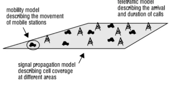
sends and receives phone calls by communicating with a BS on a radio channel. The area which is covered by a BS, i.e. in which a MS can communicate with the BS, is referred to as a cell. The shape of the cell depends on the radio signal propagation. When a call is set up, the MS tries to allocate a free channel from the BS from which it receives the strongest radio signal. If no channel is availa-ble the call is blocked. When a MS finds another BS with better signal strength than the current BS plus a certain margin, it tries to allocate a new channel from that BS to continue the call. This sequence is referred to as a hando-ver. If the signal strength (i.e. link quality) drops below a certain level for an extended period of time and the MS fails to find a better channel, the call is eventually dropped. One goal for the designer of cellular communication sys-tems is to reduce the dropping and blocking probabilities. An abstract model of a cellular communication system can be divided into three sub-models describing the mobility, signal propagation and teletraffic respectively, see Figure 1. This model is, however, not suitable to map directly to a parallel simulation model.
Figure 1. The three submodels of the abstract cellular communication system model
A specific problem in cellular communication systems is that two actors communicating on the same radio chan-nel or on adjacent chanchan-nels can cause calls to be dropped due to interference if not sufficiently geographically sepa-rated. Two methods for allocating radio channels to base stations exist. Most current systems use a Fixed Channel Allocation scheme (FCA), in which channels are statically allocated to base stations so that interference problems are avoided. Better resource utilization can be achieved if base stations can dynamically allocate channels on demand while adhering to certain conditions regarding interference. The latter scheme is referred to as Dynamic Channel Allo-cation (DCA).
In our simulation model each channel is modelled as an LP. There is also an LP which generates new mobile sta-tions when new calls arrive and sends them to the channel selected for the call. The channel LP maintains relevant information on all mobile and base stations which use the channel. This information is sub-divided on a base station basis to MS-BS connections. The signal propagation
char-feq 1 a c --- r x --+ ---=
signal propagation model describing cell coverage at different areas mobility model describing the movement of mobile stations
teletraffic model describing the arrival and duration of calls
acteristics as a function of the geography is maintained in a read only data object available to all LPs.
In the simulation model the mobility of the mobile sta-tions causes the channel objects to schedule events for themselves corresponding to position updates for the mobile stations communicating on the channel. The posi-tion updates are scheduled to occur whenever the mobile station reaches a new position in the signal propagation grid. A position update only modifies part of one MS-BS connection, 20 to 40 bytes on the average, in the state of the LP. At regular time intervals, each 0.5 sec, a MS checks its received signal strength. If it finds a better BS it triggers a handover attempt. In a handover the MS randomly selects a new channel among the available channels, i.e. channels available at adjacent base stations which can provide a suf-ficient signal quality. In particular this causes the LP to communicate with all eligible channels.
The experiments have been performed with an FCA model and a DCA-like model. In all experiments the num-ber of channels has been fixed to 21. Two different areas have been simulated, a small area with 7 base stations and a large area with 67 base stations. Table 1 presents the most important characteristics of the respective models. In our current implementation the state size does not change between the small and large areas.
4. Experimental results
In this section we present the experimental results from applying the state saving mechanisms described in Section 2 to the benchmarks presented in Section 3. The performance measures which we are interested in are: (i) the execution speed compared to copy state saving; and (ii) the memory consumption. The execution speed is pre-sented as the relative execution speed to copy state saving.
In order to better understand the results we also present the checkpoint intervals which the SSS algorithms use and the efficiency defined as the total number of committed events to the total number of events executed (including events which are later rolled back). A state saving/restoration mechanism has a direct impact on the execution time in terms of changing the state saving and state restoration costs. Moreover, this can change the relative speed of dif-ferent LPs which in turn may affect the inherent synchrony of the simulation model, see Section 1. Since this is exploited by the optimistic synchronization it could affect the number of rollbacks in the system which is measured by the efficiency. In the graphs, the algorithms are referred to by the following acronyms:
•CSS, Copy State Saving, Section 2.
•SSS Sx, Sparse State Saving with static checkpoint inter-val x, Section 2.1.1.
•SSS R, Sparse State Saving, Rönngren’s execution time based method, Section 2.1.2.
•SSS M, Sparse State Saving, Rönngren’s memory con-sumption based method, Section 2.1.3.
•SSS F, Sparse State Saving, Fleishmann-Wilsey’s heuris-tic method, Section 2.1.4.
•UISS, User dependent Incremental State Saving, non-transparent ISS method Section 2.2.1.
•TISS, Transparent Incremental State Saving,
Section 2.2.2.
All experimental results have been measured for simula-tions of 5000 seconds of traffic in the simulated systems. This is a sufficiently long period for the simulations to reach a stable behaviour in terms of efficiency and memory consumption. The relative error in the measured values are less than 5%. Performance figures are, primarily, reported for executions on 4 processors. The 2 processor perform-ance figures are only presented in cases where the behav-iour of the state saving mechanisms deviated from the corresponding 4 processor case.
4.1. Expected Performance
From a users perspective it is desirable to have some method to base decisions on how to choose the state saving method which will give the best performance results. In particular, the user has to choose between copy, sparse and incremental state saving. To be able to use the methods proposed in [13] (EQ 4) and [4] (EQ 5) we have measured the following parameters, Table , for the different bench-marks using CSS. For UISS the increment (or location) size is the size of a MS-BS connection, Table 1 (Section 3.1). In the TISS case the average increment size is 4 bytes. Furthermore, the following measured values are necessary to use the method by Cleary et. al. (EQ 5): the
Table 1. Event granularity and state size charac-teristics for the benchmark models
FCA small FCA large DCA small DCA large
Average event execution time, µs
260 750 430 830
State size, bytes 1720 1720 42776 42776 Time to copy a state, µs 140 140 2200 2200 MS-BS connection, bytes 156 156 636 636 Average fraction of state
modified in an event exe-cution
< 1.8 % < 2.3 % < 0.1 % < 0.15 %
Fraction of total execu-tion time spent in state saving when using CSS
~ 35 % ~ 15 % ~ 84 % ~ 72 %
Radio propagation data ~ 0.2Mb ~ 27Mb ~ 0.2Mb ~ 27Mb Minimum memory
requirement: 21 LP states + radio propagation data
time to backup a MS-BS connection in UISS is 45 µs in the FCA case and 76 µs in the DCA case; the time to backup the average increment size 4 bytes in TISS is 15 µs. Based on these measurements and those of Tables 1 and 2, the fol-lowing predictions on the choice between sparse state sav-ing and incremental state savsav-ing are obtained.
The predictions on the largest average fraction of the state updated for which ISS will outperform CSS given by the method of Cleary et. al. [4] (EQ 5) is presented in Table 3. When compared to the figures in Table 1 we see that this method predicts that both TISS and UISS should outperform CSS for all benchmarks with one exception when TISS is used for the large FCA model. The experi-mental results of Section 4.2, Figures 2 through 9, support these results. Palaniswamy and Wilsey’s method [13] (EQ 4) predicts that TISS and UISS will outperform SSS if the number of increments saved in an average event execution is lower than the values in Table 4. The best choice is given by a comparison to the measured number of updates from our experiments also found in Table 4. When compared to the experimental results, Section 4.2, it is evident that this method fails to capture the relation between ISS and SSS correctly. In particular it predicts that the ISS methods should perform better for the FCA models than for the DCA models. The experimental results, Figures 2 through 9, contradicts this theory. In particular, this can be attrib-uted to the fact that the method predicts that ISS performs better for simulations where the ratio of the event execution time to the time to copy a complete state is high. However, the success of ISS depends more on the state size and in particular the fraction of the state updated on average.
4.2. Speed-up and Checkpoint Intervals
One of the primary goals of selecting a state saving method other than CSS is to improve the execution speed. In this section we present the execution speed of the meth-ods described in Section 2 on the benchmarks relative to the execution speed when CSS is used. Furthermore, the checkpoint intervals selected by the SSS methods are pre-sented since these are key factors to asses the performance of these methods.
Figure 2 presents the relative speed of the state saving mechanisms for the small FCA model. For this model the SSS mechanisms perform better than the ISS methods. This is explained by the fact that for the relatively small state sizes of the FCA models the overhead of the ISS mechanisms is higher compared to the overhead of the SSS mechanism. Sparse state saving with a fixed checkpoint interval of 5 results in a reduction of the execution time of more than 30% (corresponding to a relative speed-up of nearly 1.5) compared to CSS. When contrasted to the frac-tion of the total execufrac-tion time spent on state saving using CSS, Table 1, we see that this is a near optimal result. The
a. One MS-BS connection plus 2 integers are saved on aver-age
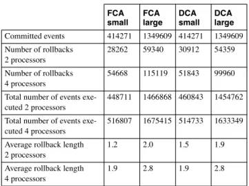
Table 2. Rollback characteristics using CSS exe-cuting on 2 and 4 processors respectively
FCA small FCA large DCA small DCA large Committed events 414271 1349609 414271 1349609 Number of rollbacks 2 processors 28262 59340 30912 54359 Number of rollbacks 4 processors 54668 115119 51843 99960 Total number of events
exe-cuted 2 processors
448711 1466868 460843 1454762 Total number of events
exe-cuted 4 processors
516807 1675415 514733 1633349 Average rollback length
2 processors
1.2 2.0 1.5 1.9
Average rollback length 4 processors
1.9 2.8 1.9 2.8
Table 3. Fraction of the state which can be updated for ISS to outperform copy state saving according to the method by Cleary et. al. [4]
FCA small FCA large DCA small DCA large UISS 2 processors 28% 28% 41% 42% UISS 4 processors 27% 27% 39% 39% TISS 2 processors 2% 2% 2% 2% TISS 4 processors 2% 2% 2% 2%
Table 4. Predictions by Palaniswamy and Wilseys method for ISS to outperform SSS
FCA small FCA large DCA small DCA large
estimatedµinc UISS 2 proc. 6.0 8.0 14.0 13.1 estimatedµinc UISS 4 proc. 7.3 9.1 17.4 15.9 estimated µinc TISS 2 proc. 234 315 2250 2090 estimated µincTISS 4 proc. 285 357 2772 2530 Fraction of state which can
be updated while ISS out-performs SSS
54 - 66 % 73 - 83 % 21 - 26 % 20 - 24 %
TISS average number of increments saved in an event execution
3.9 4.8 6.0 7.4
UISS average number of increments saved in an event executiona
fact that SSS with fixed checkpoint interval in general per-forms best of the SSS methods, Figures 2 to 9, can be explained by the homogeneous nature of the LPs and the communication pattern of the benchmarks.
Figure 2. Speed-up for the small FCA model on 4 processors
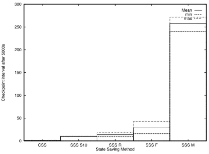
Figure 3 shows the minimal, maximal and average checkpoint intervals selected by the SSS mechanisms.
Figure 3. Checkpoint interval for the small FCA model on 4 processors
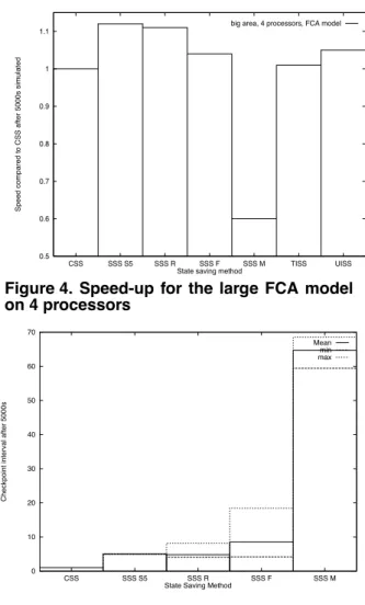
When compared to Figure 2 it is clear that the SSS methods which achieves the best performance in terms of execution speed are those that make the best approxima-tions of the execution speed optimal checkpoint interval. For this model the optimal interval is close to 5. We can also see that the SSS method targeted to reduce the mem-ory consumption, “SSS M”, selects significantly larger checkpoint intervals than the other methods. This is not surprising since larger checkpoint intervals could be expected to give larger reduction of the memory consump-tion. The performance figures for the large FCA model, Figure 4 speed-up and Figure 5 checkpoint interval, further emphasise the results for the SSS methods obtained for the small FCA model, Figures 2 and 3. Figure 5 reveals that
Rönngren’s method, “SSS R”, derives better estimates of the execution time optimal checkpoint interval than the other adaptive SSS algorithms. Fleischmann-Wilsey’s method, “SSS F”, tends to over-estimate the checkpoint interval and also shows a larger variation in the intervals selected. Consequently, Rönngren’s method performs bet-ter than Fleischmann-Wilsey’s, Figure 4. These figures also shows that the high checkpoint intervals selected by the “SSS M” method without regard to the execution time can cause the execution time to increase, Figure 4. This is a consequence of an increased rollback cost in terms of long coast forward phases.
Figure 4. Speed-up for the large FCA model on 4 processors
Figure 5. Checkpoint interval for the large FCA model on 4 processors
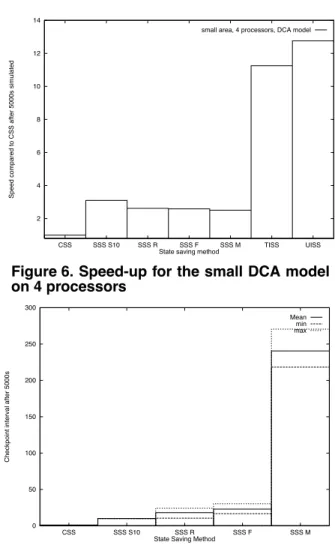
The DCA models features radically different character-istics compared to the FCA models, Table 1. In particular the state size is much larger and the fraction of the state modified in an event execution is much smaller. Intuitively this should favour the ISS methods. The speed-up figures for the small DCA model, Figure 6, clearly indicate that this is the case. The ISS methods outperform the SSS methods by a factor 3 to 4. It is interesting to notice that the
0.8 0.9 1 1.1 1.2 1.3 1.4 1.5 CSS SSS S5 SSS R SSS F SSS M TISS UISS
Speed compared to CSS after 5000s simulated
State saving method
small area, 4 processors, FCA model
0 20 40 60 80 100 120 140 CSS SSS S5 SSS R SSS F SSS M
Checkpoint interval after 5000s
State Saving Method
Mean min max 0.5 0.6 0.7 0.8 0.9 1 1.1 CSS SSS S5 SSS R SSS F SSS M TISS UISS
Speed compared to CSS after 5000s simulated
State saving method
big area, 4 processors, FCA model
0 10 20 30 40 50 60 70 CSS SSS S5 SSS R SSS F SSS M
Checkpoint interval after 5000s
State Saving Method
Mean min max
performance improvement compared to CSS is much larger than what could be attributed only to the reduction of the state saving overhead. As indicated by Table 1, the fraction of the execution time spent on state saving when CSS is used is 84% for this particular model. A complete reduc-tion of this overhead cannot account for more than a 6.25 relative speed-up. Since the efficiency is not significantly affected (compare Figure 13) this has to be attributed to other factors.
Figure 6. Speed-up for the small DCA model on 4 processors
Figure 7. Checkpoint interval for the small DCA model on 4 processors
We believe that this effect can be explained by an improved performance of all layers of the memory system. The large reduction of the memory consumption from the ISS meth-ods could improve performance of the built in memory management schemes of the simulation kernel, the virtual memory system of the operating system and the cache behaviour. In particular, we believe that the cache perform-ance is crucial. Any data item written is moved into the caches, possibly at the expense of some other data being moved out of the cache. For the DCA models the state sizes are so large that saving even a few complete states could evict other, more useful data from the caches. By using ISS
techniques this effect could be reduced. For the SSS mech-anisms it is worth noting that they show similar perform-ance, Figure 6, though the checkpoint intervals differ by more than an order of magnitude, Figure 7.
For the large DCA model, Figures 8 and 9, the perform-ance difference between the SSS mechanisms and the ISS mechanisms is not as pronounced as for the small model, Figure 6. This can be explained by the larger event execu-tion times for this model, Table 1. Furthermore, the maxi-mum speed-up is close to the 5.56 speed-up which could be attributed to a complete reduction of the state saving over-head of 72% when CSS is used. The main difference between the small and the large DCA model is in the size of the signal propagation matrix, which is 0.2Mb for the small model and 27Mb for the large model. Since the cache size is 1Mb on the target computer we can expect cache performance to be worse for the large model while it can be reasonable for the small model if the memory consumption in terms of state saving overhead can be kept low.
Figure 8. Speed-up for the large DCA model on 4 processors
It is interesting to see that the performance difference between the non-transparent, “UISS”, and the transparent, “TISS”, methods for ISS is not very large. Thus we con-clude that for many practical applications transparent ISS is preferable to non-transparent ISS given the drawbacks of the latter, Section 2.2.
Another general tendency which was observed is that the speed-up obtained by the improved state saving mecha-nisms compared to CSS is higher for the same models when the number of processors used is increased. In other words, these methods tend to improve the parallelism. The states are allocated from private memory. Consequently, the improvements cannot be explained by reduced cache coherency problems. However, the reduced memory con-sumption, Figures 10 and 11, could reduce the traffic on the system bus which could make it easier to efficiently send event messages between LPs allocated to different proces-sors improving the parallelism.
2 4 6 8 10 12 14 CSS SSS S10 SSS R SSS F SSS M TISS UISS
Speed compared to CSS after 5000s simulated
State saving method
small area, 4 processors, DCA model
0 50 100 150 200 250 300 CSS SSS S10 SSS R SSS F SSS M
Checkpoint interval after 5000s
State Saving Method
Mean min max 1 2 3 4 5 6 CSS SSS S10 SSS R SSS F SSS M TISS UISS
Speed compared to CSS after 5000s simulated
State saving method
Figure 9. Checkpoint interval for the large DCA model on 4 processors
4.3. Memory consumption
The amount of memory allocated by the system has been measured for simulations of the large FCA and DCA models. Approximations of the minimum memory require-ments for these models are 27.3 Mb and 27.8 Mb respec-tively, Table 1. Thus only memory consumption over these figures are due to state (or event) saving. Figures 10 and 11 depicts the measured memory consumption for these mod-els.
Figure 10. Memory consumption for the large FCA model
The larger memory consumption for the DCA model is a consequence of the larger state sizes. All methods drasti-cally reduce the memory overhead due to state saving. In particular the ISS and the “SSS M” methods perform best for both models. However, the fact that the “SSS M” method can severely degrade the execution speed, Section 4.2, makes it a less attractive
5. Efficiency
The efficiency of a Time Warp system, defined as the ratio of committed events to the total number of executed
events, could potentially be affected by the state saving methods. In general, the investigated state saving methods result in an increased speed in forward execution and a higher state restoration cost in case of rollback. Both these factors could result in a different timing of the delivery of events in the simulation which could affect the efficiency. Figures 12 and 13 depicts the efficiency for simulations of the large FCA and DCA models. For the FCA model there are no significant differences in the efficiency except for the “SSS M”, method. The drastically larger checkpoint intervals of this method makes rollbacks costly. This can cause an LP subject to rollback to lag behind other LPs executing on other processors. The LP lagging behind can in turn cause these LPs to rollback when it resumes for-ward execution.
Figure 11. Memory consumption for the large DCA model
Figure 12. Efficiency for the large FCA model
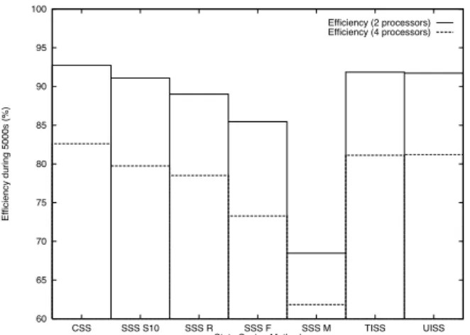
For the DCA model all SSS mechanisms show a degra-dation of the efficiency. In this model the cost to restore a state by copying it is high due to the size of the states. In particular this together with the increased state restoration cost due to the larger checkpoint intervals, Figure 9, is suf-ficient to cause the same type of “lagging behind” behav-iour as the “SSS M” method cause in the FCA model.
0 50 100 150 200 250 300 CSS SSS S10 SSS R SSS F SSS M
Checkpoint interval after 5000s
State Saving Method
Mean min max 28 30 32 34 36 38 40 CSS SSS S5 SSS R SSS F SSS M TISS UISS
Memory Consummed after 5000s (Mb)
State Saving Method
Memory consumption (2 procs)
Memory consumption (4 procs) 30
40 50 60 70
CSS SSS S10 SSS R SSS F SSS M TISS UISS
Memory Consummed after 5000s (Mb)
State Saving Method
Memory consumption (2 procs) Memory consumption (4 procs)
60 65 70 75 80 85 90 95 100 CSS SSS S5 SSS R SSS F SSS M TISS UISS Efficiency during 5000s (%)
State Saving Method
Efficiency (2 processors) Efficiency (4 processors)
The ISS methods show consistently good behaviour in terms of efficiency for both models. In particular the small fractions of the states saved by these methods makes state restoration cost effective which prevents “lagging behind” behaviour.
Figure 13. Efficiency for the large DCA model
6. Conclusions
In this paper we have studied the effect of several state saving mechanisms on the simulations of large, realistic cellular communication systems. Of the investigated adap-tive SSS mechanism the method proposed by Rönngren and Ayani [14] consistently gave the best results. Two methods for incremental state saving have also been stud-ied, one transparent and a more traditional non-transparent method. The experimental results indicate that incremental state saving mechanisms are preferable to SSS when the state sizes are large and only a small fraction of the state is updated in an event execution. Furthermore, the empirical study shows that the cost to achieve transparency for incre-mental state saving is negligible for many practical applica-tions. We believe that transparency is an important aspect of a state saving mechanism as it will help increasing the acceptance and usability of PDES mechanisms based on optimistic synchronization by alleviating the user of the burden of understanding the often intricate underlying exe-cution mechanism.
The performance results indicate that the choice between sparse and incremental state saving mechanisms depends on the characteristics of the simulation model in a way that is often not obvious to the user. Thus, it is useful to have analythical methods to guide such decisions. Two such methods have been investigated. A method by Cleary et. al. [4] to guide selection of incremental state saving compared to ordinary copy state saving gave useful results despite its simplicity. However, we believe that this is a field which merits further investigation.
For future PDES systems based on Time Warp we believe that it is essential that the underlying simulation kernel automatically can select the best state saving
mecha-nism. In particular, different LPs in the same simulation model may exhibit different characteristics which makes a SSS mechanism appropriate for some LPs while others would benefit more from incremental state saving. This emphasises the importance of transparent mechanisms as this is a prerequisite for fully automated methods to select sparse or incremental mechanisms. In this context, our study of analythical methods for such a selection clearly indicates that this is an area which deserves further investi-gation.
7. References
[1] H. Bauer et al., “Reducing Rollback Overhead in Time-Warp Based Distributed Simulation with Optimized Incremental State Saving”, Proceedings of the 26th Annual Simulation Symposium, pages 12-20, March 1993.
[2] Butler R., Lusk, E., “Monitors, messages, and clusters: the p4 parallel programming system”, Parallel Computing, 20, April 1994
[3] D. Bruce, “The Treatment of State in Optimistic Systems”, Pro-ceedings of the 9th Workshop on Parallel and Distributed Simulation (PADS95), pages 40-49, June 1995.
[4] J. Cleary, F. Gomes, B. Unger, X. Zhonge and R. Thudt, “Cost of State Saving & Rollback”, Proceedings of the 8th Workshop on Parallel and Distributed Simulation, Vol. 24, No. 1, pages 94-101, July 1994.
[5] R. Fujimoto, “The Virtual Time Machine”, Proceedings on Par-allel Algorithms and Architectures, pages 199-208, June 1989.
[6] R. Fujimoto, “Time Warp on a Shared Memory Multiproces-sor”, Transactions of the Society for Computer Simulation, Vol. 6, No. 3, pages 211-239, July 1989.
[7] R. Fujimoto, “Parallel Discrete Event Simulation”, Communica-tions of the ACM, Vol. 33, No. 10, pages 30-53, October 1990.
[8] J. Fleischmann and P. A. Wilsey, “Comparative Analysis of Periodic State Saving Techniques in Time Warp Simulators”, Proceedings of the 9th Workshop on Parallel and Distributed Simulation, pages 50-58, June 1995.
[9] D. Jefferson, “Virtual Time”, ACM Transactions on Program-ming Languages and Systems, Vol. 7, No. 3, pages 404-425, July 1985.
[10] Liljenstam, M., Ayani, R., “A Model for Parallel Simulation of Mobile Telecommunication Systems”, To appear in Proceedings of the International Workshop on Modeling Analysis and Simulation of Compu-ter and Telecommunication Systems (MASCOTS), San Jose, CA, Febru-ary, 1996
[11] Y.-B. Lin, B. R. Preiss, W. M. Loucks and E. D. Lasowska, “Selecting the Checkpoint Interval in Time Warp Simulation”, Proceedings of the 7th Workshop om Parallel and Distributed Simulation (PADS93), pages 3-10, May 1993.
[12] J. Montagnat, R. Rönngren and M. Liljenstam, “A technique to implement transparent incremental state saving in Time Warp discrete event simulations”, Department Report, Dept. of Teleinformatics, Royal Institute of Technology, September 1995.
[13] A.C. Palaniswamy and P. A. Wilsey, “An Analythical Compari-son of Periodic Checkpointing and Incremental State Saving”, Proceedings of the 7th Workshop on Parallel and Distributed Simulation, pages 127-134, May 1993.
[14] R. Rönngren and R. Ayani, “Adaptive Checkpointing in Time Warp”, Proceedings of the 8th Workshop on Parallel and Distributed Simu-lation, pages 110-117, July 1994
[15] J. Steinman, “SPEEDES: A Multiple-Synchronization Environ-ment for Parallel Discrete-Event Simulation”, International Journal in Computer Simulation, Vol. 2, No. 3, Pages 251-286, 1992.
[16] J. Steinman, “Incremental State Saving in SPEEDES Using C++”, Proceedings of the 1993 Winter Simulation Conference, pages 687-696, December 1993. 60 65 70 75 80 85 90 95 100 CSS SSS S10 SSS R SSS F SSS M TISS UISS Efficiency during 5000s (%)
State Saving Method
Efficiency (2 processors) Efficiency (4 processors)