Open questions about homogeneous fluid dynamos: the VKS experiment
Texte intégral
Figure
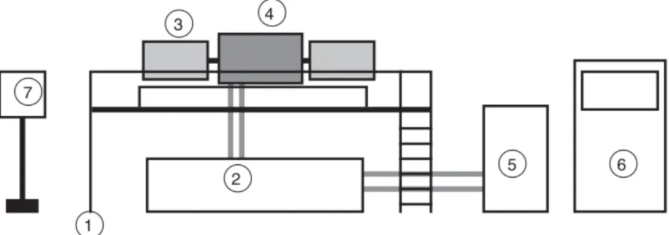
![Fig. 2. Experimental set-up. Poloidal ( a ) and toroidal ( b ) components of the time averaged velocity profile in the counter-rotating von K´ arm´ an flow measured from LDV in a prototype water experiment with dics of 38 cm diameter and curved blades [42]](https://thumb-eu.123doks.com/thumbv2/123doknet/13209377.393145/8.892.143.756.76.436/experimental-poloidal-toroidal-components-averaged-velocity-prototype-experiment.webp)


Documents relatifs
Thus, the twofold aim of the present study was to (i) test whether the systems models used to describe the training response in athletes could be applied in rats and (ii) verify
Our contextualized public transportation game confirms the general relationship between dishonesty in the lab and in the field with some differences with the die task, which
We also test whether it is more effective to introduce crackdowns at an early or later stage of the game, and whether crackdowns should be pre-announced ex ante or not
The low threshold discriminator gives the time reference (figure 6) as long as the delay between the avalanche precursor and the streamer signals is less than 10ns, as
En perspectives, des études supplémentaires intégrant la recherche d’autres mycotoxines (DON, T-2, et HT-2) et l'analyse du potentiel toxique, sont nécessaires
In fact, we were able to conclude the 3-way handshake with 2.2 million hosts on port 179 (vs. Clearly our number is inflated by the fact that we hit not only routers, but also
Two hundred fifty days after casting, the relative humidity in the center of the column reached 85%, and the column was wrapped in plastic to prevent change of its
permeability is relatively high within the fault zone, the overall permeability structure 357. is no higher than that in the lower crust; consequently, because brittle failure
