READ THESE TERMS AND CONDITIONS CAREFULLY BEFORE USING THIS WEBSITE. https://nrc-publications.canada.ca/eng/copyright
Vous avez des questions? Nous pouvons vous aider. Pour communiquer directement avec un auteur, consultez la
première page de la revue dans laquelle son article a été publié afin de trouver ses coordonnées. Si vous n’arrivez pas à les repérer, communiquez avec nous à [email protected].
Questions? Contact the NRC Publications Archive team at
[email protected]. If you wish to email the authors directly, please see the first page of the publication for their contact information.
Archives des publications du CNRC
Access and use of this website and the material on it are subject to the Terms and Conditions set forth at
The IRS Fricke dosimetry system
Olszanski, A.; Klassen, N.; Ross, C. K.; Shortt, K. R.
https://publications-cnrc.canada.ca/fra/droits
L’accès à ce site Web et l’utilisation de son contenu sont assujettis aux conditions présentées dans le site LISEZ CES CONDITIONS ATTENTIVEMENT AVANT D’UTILISER CE SITE WEB.
NRC Publications Record / Notice d'Archives des publications de CNRC: https://nrc-publications.canada.ca/eng/view/object/?id=3e38a08d-312a-4f14-82a9-9f6a4634a90c https://publications-cnrc.canada.ca/fra/voir/objet/?id=3e38a08d-312a-4f14-82a9-9f6a4634a90c
The IRS Fricke
Dosimetry System
A. Olszanski, N. V. Klassen, C. K. Ross and K. R. Shortt
August, 2002
PIRS-0815
Ionizing Radiation Standards
Institute for National Measurement Standards
National Research Council
Ottawa, Ontario, K1A 0R6
Telephone: 613-993-2197
Fax: 613-952-9865
Abstract
This report describes in detail the principal characteristics of the NRC Fricke system. The procedure for making the Fricke solution and a description of the Millipore water system are included. Fricke solutions are irradiated in pancake shaped quartz vials and the readouts are done in Hellma quartz spectrophotometer cuvettes. The cleaning and filling of the vials, the cuvettes, and all other glassware is described since cleanliness is a very important factor in attaining good precision. The absorbance is read using a Varian model Cary 400 UV-Vis spectrophotometer equipped with a high performance R928 photomultiplier tube and a specially designed sample holder. The modifications to the Cary 400 are described in detail. Software, in Application Development Language (ADL), was developed to control the readouts of the Fricke samples. The absorbance readouts of the irradiated samples are discussed, especially as they apply to measurements of absorbed dose (60Co γ-rays) in the range 5-25 Gy. The standard uncertainty on the mean of a set of eight such measurements is normally between 0.05% and 0.15%. Some results showing the stability and reproducibility of the Fricke system are presented. Safety issues associated with the handling and use of the Fricke solution are outlined.
Contents i
1. Introduction 1
2. Cary 400 UV-Vis Spectrophotometer 2
2.1 Factory specifications and design ... 2
2.2 Modifications to the sample compartment and the sample transport... 3
2.3 Light spot position ... 14
2.4 ADL Software ... 17
3. Description of the Fricke System 20 3.1 The physical setup... 20
3.2 Preparation of the dosimeters... 22
3.2.1 Preparation of the Fricke solution ... 22
3.2.2 Filling the vials ... 29
3.3 Irradiations ... 33
4. Spectrophotometric readouts 34 4.1 Filling the cuvettes ... 34
4.2 Absorbance readings ... 35
4.3 Temperature control and nitrogen purging ... 36
4.4 Long and short term consistency and reproducibility... 36
5. Data analysis and absorbed dose evaluation 48 5.1 Water optical density compared with expectations... 48
5.2 Controls and optical density growth compared with expectations ... 51
5.4 Summary of the Fricke analysis ... 55 6 Safety Considerations 59 7 Conclusions 59 8 Acknowledgements 60 9 References 60
List of Figures
Figure 1: Percent transmittance versus distance travelled by the sample transport before modifications (coarse scale). ... 4 Figure 2: Schematic diagram of the sample holder accessory and sample transport accessory... 6 Figure 3: Percent transmittance versus distance travelled by the sample transport before modifications (fine scale) ... 9 Figure 4: Percent transmittance versus distance travelled by the sample holder after modifications (coarse scale). ... 10 Figure 5: Percent transmittance versus distance travelled by the sample holder after modifications (fine scale).. ... 11 Figure 6: Temperature calibration plots of the modified spectrophotometer compartment... 13 Figure 7: Scan to determine the width of the Cary 400 spectrophotometer light spot ... 15 Figure 8: Plot of % transmittance against size of the opening measured from the bottom of slot #1 in the sample holder... 16 Figure 9: Dimensions of the light spot and its position relative to the cuvette ... 18 Figure 10: Photographs of (a) the Fricke vials and (b) the spectrophotometer cuvettes. ... 21
Figure 12: Total organic content of Millipore water over a 5 month period measured with the
Anatel A10 TOC Meter... 26
Figure 13: Effect of the sulfuric acid concentration on the sensitivity of the Fricke solution. ... 30
Figure 14: Effect of the NaCl concentration on the sensitivity of the Fricke solution... 31
Figure 15: Long term zero stability in slot 1 in the Cary 400 spectrophotometer. ... 38
Figure 16: Comparison of zero optical density readings for four sample slots... 39
Figure 17: Slope versus date for the Plastic Phantom Experiment ... 41
Figure 18: Long term stability of all filters (SRM 2031) at 224 nm ... 43
Figure 19: Long term stability of all filters (SRM 2031) at 303 nm ... 44
Figure 20: 30% T Filter short-term stability test over 12 hours... 46
Figure 21: Comparison between 30% T Filter readings taken with the Cary 210 and Cary 400 spectrophotometers... 47
Figure 22: Water absorbance readings in two different slots (1 and 3) taken with the Cary 400 spectrophotometer over 12 h at 224 nm and 303 nm ... 50
Figure 23: Plot of ∆OD vs. dose for a typical experiment ... 57
List of Tables
Table 1: Specifications of the Millipore water... 25Table 2: Expected OD values for water-filled cuvettes. ... 49
1. Introduction
The Fricke dosimeter, also called the ferrous sulfate dosimeter, is one of the most useful chemical dosimeters. It depends on the oxidation of ferrous ions (Fe2+) to ferric ions (Fe3+) by ionizing radiation. The increase in concentration of the ferric ions is measured spectrophotometrically at the optical absorption maxima at 224 nm and 303 nm. The Fricke dosimeter is 96% water (by weight), hence its attenuation of radiation closely resembles that of water. It is usable in the dose range of 5-400 Gy and at dose rates up to 106 Gy/s. For standard photon and electron therapy beams its response is almost independent of beam quality. Its disadvantages include a very high sensitivity to organic impurities that act as scavengers of hydroxyl radicals, ultimately resulting in over-response and the fact that the sensitivity of the system decreases when the oxygen present in the solution is depleted.
This report gives a detailed description of the preparation, materials, instruments, data acquisition and data analysis required for the Fricke dosimetry system at NRC. The dosimeter solution, irradiation vials, readout cuvettes and Cary 400 UV–Visible spectrophotometer are described. Fricke dosimetry is used at NRC for γ-rays, high-energy x-rays and electrons. For precise measurements, the doses delivered to the dosimeters do not exceed 100 Gy and typically range between 5 and 25 Gy. The Cary 400 spectrophotometer is interfaced with a computer. An ADL (Application Development Language) Shell provided by Varian, along with internally developed software, is used for signal processing and absorbance measurements. A detailed
description of both the hardware and the software used to take readings is given in section 2 of this report.
Ultimately, a plot of the net absorbance versus irradiation time (for 60Co) is obtained and the slope of the line is used to calculate the average dose rate to the Fricke solution in a given volume. In the case of irradiations with high energy electrons or x-rays, the dose per monitor unit is determined using the slope of the line of the optical density versus monitor units. With proper care and a state-of-the-art spectrophotometer, the Fricke dosimetry system at NRC is capable of determining the absorbed dose with a typical precision of 0.1% (1σ).
2.
Cary 400 UV-Vis Spectrophotometer
2.1 Factory specifications and design
A high performance Cary 400 UV-Vis spectrophotometer allows accurate optical density measurements. Its design features include a "floating" solid aluminum casting that isolates the optics from external disturbances, an out-of-plane design of the double Littrow monochromator that reduces photometric noise and stray light and produces excellent resolution, and independent nitrogen purging for the sample compartment and monochromator that allows for improved performance in the low UV region where oxygen absorbs. The range of the Cary 400 extends beyond 6 absorbance units. These characteristics make it an excellent instrument for high precision measurements. For maximum performance of the spectrophotometer it is desirable to allow a warm-up time of 2 hours before any absorbance readings are taken. The spectrophotometer has a temperature-controlled sample holder. Peltier devices located around
acts as a heat sink for the excess heat generated by the Peltiers.
2.2 Modifications to the sample compartment and the sample transport
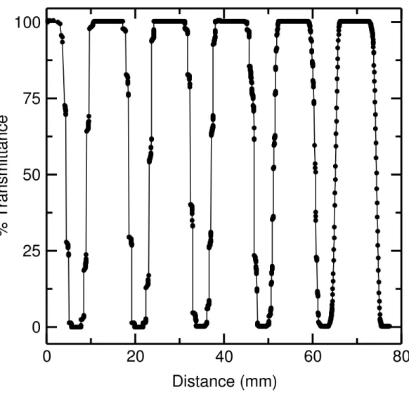
A thermostatted sample holder designed to hold 4 cuvettes with 1, 2 or 4 cm pathlength or other samples (e.g., filters) was built and incorporated into the spectrophotometer. The original holder had 6 slots but only cuvettes with a 1 cm pathlength could be used. Tests determined the positions that give the maximum light transmission through each of the 6 slots in the original holder, and the 4 slots in the modified variable pathlength holder. In order to do the tests, a small program was developed in ADL programming language using “RESETSLIDE” and “SETACC” commands. The UV-Scan software provided by Varian has scans incorporated in it, but the smallest step size is 1 mm, which is far too coarse to position accurately the sample holder. Our ADL program enables the sample transport to move the stepper motor one step at a time, which corresponds to 0.00635 mm. The sample holder position is reset by driving the transport to the home position. At that position, an optical switch is turned on by the moving holder, stopping its motion. In order to test if maximum transmission is attained in the home position, the sample holder assembly was taken out of the spectrophotometer and it was moved backwards inside the assembly in order to scan the first slot. It was not physically possible to move the sample holder far enough to allow the stepwise scan of the entire first slot. Nevertheless, it was moved approx. 2 mm to give a more detailed scan. A detailed 1-step-at-a-time scan of the entire sample holder was done at two different wavelengths, namely 224 nm and 303 nm. The scan at 303 nm is shown in Figure 1 and the one at 224 nm looks essentially the same. It can be seen that the sample transport moves the sample holder in a non-uniform way. It seems that the holder gets
0
20
40
60
80
Distance (mm)
0
25
50
75
100
% Transmittance
% T vs. distance travelled (before modifications)
Figure 1: Detailed scan showing % transmittance as a function of the distance travelled by the sample holder before compartment modifications. Note that the compartment motion is not uniform.
steps. By slot 6 the problem is less severe. As well, the home position (0, 0 in Figure 1) does not correspond to the middle of the opening of slot 1.
Since the reference light passes through 6 slots located at the back of the original sample holder, the light must pass through the middle of both sample and reference slots in double beam measurement mode for the optical density readings to be accurate. Because of this, the reference holder was replaced with a completely open holder, which ensures that the reference light passes only through air (no slots). When the sample holder accessory was changed, it was noted that the reference side holder was connected to the sample side holder only by a piece of flexible tubing through which the cooling liquid flows. This arrangement did not ensure that the relative position of the reference and sample holders remains constant. The connecting tubing was replaced with a much less flexible arrangement to minimize the movement of the reference holder with respect to the sample holder.
When the motion of the sample holder was visually examined, it was clear that the torque produced by the stepper motor was not enough to move the holder step by step. Further examination revealed that the rotor of the motor was spring loaded allowing a fair amount of play in the horizontal movement of the rotor. A schematic diagram of the stepper motor drive that is used to move the holder assembly in the sample compartment is shown in Figure 2. It was noticed that the threaded screw attached to the motor by a flexible bushing turned with considerable resistance. The bearings on which the holder slides and the screw itself were adjusted to reduce the resistance. It was found that the anti-backlash plastic nut had been put on
Sample holder and sample transport diagram
Figure 2: Schematic diagram of the sample holder accessory and sample transport accessory. A dummy holder was placed on the reference side of the sample holder accessory and a Teflon washer was added between the stepper motor casing and the flexible bushing to prevent the spring from compressing and the rotor from moving back inside the motor.
rotor
threaded screw spring
sample holder dummy reference holder
sample holder accessory
horizontal
sample transport accessory
stepper motor casing
backlash plastic nut Teflon washer
flexible bushing
to allow the screw to move smoothly. It was also noted that the sample holder could move about 0.5 mm in the vertical direction on the horizontal bearings. This is not a problem because vertical play in the bearings will not significantly influence horizontal motion.
The torque issue was also investigated. The same drive used to power the sample transport accessory is used to power another accessory with a motor requiring no more than 4 V. The drive was found to put out 4 V, while the motor driving the sample transport is rated for 12 V. An arm was attached to the motor shaft to measure the torque produced. The torque was only ¼ of the torque that the motor should produce. There was also no holding torque produced by the motor, but this is not critical since we are moving the sample compartment horizontally so a holding torque is not necessary.
The electronics of the sample transport drive was modified to give 12 V to the stepper motor coils. This produced a lot more torque and when the sample transport was put back together no slipping was observed. However, when a scan was taken, the problem of missed steps still persisted in the middle of the scan. There was a substantial improvement in compartment motion at the beginning and the end of the scan. Since there was now considerable enhancement in the torque and the sample transport bearings were now properly aligned, other options were investigated.
Periodic movement of the sample transport, and then no movement at all, suggest that there is a force building up as the motor turns, which then is released. Closer observation led to the conclusion that the spring at the end of the rotor inside the motor assembly is compressed as the rotor turns. In other words, it is easier to move the rotor inside the motor inwards than it is to
move the sample transport outwards. This can be easily seen when looking at the sloped part of the scan. A zoomed-in version of the downward slope of the 303 nm scan before modifications is shown in Figure 3. It shows that for approximately 10 steps of the motor there is no change in % transmittance, so the sample holder is not moving. After 10 steps the sample holder jumps 10 steps forward, and then the cycle is repeated. These data suggest that after 10 steps of the rotor there is enough potential energy stored in the spring that when the motor tries to move the sample transport accessory by 1 step, the torque produced combined with the energy stored in the spring results in forward motion of the sample holder (approximately 11 steps). Putting a Teflon washer on the motor shaft and clipping it in place rectified this problem. This arrangement ensures that there is no horizontal play in the rotor movement. The trade off is that it introduces extra friction when the rotor turns, because now it not only has to move the compartment but also the washer that is in contact with the motor wall. The increased torque allows the motor to handle the load. When all the modifications were completed, new scans were done of % transmission vs. number of steps. Figure 4 shows one of these plots at 303 nm. Figure 5 is a zoomed-in version of 303 nm data from Figure 4. There is no periodic motion observed in the movement of the sample transport. The one step at-a-time motion is very reliable.
The original sample holder accommodated six 10 mm path-length cuvettes on the sample side and six 10 mm path-length cuvettes on the reference side. This design was modified and a new variable path-length (10, 20, 40 mm) cuvette holder was made. It replaced the old holder on the sample side while the reference side cuvette holder was replaced with an “open” dummy. Since the new sample holder is more massive than the original one, its temperature control had to be calibrated. The calibration was done by taping a thermocouple to the sample holder wall with
3.0
3.5
4.0
4.5
5.0
5.5
6.0
Distance (mm)
0
25
50
75
100
% Transmittance
% T vs. distance travelled (before modifications)
Expanded scale
Figure 3: Measured % transmittance vs. distance travelled by the sample transport before modifications. Periodic jumps of approximately 10 steps are evident.
0
20
40
60
80
Distance (mm)
0
25
50
75
100
% Transmittance
% T vs. distance travelled (after modifications)
Figure 4: Measured % transmittance as a function of the distance travelled by the sample holder after modifications to the drive system. Smooth motion was established after the changes to the drive were implemented.
3.0
3.5
4.0
4.5
5.0
5.5
6.0
Distance (mm)
0
25
50
75
100
% Transmittance
% T vs. distance travelled (after modifications)
Expanded scale
Figure 5: Percent transmittance against distance travelled by the compartment zoomed in to 3.0 to 6.0 mm. The motion of the compartment is smooth.
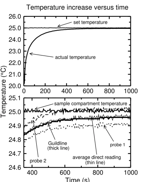
insulating tape and reading its output with a digital reader, Model 871A (Omega Engineering Inc.). The thermocouple plus the reader was calibrated to 0.1°C using a 9540 Digital Platinum Resistance Thermometer (Guildline). This device (which we will refer to in the rest of this report as the “Guildline thermometer”) has been calibrated against NRC temperature standards to 0.03°C. The sample holder temperature was measured from 10°C to 25°C. The potentiometers (slope and intercept) on the Cary circuit board for reading the temperature were then adjusted until the temperature displayed on the Model 871A and by the software matched over the entire temperature range to ± 0.1°C. The temperature calibration of the internal probe was then tested at 25°C by inserting a water-filled 40 mm path-length cuvette into a slot and inserting two external platinum resistance probes and the Guildline thermometer into the water in the cuvette. Measurements of the temperature were then recorded at 5 s intervals for 1000 s. The recorded values included the sample compartment temperature, the set temperature, and the temperatures of both external probes and the reading of the Guildline thermometer. The temperature calibration plot for slot 1 is shown in Figure 6. The average of the readings of the two external probes coincides with the reading of the Guildline thermometer. The set temperature is 0.03°C higher than the water temperature. All other slots were tested in the same way and the average temperature of the solution in the cuvettes in all slots is the same as the temperature read by the Guildline thermometer within 0.05°C. In all cases the actual temperature is lower than the one the sample holder was set to by 0.03 ± 0.02°C.
400
600
800
1000
Time (s)
24.6
24.7
24.8
24.9
25.0
25.1
0
200
400
600
800
1000
20.0
21.0
22.0
23.0
24.0
25.0
26.0
Temperature (°C)
Temperature increase versus time
Guildline probe 1 set temperature
actual temperature
probe 2 average direct reading (thick line)
(thin line)
sample compartment temperature
Figure 6: Measured temperatures within the new spectrophotometer compartment. It takes approximately 5 minutes from the insertion of the cuvette into the compartment for the temperature of the solution to be within 0.2°C of the setpoint. The lower pane is a more detailed view of a portion of the upper pane.
2.3 Light spot position
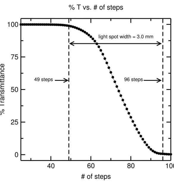
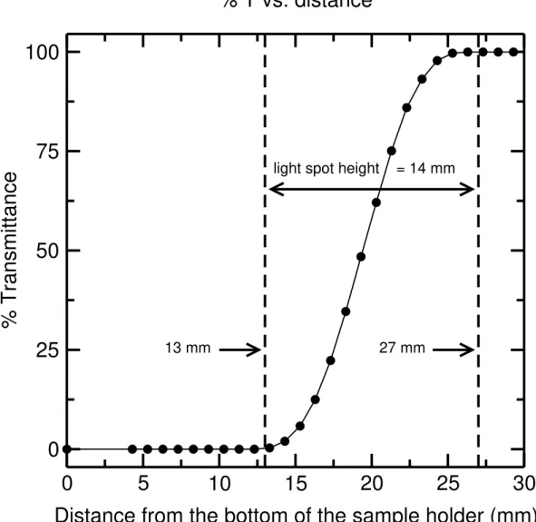
The light spot position within each of the four slots was investigated to ensure that the light beam passes through the center of each slot. It is preferred that there is a 2-3 mm gap between the light spot edges and the top and bottom of the slot. The width of the light beam was determined by scanning across the empty sample holder. The number of steps taken for the light intensity passing through the slot to go from 0 to 100 % transmittance multiplied by the distance travelled by the holder per step equals the width of the light spot (i.e., 47 × 0.0635 = 3.0 mm). This result is shown in Figure 7. With the wavelength set to 500 nm, the width of the light spot was measured with a micrometer to be 3.0 mm. Next, a metal strip was put in place to obstruct the light and moved upwards inside one of the slots in 0.1 mm increments. The position of the strip at which the % T (transmittance) rose above zero defined the bottom edge of the light beam with respect to the bottom of the slot, and the position of the strip at which % T became equal to 100 defined the top edge of the light beam. This is shown in Figure 8.
The distance that the compartment travels per step is quoted by the Cary manual to be 0.06349 mm. This distance was also measured by moving the compartment by a given number of steps and measuring the distance it travelled with a micrometer. In order to improve accuracy, two different measurements were done with different reference points. It was found that the distance by which the compartment moves per step equals 0.002500 inches. This suggests that the screw thread is based on the British measurement system, not the metric one. Since the
40
60
80
100
# of steps
0
25
50
75
100
% Transmittance
% T vs. # of steps
light spot width = 3.0 mm
49 steps 96 steps
Figure 7: Scan across slot 1 to determine the width of the Cary 400 spectrophotometer light spot. 47 steps were required for the edge of the slot to cross the light beam. Each step is 0.0635 mm long and so the width of the light spot is 0.0635 A 47 = 3.0 mm. This value agrees with a direct measurement within ± 0.1 mm.
0
5
10
15
20
25
30
Distance from the bottom of the sample holder (mm)
0
25
50
75
100
% Transmittance
% T vs. distance
light spot height = 14 mm
13 mm 27 mm
Figure 8: Plot of % transmittance against size of the opening measured from the bottom of slot #1 in the sample holder. The first nonzero reading occurs at 13 mm opening size, and the 100 % transmittance is achieved at 27 mm. Therefore the light spot size in the sample holder is 14 mm long and its bottom edge is 13 mm from the bottom of the holder.
we measure 1 step = 0.002500 inch (i.e., 0.06352 mm) compared to 0.06349 mm found in the Cary 400 User Manual, a difference of 0.05 %. We conclude that the distance travelled by the compartment per step is 0.06350 ± 0.00002 mm. Figure 9 locates the light spot in the first slot in the modified sample holder. The units are mm and the uncertainties are ± 0.1 mm.
2.4 ADL Software
In order to use the variable-path-length cuvette holder, software was developed to handle data acquisition. It is based on the ADL Shell provided by Varian and it uses the Application Development Language (ADL) to perform functions necessary for data collection. The software application allows the user to set the readout parameters such as the spectral band width (1.5 nm), averaging time (2 s), number of reads (5) and wait time between reads (2 s) (the values in brackets are those used for a typical experiment). The "averaging time" sets the signal averaging interval used during data acquisition. The higher the value chosen, the more precise the result because the uncertainty due to the dark current is reduced. The number of reads represents the number of replicate readings taken of each sample, and the waiting time between the reads sets the pause interval between each replicate.
The new sample holder has four slots. During a typical experiment, slots 1 and 3 contain the samples to be read, slot 2 is left empty and slot 4 contains a standard absorbance filter. Absorbance readings at the slots containing the samples are taken four times (i.e., 4 x 5
Figure 9: Dimensions of the light spot and its position within slot #1 of the sample holder. All values are given in mm.
time before a sample measurement is taken to verify the zero. If the zero has changed, the most recent value is subtracted from the subsequent sample absorbance readings. All readings are averaged and the final zero, sample one, sample two and filter readings are reported. The software has a built in waiting time of 5 minutes for the temperature equilibrium to be reached between the time of insertion of the cuvettes into the sample slots and commencement of the readings. During the waiting time, the instrument is set so that the light beam passes through the empty slot in order to minimize the possibility of an increase in absorbance of the samples due to oxidation of the Fricke solution in the cuvettes by the UV light. Typically all readouts are taken at a temperature of 25°C " 0.1°C and at 224 nm and 303 nm. The readings at 224 nm are taken before the ones at 303 nm because the extinction coefficient is less temperature sensitive at 224 nm than that at 303 nm. Every time the spectrophotometer is turned on, a wavelength calibration and %T calibration are performed automatically. The wavelength scale of the spectrophotometer can also be checked manually in the “Validate” part of the Cary 400 software package. All absorbance readings are taken in the double beam mode with the reference beam passing through air. Before the samples are analyzed, a text file is created in which vial numbers, irradiation times, irradiation and readout temperatures and absorbance readings are recorded. The software also allows for the data to be printed. The sample compartment temperature is taken to be the readout temperature. A command asking for a direct measurement of the temperature of the solution in a cuvette is incorporated in the software. Typically the difference between the sample compartment temperature and the cuvette temperature is less than 0.1°C.
3.
Description of the Fricke System
3.1 The physical setup
Currently the Fricke system setup at NRC consists of:
• 13 pancake-shaped quartz vials with an internal diameter of 29 mm, internal width of 7 mm and 1 mm thick walls and Teflon stoppers individually fitted to the vials (Figure 10(a))
• Round Lucite holders used to keep the vials in an upright position (Figure 10(a))
• Quartz cuvettes (Hellma Canada Ltd.) with path lengths of 1, 2 and 4 cm and Teflon cuvette covers (Figure 10(b))
• The chemicals used to make the dosimeter solution:
− Ferrous ammonium sulfate hexahydrate [(NH4)2Fe(SO4)2⋅6H2O] (99.997%,
Ultrapure) (Aldrich Chemical Co.)
− Sodium chloride [NaCl] (100.00%, Ultrex grade) (J T Baker Chemical Company) − Sulfuric acid [H2SO4] (95.5%, Ultrex II grade) (J T Baker Chemical Company)
• Sulfuric acid [H2SO4] (96% acid, Analyzed grade) (J T Baker Chemical Company) used
for cleaning glassware • 2000 cm3
quartz flask with quartz stopper used to prepare and store the Fricke solution • Water powered Bernoulli suction pump
• Two electronic scales, Mettler AE 163 (range 30 g, divisions 0.1 mg) and Scientech 5500 (range 5.0 kg, divisions 0.1 g)
Fricke vials and spectrophotometer cuvettes
Figure 10: Photographs of (a) the Fricke vials and (b) the spectrophotometer cuvettes.
vial Teflon stopper Lucite holder Teflon covers cuvettes
(a)
(b)
• Millipore water purifying system
• Laminar flow hood (Cleanline Laminar Flowhood Equipment)
• Cary 400 UV-Vis spectrophotometer with temperature control accessory and variable path-length cuvette holder
• Water I system (Figure 11(a))
• Computer for data acquisition and analysis
• Pipette cleaning system and Kimble 72050 disposable pipettes (Figure 11(b))
• Various accessories: e.g., lint-free Kimwipes, squeeze bottle, spatula, tweezers, separatory funnel, 5-10 ml rubber bulb (pipette filler)
• NIST SRM-2031 metal on quartz standard absorption filters (10% T, 30% T, 90% T) 3.2 Preparation of the dosimeters
3.2.1 Preparation of the Fricke solution
Only high purity ingredients are used to make the Fricke solution at NRC. Water constitutes 96 % of the Fricke solution by weight, hence its purity is important. High purity water at NRC is currently obtained using the Millipore water system (Millipore Corporation). It consists of two units, a Milli-RO 10 Plus and a Milli-Q UV Plus. The Milli-RO 10 Plus reverse osmosis purifier removes more than 90% of the ionic impurities. It has columns to remove four main types of contaminants, namely monovalent ions, polyvalent ions, dissolved organics and other particles
Water I system and pipette cleaning system
Figure 11: Photographs of (a) the Water I system and (b) the pipette cleaning system. The water I system water compartment is filled with Millipore water from the top.
disposable pipette water compartment
Teflon/plastic water/acid inlet pipettes electric pump electronic display water/acid outlet pipette holder
(b)
(a)
and microorganisms. Water from the Milli-RO unit is stored in a 60 L reservoir (Millipore TANK PE0 60). The Milli-Q UV Plus provides the final treatment to the water. A QPAK purification pack eliminates the dead water volume. It contains activated carbon to remove dissolved organics and nuclear grade ion exchange resins to “polish” the final product. A UV lamp oxidizes organic substances and destroys bacteria The final product passes through a Millipak 40 Filter (0.22 µm) just before it is dispensed.
The final water quality should have the specifications listed in Table 1 as stated by the Millipore manual. Total organic carbon is measured on a day-to-day basis with an Anatel A10 TOC monitor (resolution of 1 ppb) and the results are shown in Figure 12. The total organic content in the Millipore water has been consistently at a value of 3 ppb. Based on the good precision of the experiments, the Millipore Water System is routinely used at NRC to provide high purity water for the Fricke solution as well as for equipment cleaning purposes.
The ferrous ammonium sulfate and sodium chloride are stored, tightly sealed and wrapped in aluminum foil to avoid contamination and limit light exposure, in a sealed glass dessicator. The dessicator contains silica gel to absorb moisture. Sulfuric acid is stored in a plastic bottle in the laminar flow hood.
The procedure to make Fricke solution consists of the following steps:
1. Rinse a 2L quartz flask five times and fill it approximately ¾ full (1500g) using Millipore water.
Specification Value*
Resistivity 18.2 Megohm-cm
Total Organic Carbon (TOC) ≤ 5 ppb Particles ≥ 0.22 µm < 1/ml Total dissolved solids < 10 ppb
Silicates < 0.1 ppb Heavy metals ≤ 0.1 ppb
Microorganisms ≤ 1 cfu/mL [cfu = colony forming units]
Table 1: Specifications of the Millipore water as stated by the Millipore Users Manual. * 1 ppb is defined as 1 g of impurity per billion g of water
Apr
May
Jun
Jul
Aug
Month
0
1
2
3
4
5
TOC (ppb)
Millipore TOC vs. Date
Figure 12: Total organic content of Millipore water over a 5 month period in 2002 measured with the Anatel A10 TOC Meter. The resolution of the Anatel is 1 ppb.
dispense the acid to the flask is rinsed five times with the acid before use. If a different assay of the acid is used, Equation (1) can be used to calculate the weight of the acid to be added. 1 0.4[ ] 2[ ] 98.08[ ] 100 [ ] % M L g mol mass g acid − ⋅ ⋅ ⋅ ⋅ = (1)
3. It is a standard practice to pre-irradiate the water-acid mixture to approximately 10 Gy to eliminate non-linearity in the slope at lower doses, resulting from impurities in the acid. We have shown that pre-irradiation changes the sensitivity of the Fricke solution by less than 0.1 % (Klassen et al 1999).
4. Add 0.784 g of ferrous ammonium sulfate hexahydrate.
5. Add 0.1169 g of sodium chloride to reduce the effects of trace organic impurities in the solution.
6. Add Millipore water to reach a final mass of the solution of 2043.4 g.
7. Air-saturate the resulting Fricke solution by swirling it around in the flask, and opening the stopper periodically to let air in.
8. Cover the dosimeter solution with a stopper and store it away from natural and artificial light sources.
Ferrous ammonium sulfate and sodium chloride are weighed using a Mettler Balance model AE163. The balance is calibrated prior to each use and the calibration is checked with
standard 200 g and 500 g weights. The steps involved in the balance calibration are outlined below:
1. Remove all objects from the balance pan. 2. Close the sliding windows.
3. Press control bar until “CAL” is displayed in order to set the balance to the calibration mode.
4. Release control bar (“CAL----” will appear in the display).
5. As soon as “CAL 100” appears (the 100 blinks), slowly move the calibration lever towards the rear. First “Cal ----” appears, then “100.0000”. When the display “Cal 0” appears (0 blinks), move the lever back to the original position, then wait until the display changes to “----” followed by “0.0000”. The balance is now calibrated.
The sulfuric acid and Fricke solution are weighed using a Scientech 5500 balance. The concentrations present in the final dosimetric solution are: 4.0 A 10-1 mol ⋅ L-1
sulfuric acid, 1.00 A 10-3 mol ⋅ L-1
ferrous ammonium sulfate, and 1.00 A 10-3 mol ⋅ L-1 sodium chloride. The amounts of constituents added are usually accurate to 0.05%. However, it has been shown that small deviations from the set amount do not significantly alter the results.
To test the influence of the sulfuric acid concentration on the sensitivity of the Fricke solution, a Plastic Phantom Experiment (see section 4.4) was done in which the amount of sulfuric acid in the irradiated Fricke solution was varied. Eight vials were irradiated at multiples of 35 minutes. Two vials were irradiated for each time duration. The experiment was done once with approximately 0.41 M acid, and once with approximately 0.37 M acid. These results were
was obtained and corrected to the reference date for both experiments. The results of varying the acid concentrations in the Fricke solution are shown in Figure 13. The experiment in which the acid concentration was 0.37 M gave the same slope as that obtained in the experiment with the standard acid concentration (0.4 M). The experiment in which the concentration of the acid was 0.41 M showed an approximately 0.4% smaller slope. Therefore, more detailed experiments are necessary to draw a concrete conclusion about the acid concentration effect on the sensitivity of the Fricke solution. Allen at al (Allen et al 1957) showed that the Fe3+ yield is independent of the acid concentration in the range 0.25 - 0.4 M. His result does not contradict our experiments but for acid concentrations greater than 0.4 M more data is necessary.
A variation in NaCl concentration has been investigated by Cottens (Cottens 1979-1980). He showed that the sensitivity of the Fricke dosimeter is only slightly dependent on NaCl concentration. His data are shown in Figure 14 and indicate that changing the NaCl concentration by ± 5% only changes the Fricke sensitivity by ± 0.01%.
3.2.2 Filling the vials
The irradiations are done in pancake shaped quartz vials. Each vial has an opening for filling and emptying. The opening is closed snugly with a Teflon stopper. The vials are filled with the Millipore water and stored in the laminar flow-hood until they are ready for use. At that point they are sequentially rinsed five times with the Millipore water. A Water I system (Gelman
0.36
0.38
0.40
0.42
0.44
Acid concentration (mol · L
-1)
0.0378
0.0379
0.0380
0.0381
0.0382
0.0383
Slope
Slope values for Plastic Phantom Experiment
versus acid concentration
0.0
0.1
0.2
0.3
0.4
0.5
0.6
NaCl concentration (g · L
-1)
0.984
0.986
0.988
0.990
0.992
0.994
0.996
0.998
1.000
G/G
0G/G
0vs. NaCl concentration
NRC value
Figure 14: Effect of the NaCl concentration on the sensitivity of the Fricke solution (Cottens 1979-1980). A variation of ± 5% in the NaCl concentration changes G/G0 by ± 0.01%.
Sciences) is used to dispense the water into the vials through the disposable pipettes. The Water I system consists of a water compartment, a purifying capsule (Barnstead-Thermolyne), and a pump used to circulate the water through the system. The purifying capsule inside the system is changed at least once a year. The Water I system is not used for water purification purposes but only to adequately maintain the purity of the Millipore water and to dispense it for rinsing vials. A polyethylene tube, attached to the Bernoulli suction pump is used to suck the water out of each vial. After the fifth rinse, the Millipore water is not taken out of the vials. They are capped with the Teflon stoppers, dried with Kimwipes and placed in the laminar flow-hood. Prior to use, the pipettes are cleaned with concentrated sulfuric acid (J.T. Baker Analyzed Grade). The acid is circulated through the inside of the pipettes for approximately 4 h using a custom-built quartz/Teflon circulating system (see Figure 11(b)). Next, the pipettes are rinsed with circulating Millipore water five times in the same system (each rinse takes approximately 30 min.). Lastly, they are dried with Ultra-high purity nitrogen under a heat lamp for approximately 2 hrs.
A clean Pyrex separatory funnel is used to transfer the stock Fricke solution to the vials. The funnel, along with the stand and stoppers, is weighed before being used. Its mass is recorded and compared with previous experiments. Weighing the funnel checks that it is clean and dry. The funnel and the stoppers are then rinsed five times with the Fricke solution. The funnel is then filled with the solution that will be used to fill the vials. Transfer of the stock solution to the vials takes place in the controlled environment of the laminar flow hood. All vials are sequentially rinsed with stock solution five times. The rinsing is done by half-filling each vial, capping it with a stopper and shaking it vigorously for a few seconds. The stock solution is then removed from the vial by means of the water aspirator. Once all the vials have been rinsed five times with
sealed with the Teflon stoppers. After being used, the separatory funnel and stoppers are rinsed five times with the Millipore water and left to dry in the laminar flow hood. The process of cleaning and filling of the vials typically takes between 3 to 4 hours so it is usually done a day prior to irradiations. The vials are stored overnight in the upright position, in the dark in the laminar flow hood. After a few hours, a small air bubble appears inside each vial. This probably happens due to an imperfect seal between the vial and the stopper. We believe that this does not influence the amount of Fe3+ produced by irradiation since the bubble corresponds to less than 0.1 % of the volume of the vial (Macfarlane et al ).
3.3 Irradiations
Irradiations are typically done using 60Co γ-rays from the Eldorado 6 (MDS Nordion) irradiator for which the vials are usually irradiated in a water phantom or the Theratron Junior (Atomic Energy of Canada Ltd) irradiator for which the vials are usually positioned in a plastic phantom which is fastened to the head of the irradiator (the Plastic Phantom Experiment).
Normally two sets of four doses are given in random order and four vials are kept as controls. The vials are placed in the radiation field in a reproducible position (usually ± 0.1 mm). The vials are placed upright to minimize the possibility of the solution coming out of the vial. During irradiations the vials are surrounded by water or water equivalent material to ensure electronic equilibrium conditions. The advantage of having a vial in water is that the irradiation temperature can be easily controlled but there is a risk of water from the surroundings entering the vial and contaminating the irradiated solution. To minimize that risk, an O-ring is put around the stopper that has been inserted into the vial. In the case of solid water equivalent material, the
risk of contamination is eliminated and the temperature of the air space in the vial position is taken as the irradiation temperature. The irradiation temperature at the vial position is measured before each vial is irradiated. Each vial is given 5 to 15 minutes to reach the temperature of the surroundings before the irradiation begins. Typical doses given to the vials range between 5 and 25 Gy. The irradiation times are recorded to ± 1 ms. After the irradiation is complete, the irradiated vial is dried if necessary and placed in an up-right position until it is read.
4. Spectrophotometric
readouts
4.1 Filling the cuvettes
Depending on the doses given to the vials, 1, 2 or 4 cm path length cuvettes can be used. The choice between different cuvettes is usually made such that the optical density at 303 nm will be between 0.1 and 0.5. The cuvettes are stored in the laminar flow hood in a covered beaker filled with Millipore water. The cuvettes are rinsed 5 times with the Millipore water before being used. They are also scrubbed with a wet Q-tip inside and out after the second rinse. They are then dried with the aspirator in the laminar flow hood. Clean disposable Pasteur pipettes are used for dispensing the irradiated solution from the vials to the cuvettes. The pipette cleaning process has been described. The solution to be read is transferred with a pipette from the vial to the first cuvette using the rubber bulb. The transfer process consists of sucking some of the solution up into the pipette and wetting its walls. This solution is then discarded. Then, more of the solution is sucked into the pipette and transferred to the cuvette. It is swished around in the cuvette so that all interior cuvette walls are wetted. The solution is then sucked out using the aspirator but the cuvette is not dried. Lastly, the same pipette is used to transfer the remaining solution from the vial to the cuvette that is then capped with a Teflon cover, which has been rinsed with the
pipette. The two cuvettes are usually filled with solution that comes from two different vials irradiated to the same dose.
4.2 Absorbance readings
The optical density is measured using the Cary 400 UV-Vis spectrophotometer. In this instrument, the light is analyzed before it passes through the sample. This reduces photo-oxidation of the ferrous ions because only the desired wavelength of light passes through the sample. The sample transport accessory provided by Varian has been modified (as described in Section 2.2) to hold the 1, 2 and 4 cm path length cuvettes. The sample holder has four cuvette slots, the 1st and 3rd are used for the samples to be measured, the 2nd is left empty to verify zero during absorbance measurements and the 4th holds a metal-on-quartz filter (SRM – 2031) (NIST) to verify the stability of the spectrophotometer during absorbance measurements. The spectrophotometer is allowed 2 h of warm-up time before any absorbance readings are taken. At the beginning of every experiment both cuvettes are filled with Millipore water and read. This is a check of cleanliness of the pipettes, cuvettes and the water itself. It also serves the purpose of ensuring that the spectrophotometer is operating properly. Next the control solution is read in both cuvettes. Then the two cuvettes are filled with the solution from two different vials that have been irradiated to the same dose. The absorbance readings for the two different samples should agree with each other. If not, at least one of the samples or the cuvettes has been contaminated. After all the irradiated samples have been read, another control reading is taken and the readout process is ended with another water reading. All samples are read at 224 nm and then at 303 nm. The readout process of one sample takes approximately 25 minutes. The
sequence in which the irradiated samples are read is randomized as to dose. The same two cuvettes are used to read all the samples, and a given cuvette is always placed in the same slot in the sample compartment. All readouts are done using the ADL software described in section 2.3. The readout result consists of two independent sets of data, one from each of the cuvettes and two control readings for each set.
4.3 Temperature control and nitrogen purging
The spectrophotometer is connected to the temperature accessory provided by Varian. This allows the temperature of the cuvette holder to be controlled to ± 0.05°C (calibration is described in section 2.2) during the readout. UHP nitrogen is used to purge the sample compartment (15 cm3/s) and the optics compartment (100 cm3/s). Every sample is allowed 5 minutes to equilibrate after being placed in the cuvette holder to ensure that the readout temperature is as close to 25°C as possible. After each readout has finished, a temperature probe can be inserted into the solution in each of the cuvettes and the temperature can be measured directly. Historically, the actual readout temperature and the sample compartment temperature agree to ± 0.1°C and so the direct temperature measurement is not necessary. Temperature probes, capable of an accuracy of about ± 0.05 °C, are used to measure the readout temperature. They have been calibrated using the Guildline thermometer.
4.4 Long and short term consistency and reproducibility
The long term stability of the zero reading was investigated in slot 1 by zeroing the spectrophotometer and then taking multiple measurements of % T at 10 s intervals and looking for drifts. The results are shown in Figure 15. Over a 16 h period, % T decreased by 0.03%. The
experiment it is assumed that all 4 slots give the same readings it is important to check the zero stability from one to another. The spectrophotometer was zeroed in slot 2 then repeated absorbance measurements were taken in all slots sequentially. The results are shown in Figure 16. Slots 1 and 4 seem to be reading higher than slots 2 and 3 by 0.0001 odu (optical density units). This difference is not fully understood but it might be due to reflections of the light at the edges of the compartment on the reference side. If that is the case, the light reflecting off the edge of the reference slot adds to the signal on the reference side, increasing the apparent absorbance on the sample side.
The Theratron Junior γ-ray source is used to check the quality of the freshly made Fricke solution, and to check the reproducibility and consistency of the spectrophotometer readings over a long period of time (Plastic Phantom Experiment). The irradiations are done in a Lucite phantom attached to the head of the source. The Lucite phantom is constructed from 9 cylindrically shaped Lucite blocks of different thicknesses with smooth outside surfaces, held together by 3 plastic pins. The face of the phantom to be positioned closest to the source provides a buildup layer of 1.5 mm. It has a slot through it into which a removable piece of Lucite slides. The removable slide has a hole in the middle to hold the vial during the irradiation. A threaded hole in the bottom of the slide, with a nylon screw, is used to hold the vial in place. The outer dimensions of the phantom are: diameter 190 mm, thickness 120 mm. The phantom is attached to the head of the irradiator approximately 30 minutes before the first irradiation to allow the temperature of the Lucite to equilibrate with the surroundings. The numbered vials, in random
0
2
4
6
8
10
12
14
16
Time [h]
99.96
99.97
99.98
99.99
100.00
% Transmittance
Long term zero drift in the Cary 400
spectrophotometer measured in Slot 1
100.01
Figure 15: Long term zero stability in slot 1 in the Cary 400 spectrophotometer. Percent transmittance decreased by approximately 0.03% after 16 h. The readings were taken at 10 s intervals with nitrogen purging. The spectrophotometer was allowed a warm up time of 2 h.
0
60
120
180
240
Time (min)
-5
0
5
10
15
20
Optical density (×10
5)
Zero reading comparison between different slots
slot 1
slot 4
slot 2
slot 3
Figure 16: Comparison of zero optical density readings for four sample slots. Slots #1 and #4 read higher than slot #2 and #3 by 0.0001 odu. This small effect might be due to the fact that the reference light spot is close to the edges of the compartment on the reference side.
order, are positioned in the slide for irradiations. The front face of the vial is co-planar with the front surface of the slide. The nylon screw on the bottom of the slide is tightened to fix the vial’s position. The slide is placed in the phantom with its ends flush with the circumference of the phantom and with the vial in an upright position. This prevents leaking of the solution from the vial during the irradiation. The vial is left inside the phantom for five minutes to allow thermal equilibrium between the vial and the phantom. The maximum field size of the irradiator is used when irradiating the vials. After completion of the irradiation, the slide is removed and a thermometer is put in its place. The temperature it reads is recorded as the irradiation temperature. The thermometer used has divisions of 0.1°C and it has been calibrated using the Guildline thermometer. The irradiation times are chosen so that the doses are equally spaced from 5 to 25 Gy. After the irradiation, the vial is removed from the slide and placed in the laminar flow-hood in the upright position. Typically 8 irradiations are done, at 4 different doses (Section 4.1). Two to four additional vials are kept as controls. The irradiation times are randomized to reduce the possibility of systematic errors resulting from the fluctuations of the temperature during the course of the irradiations.
The slope of the measured ∆OD versus irradiation time is adjusted to a reference date using a half-life of 1925.02 days for 60Co. The resulting slopes over a sixteen year period are shown in Figure 17. The last point in Figure 17 was done using the new Cary 400 spectrophotometer and Millipore water. All other data were obtained using the same experimental procedures as those described above, but using a Cary 210 spectrophotometer and a different water purification system (Barnstead Cybron Ion Exchange System followed by an Ultra Filter, ozonization, and distillation in a quartz still (Klassen et al 1999)). The slope value
01-88
01-93
01-98
01-2003
Date
0.0379
0.0380
0.0381
0.0382
0.0383
0.0384
Slope
Plot of slope vs. date
for the Plastic Phantom experiments
Figure 17: Slope vs. date for the Plastic Phantom Experiment. The bold datum point was obtained using the Cary 400 modified spectrophotometer. All other data are from experiments using the Cary 210 spectrophotometer. The new point agrees with the old data points. The decreasing trend in the data over the years is not understood. All slopes are corrected to a single date using 1925.02 days as the half-life of 60Co.
obtained using the new spectrophotometer is in reasonable agreement with the previous data. The uncertainty on the new value is also comparable with that from the previous experiments. These facts show that our current procedure using the Millipore water system and the Cary 400 (modified) gives the same results as the previous work using the Barnstead system and the Cary 210 spectrophotometer.
Metal-on-quartz standard absorbance filters (SRM-2031) were used to check the long and short-term consistency of the Cary 400 spectrophotometer at 224 nm and 303 nm, as shown in Figure 18 and Figure 19 respectively. Absorbance readings of the three filters were taken every day in the same slots at 25°C with nitrogen purging. The spectrophotometer was allowed 1-2 hours warm up time before the readings were taken. The uncertainty in all filter readings was never more than ± 0.0008 at 224 and ± 0.0003 at 303 nm over the 5 month period. Before the first run, all filters were scrubbed with a wet Q-tip and dried in air. During the first month, there seems to be some scatter in the data at both wavelengths, which might be due to filter instability after being cleaned. The optical density of the 90% T filter showed a large dip over a three week period in May 2002, and then it came back to a stable reading. This behavior is not understood.
The general trend shows the optical density readings going consistently up at the rate of 0.00003 odu/day at 224 nm before finally leveling off after about 3 months (end of July). At 303 nm the filters seemed to be very stable over months with the exception of the initial scatter. The 30% T filter is the most important for us. At 303 nm, its optical density reading is approximately 0.4 odu and the optical densities of the irradiated solutions are typically between 0.1 and 0.5. On average, this filter has an optical density reading of 0.35567 ± 0.00006 (0.02%) at 303 nm and 0.34593 ± 0.00081(0.23%) at 224 nm. The fluctuations at 224 nm are expected to
0.8480 0.8490 0.8500 0.8510 0.8520 0.8530 0.3430 0.3440 0.3450 0.3460 0.3470 Optical density
Apr May Jun Jul Aug Sep
Date (mmm-2002) 0.0410 0.0420 0.0430 0.0440 0.0450
10% T
30 % T
90% T
Long term stability of 3 different filters (SRM-2031) @ 224 nm
Figure 18: Long term stability of all filters (SRM 2031) at 224 nm. The solid line represents the average reading and the dashed lines show 1F away from the mean.
0.8720 0.8722 0.8724 0.8726 0.8728 0.3555 0.3556 0.3557 0.3558 0.3559 Optical density
Apr May Jun Jul Aug Sep
Date (mmm-2002) 0.0330 0.0332 0.0334 0.0336 0.0338 0.0340 0.0342
10% T
30 % T
90% T
Long term stability of 3 different filters (SRM-2031) @ 303 nm
Figure 19: Long term stability of all filters (SRM 2031) at 303 nm. The solid line represents the average reading and the dashed lines show 1F away from the mean.
contaminants.
The 30% T filter is run along with all the irradiated samples during a particular experiment. This is done as a check of the short-term consistency of the spectrophotometric readouts. Figure 20 shows the filter readings from three independent experiments at the two wavelengths of interest. The experiments are ordered chronologically, starting with the earliest. A typical experiment takes around 12 h. The results for both wavelengths are very consistent from one experiment to the next. The data show that in the worst case at 224 nm and 303 nm the filter drift is < 0.0002 odu (approx. 0.06 %). This is a very small effect considering the fact that the zero drift on the Cary 210 is typically ± 0.0004 odu. The absorbance of the 30% T filter was measured with the Cary 210 at 224 nm and at 303 nm. These results can be compared with the ones from the Cary 400. The filter absorbance values from both spectrophotometers should be the same if the filter is extremely uniform, if the light spot size is the same in both spectrophotometers, and in the single beam mode, if the electronics and the photomultiplier tubes in both instruments behave in exactly the same manner. These conditions will never be achieved perfectly; nevertheless the readings from both instruments should be reasonably close. The comparison of the 30% T filter between the two spectrophotometers is shown in Figure 21. Thirty different experiments (from Nov, 1995 to Sept, 1998) were averaged for the Cary 210 spectrophotometer and compared to the average of all readings taken between April 2002 and July 2002 with the Cary 400. At 224 nm, both spectrophotometers are in agreement within experimental uncertainty but the mean reading given by the Cary 400 is higher by approx. 0.2 % than that of the Cary 210. At 303 nm, the Cary 400 filter reading is approx. 0.2 % higher than
0.34590
0.34600
0.34610
0.34620
0.34630
0.34640
0.34650
Optical density
Short term stability of 30% T Filter
0
5
10
15
20
Run number
0.35565
0.35570
0.35575
0.35580
Exp. #1
Exp. #2
Exp. #3
Exp. #1
Exp. #2
Exp. #3
(1)
(2)
Figure 20: Short-term stability tests of the 30% T filter (1) at 224 nm and (2) at 303 nm. Each experiment consisted of a series of measurements over a period of about 12 hours. The maximum spread in any experiment at 224 nm or 303 nm is < 0.0002 odu
0.3445
0.3450
0.3455
0.3460
0.3465
Optical density (Cary 210)
Cary 210 and Cary 400 absorbance readings
of 30% T filter (SRM-2031)
date
0.3545
0.3550
0.3555
Average
Cary 400 Cary 210 Cary 210 Cary 400Nov-1995
Oct-1998
(1)
(2)
Figure 21: Comparison between 30% T Filter readings taken with the Cary 210 and Cary 400 spectrophotometers (1) at 224 nm and (2) at 303 nm. The Cary 400 readings are on average higher than the ones taken by the Cary 210 by approx. 0.2 % at both 224 nm and 303 nm.
that of the Cary 210. The mean values are in reasonable agreement, and since there has been almost 4 years between the last filter reading taken in the Cary 210 and the new data, the 0.2 % difference in the two values could be due to the aging of the filter or to its surface getting contaminated (Mavrodineanu and Baldwin 1980).
5.
Data analysis and absorbed dose evaluation
5.1 Water optical density compared with expectations
For any experiment, the first absorbance reading taken is that of water in the two cuvettes used. Water readings may also be taken between the irradiated absorbance readings and at the end of the experiment. Averages and standard deviations of the absorbance values for water in both cuvettes are calculated at 224 nm and 303 nm. The absorbance of a water-filled cuvette is mainly due to light reflections at the cuvette quartz windows and absorption by the water. Agreement between these values and the expectations indicates that the cuvettes have been cleaned properly and that the spectrophotometer is giving true readings in each slot. Figure 22 shows absorbance readings of water in two different 40 mm path length cuvettes (CX and CXII) in two different slots (1 and 3). CXII readings are, on average, higher than CX readings by 0.0032 odu at 224 nm and by 0.0004 odu at 303 nm. In the Cary 210 also, CXII read higher than CX by 0.0032 odu at 224 nm and by 0.0004 odu at 303 nm. The difference between the two cuvettes might be due to the different path lengths of the two and non-uniformities in their quartz windows. The expected values for water optical density for the NRC Cary 400 spectrophotometer are listed in Table 2.
Cuvette path length ODwater @ 224 nm ODwater @ 303 nm
10 mm 0.043 – 0.046 0.035 – 0.036 40 mm 0.051 – 0.053 0.034 – 0.037
Table 2: Expected OD values for water-filled cuvettes for the Cary 400 spectrophotometer at NRC.
0.0490
0.0500
0.0510
0.0520
0.0530
0.0540
0.0550
Optical density
Water absorbance readings in
40 mm path length cuvettes
1
2
3
4
5
6
7
Run #
0.0364
0.0366
0.0368
0.0370
0.0372
CXII
CX
CXII
CX
(1)
(2)
Figure 22: Water absorbance readings in two different slots (1 and 3) taken with the Cary 400 spectrophotometer over 12 h at (1) 224 nm and (2) 303 nm. Two 40 mm path length cuvettes were used (CX and CXII). CXII reads higher than CX at 224 nm and 303 nm.
Two control readings of the absorbance are taken for each cuvette at 224 nm and 303 nm. The readings are then averaged for each cuvette at each wavelength and the resulting absorbance values for the two cuvettes are compared. A large discrepancy in the averages indicates a bad control value. The average control values are subtracted from the ones obtained in the previous experiment. The result is divided by the number of days elapsed since the previous experiment giving the average optical density growth per day. These values are compared with expectations. Good results here prove that the stock solution is good, that cuvettes and pipettes are clean and that spectrophotometer readings are reproducible.
The expected values for optical density growth were historically determined using the Cary 210 and did not change significantly using the Cary 400. They are 0.00070 odu/day at 224 nm and 0.00036 odu/day at 303 nm, measured using a 40 mm cuvette. The expected values for the control solution (from freshly made Fricke solution) taken with our Cary 400 are listed in Table 3. These values only apply to the Fricke solution where the acid/water mixture was preirradiated to 10 Gy before the ferrous ammonium sulfate and sodium chloride were added. Again, as in the case of water absorbance readings, these values are only valid for our spectrophotometer and will change for a different instrument depending on the light spot position and the cuvettes used.
Cuvette path length ODcontrol @ 224 nm ODcontrol @ 303 nm
10 mm 0.085 – 0.091 0.044 – 0.049 40 mm 0.20 – 0.22 0.068 – 0.072
Table 3: The expected OD values for the control Fricke solution. These values apply to Fricke solution for which water/acid mixture was preirradiated to 10 Gy before the ferrous ammonium sulfate and sodium chloride were added.
The change in optical density, ∆OD, is calculated by subtracting the average optical density of the control from the optical density of the irradiated sample. ∆OD is then corrected to 25°C for both irradiation and readout temperatures using equations (2) and (3) (Shortt 1989).
( i c) [1 0 0012 (25 i)] [1 0 0069 (25 r)] @ 303 nm
∆OD= OD −OD ⋅ + . ⋅ −T ⋅ + . ⋅ −T (2)
( i c) [1 0 0012 (25 i)] [1 0 0013 (25 r)] @ 224 nm
∆OD= OD −OD ⋅ + . ⋅ −T ⋅ + . ⋅ −T (3) where:
∆OD - net optical density calculated by subtraction of the average optical density of the control
solution from the optical density of the irradiated sample.
ODi - the optical density of irradiated solution
c
OD - average optical density of the control solution
Ti - temperature of the Fricke solution during the irradiation
Tr - temperature of the Fricke solution during the spectrophotometric readout
The use of a single value of Tr in equations (2) and (3) is possible because all readings were
made at the same temperature. If this were not the case, each measured OD would have to be corrected individually.
Since the cuvettes used to get the ∆OD have different path lengths, the path length correction is also applied. At this point, ∆OD represents only the absorbance due to conversion of Fe2+
to Fe3+ due to irradiation.
The best linear fit of ∆OD vs. time is plotted for both cuvettes at both wavelengths. The slopes, intercepts and uncertainties in these values for all lines are calculated. Then the two lines, one from each of the cuvettes, are plotted on one graph for 224 nm and another for 303 nm. Any offset of one of the lines from the other probably indicates a problem with one of the control readings, and would result in an artificial decrease in precision when the data from both cuvettes are combined. If that is the case, it may be necessary to shift the lines from the individual cuvettes to make them coincide. This improves the error in the combined set. Shifting does not change the slope values from which the dose rate is calculated. In most cases a shift is not necessary, but in an extreme situation it might change the uncertainty from 0.30 % to 0.10 %. Lastly, all data from both cuvettes are used to produce a combined plot of ∆OD vs. time for 224 nm and another for 303 nm. Again, the slopes, intercepts and uncertainties in these values are calculated. The ratio of the slope at 224 nm to that at 303 nm is calculated for both cuvettes and the combined set. The expected ratio is 2.064 ± 0.004. Only the slope of the line at 303 nm is used to calculate the absorbed dose to water.
Equation (4) is used to calculate the absorbed dose to water at a reference point (Shortt et
al 1993): W 25,25 F vial dd E 3 ∆OD R k k k Dw εG(Fe ) ρ L+ ⋅ ⋅ ⋅ ⋅ = ⋅ ⋅ (4) where: w
D - absorbed dose to water [Gy]
25,25
∆OD - measured change in optical density of the Fricke solution at 25°C irradiation temperature and 25°C readout temperature
the same imaginary, wall-less container at the reference point in the phantom (for
60
Co, W F
R = 1.0032)
kvial - correction factor that takes into account perturbation effects due to the walls of
Fricke vials (for 60Co, kvial = 1.0000)
kdd - correction factor that takes into account the non-uniformity of the radiation field
across the diameter of the vial (for the Eldorado 60Co unit with a 10 x 10 cm field at 1 m, kdd = 1.0031)
kE - correction factor that takes into account any energy dependence of G(Fe3+) (for 60
Co kE = 1.0000)
ε ⋅ G(Fe3+
) - product of the molar extinction coefficient and the chemical yield of Fe3+ determined by comparison with water calorimetry (for 60Co, ε ⋅ G(Fe3+) = 3.5060 cm2 J-1)
ρ - density of Fricke solution at 25°C (ρ = 1.0227 × 10⁻³
kg cm-3)
L - optical path length of the spectrophotometer cuvette [cm] (if two cuvettes were used for the experiment, the average path length of the two is taken for the dose calculations)
5.4 Summary of the Fricke analysis
The following steps should be done when analyzing absorbance readings of irradiated Fricke solution: