Handling Spatial Relations in Logical Concept Analysis To Explore Geographical Data

HAL Id: inria-00363592

https://hal.inria.fr/inria-00363592

Submitted on 23 Feb 2009

HAL is a multi-disciplinary open access

archive for the deposit and dissemination of

sci-entific research documents, whether they are

pub-lished or not. The documents may come from

teaching and research institutions in France or

abroad, or from public or private research centers.

L’archive ouverte pluridisciplinaire HAL, est

destinée au dépôt et à la diffusion de documents

scientifiques de niveau recherche, publiés ou non,

émanant des établissements d’enseignement et de

recherche français ou étrangers, des laboratoires

publics ou privés.

Handling Spatial Relations in Logical Concept Analysis

To Explore Geographical Data

Olivier Bedel, Sébastien Ferré, Olivier Ridoux

To cite this version:

Olivier Bedel, Sébastien Ferré, Olivier Ridoux. Handling Spatial Relations in Logical Concept Analysis

To Explore Geographical Data. Int. Conf. Formal Concept Analysis, 2008, Montreal, Canada.

pp.241–257. �inria-00363592�

Handling Spatial Relations

in Logical Concept Analysis

to Explore Geographical Data

IRISA/Universit´e de Rennes 1 Campus de Beaulieu 35042 Rennes Cedex, France firstname.lastname@irisa.fr

Abstract. Because of the expansion of geo-positioning tools and the

de-mocratization of geographical information, the amount of geo-localized data that is available around the world keeps increasing. So, the ability to efficiently retrieve informations in function of their geographical facet is an important issue. In addition to individual properties such as position and shape, spatial relations between objects are an important criteria for selecting and reaching objects of interest: e.g., given a set of touris-tic points, selecting those having a nearby hotel or reaching the nearby hotels. In this paper, we propose Logical Concept Analysis (LCA) and its handling of relations for representing and reasoning on various kinds of spatial relations: e.g., Euclidean distance, topological relations. Fur-thermore, we present an original way of navigating in geolocalized data, and compare the benefits of our approach with traditional Geographical Information Systems (GIS).

1

Introduction

In previous work [1], we have applied Logical Information Systems (LIS) to explore of geographical data. LIS allow to query and browse a collection of geographical objects using spatial properties, such as position and shape, and non spatial ones, such as description and date. The geographical objects were described in isolation, not taking into account their mutual organization. How-ever, relations, and particularly spatial relations, play an important role when describing and exploring geographical data. Indeed, geographical information is tradionnaly split in thematic layers, and localization is often the only com-mon property between these different layers. Quantitative and qualitative spatial relations between geographical objects may be easily derived from objects local-ization. Spatial relations enhance the description of geographical data, improve the expressivity of spatial querying and facilitate the combination of data dealing with several thematics. For instance, one may want to find all bus stops under

?

some distance from some place; or to find appartments that are close to a public garden that contains a lake.

LIS are founded on Logical Concept Analysis (LCA) [2]. Like FCA, LCA allows to group objects into concepts on the basis of individual properties, but moreover LCA also enables to consider arbitrary relations between concepts [3]. FCA does not natively support relations, however several extensions have been proposed in this sense: Power Context Families [4] and Relational Concept Anal-ysis (RCA) [5]. These extensions are discussed in Section 2, and the choice of LCA is motivated within the scope of describing spatial relations and exploring geographical data. Section 3 recalls the useful definitions of LCA.

There are various formalisms to represent and reason on spatial relations, from purely numeric relations [6] to purely symbolic relations [7]. We show LCA covers a wide range of spatial relations by applying it to two different kinds of spatial relations (Section 4). The first kind is a numeric spatial relation, the distance between objects, where relations are described by a precise value, and intervals of distance can be used in queries. The second kind is a symbolic spa-tial relation, topological relations such as “contains”, “overlaps”, or “touches”. Furthermore, we show that these relations can be automatically derived from the position and shape of objects. So, having such relations costs nothing more to the application designer than the individual description of objects.

A prototype has been implemented, and is used to demonstrate the bene-fits of our approach for exploring geographical data (Section 5). The navigation facilities are especially emphasized as they prevent users from having to write complex queries. Finally, we compare our work with state of the art in Ge-ographical Information Systems (GIS) (Section 6), and conclude with further works (Section 7).

2

Relations in Concept Analysis

To our knowledge, three main approaches have been proposed to take into ac-count arbitrary relations between objects in FCA: Power Context Families, Re-lational Concept Analysis, and relations in Logical Concept Analysis. Each of them has its advantages and its drawbacks regarding the intended use. In this section, we discuss the oportunity of considering a formalism rather than an-other for the purpose of geographical data exploration in the FCA framework. In fact, we want to represent spatial relations between geographical objects and use them as a key for navigation and querying.

Power Context Families (PCF) extend standard FCA and enable to represent arbitrary n-ary relations between objects of a formal context. A PCF is a vector of formal contexts (K1, K2, ..., Kn), n ≥ 2 with Ki= (Oi,Ai, Ii), s.t. Oi⊆ (O1)i_. K1is the formal context that stores the description of objects and Kn describes the n-ary relations linking n of those objects. Dealing with n-ary relations may be interesting when representing complex interactions between objects, as it is the case in software engineering for instance. But, in the geographical domain, most of spatial relations that are used in GIS are expressed in terms of binary

relations. Moreover, a drawback of PCF is that a different lattice is generated for each context. This means that one cannot use relational properties to navigate in the traditional concept lattice, i.e. the lattice derived from K1. Yet, mixing object properties and relational properties in a navigation search is one goal we want to achieve.

Contrary to PCF, Relational Concept Analysis (RCA) and LCA enables to describe objects and their relations to each other in the same context, and so in the same lattice. RCA introduces into FCA abstractions of binary relations between formal concepts similar to role description (∀r.C,∃r.C) in Description Logics [5]. These abstractions result from a relational scaling on the object con-text, and appear in the corresponding concept lattice. However, RCA only deals with a flat set of relation names, and does not allow a priori to express valued relations or to represent a generalization ordering between relations. When deal-ing with spatial relations, this is a drawback as distance relations are valued relations, and topological relations can be organized in a taxonomy. LCA uses logic to describe objects and relations, as well as to express queries over those objects. Navigation between concepts is enabled by navigation links that take the form of ∃r.f , where r denotes the relation and f a description of the image through r. They can be nested or combined with Boolean operators to define complex queries. As shown in Section 4, logic enables to express and reason with valued properties, and also to consider a partial ordering over relational properties. This provides facilities to represent distance or topological relations. LCA has first been introduced to generalize FCA for the purpose of information retrieval [2]. In the same way as RCA extends FCA to support relations in con-cept analysis, the addition of relations in LCA [3] brings arbitrary relations in information retrieval with LCA. If RCA and LCA do not share a common goal, the same motivation in handling relations appears in both approaches.

An advantage of RCA is its ability to effectively build the concept lattice, which is useful for data-mining tasks. LCA supports the exploration of the con-cept lattice, where the focus is on the concon-cept and its neighborhood. This is valuable when exploring large and dense concept lattices. And precisely, our aim is here information retrieval and among the previous approaches, LCA appears to be the most appropriate to deal with spatial relations for the purpose of exploring geographical objects with querying and navigation.

3

Relations in Logical Concept Analysis

In this section, we recall how LCA enables to take into account arbitrary binary relations between objects. We here limit our presentation to the parts that are relevant to querying and navigation mechanisms, i.e. we focus on the tion of extents and navigation links between concepts, and let out the computa-tion of intents. For readers interested in the details of our approach, a complete introduction to relations in LCA can be found in [3].

3.1 Describing Objects and Relations

In LCA, the object context contains the description proper to each object in-dividually, whereas the relation context describes the binary relations between objects of the object context.

Definition 1 (object context). An object context is a triple K1= (O, L1, d1), where:

– O is a set of objects.

– L1= (L1,v1) is called a logic. L1 is a language of formulas used to describe objects, i.e., L1 is composed of all words that can be used to build a formula, e.g. atoms or connectors. v1 is a partial ordering, called subsumption. – d1: O → L1 is a mapping from objects to their description.

The extent of an L1-formula q1is defined as the set of objects whose descrip-tion is subsumed by q1.

Definition 2 (object extent). Let K1 = (O, L1, d1) be an object context and q1∈ L1 be a query. The object extent of q1 in K1 is defined by

ext1(q1) =def {o ∈ O | d1(o) v1q1}.

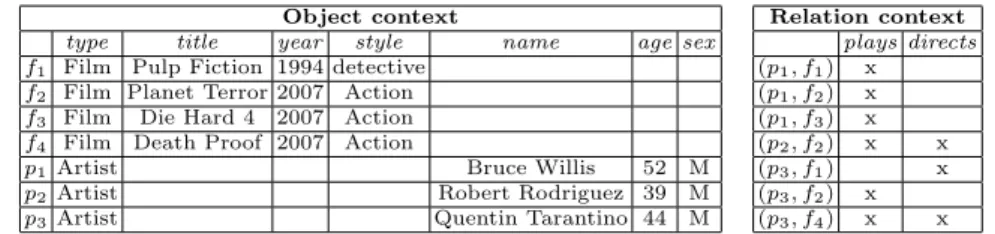
Example 1 (The film and artist context). Here we consider the context of Fi-gure 1 about films and artists. The first row is to be read:

d1(f1) = {title : P ulp F iction , year : 1994 , style : detective} In this example, L1= P(A×LV

1) is a composite logic, where a1:v1∈ A×LV1 is called a valued logical property and represents an attribute followed by its value. A and LV

1 are logics about attributes and values, × enables to define the product of two logics, and P enables to reason on sets of formulas of a logic. A composite logic L includes a composite language L and a composite subsumption relation v. In this example, v1 correponds to a variant of set-theoretic inclusion where subsumption of values of the same attributes are taken into account. When querying, this enables to use patterns over values of properties. For instance, {year : 1994 , style : Detective} v1 {year : >= 1990}. Other examples will be given in Section 4, but for a detailed explanation of the mechanism of logic composition, the reader should refer to [8].

The relation context is a kind of logical context, whose objects are pairs of objects of an object context, and there is an inverse operation for both objects and formulas.

Definition 3 (relation context). Let K1 = (O, L1, d1) be an object context. A relation context is a triple K2= (R, L2, d2), where:

– R is a set of pairs (o1, o2) ∈ O × O. Each pair (o1, o2) represents an ordered binary relation from o1 to o2. Two mappings start and end are defined over R s.t. start((o, o0_{)) =def oand end((o, o}0_{)) =def o}0_{. Furthermore, R is closed} with an inverse operation−1_{, i.e. for every pair r ∈ R, start(r}−1_{) = end(r)} and end(r−1_{) = start(r).}

Object context

type title year style name age sex f1 Film Pulp Fiction 1994 detective

f2 Film Planet Terror 2007 Action

f3 Film Die Hard 4 2007 Action

f4 Film Death Proof 2007 Action

p1Artist Bruce Willis 52 M

p2Artist Robert Rodriguez 39 M

p3Artist Quentin Tarantino 44 M

Relation context plays directs (p1, f1) x (p1, f2) x (p1, f3) x (p2, f2) x x (p3, f1) x (p3, f2) x (p3, f4) x x

Fig. 1.An object context about artists and films, and the corresponding relation

con-text. Relations plays−1_{and directs}−1_{are not explicitly described, but can be}

automat-ically infered from the relation context.

– L2= (L2,v2, .−1_{) is a logic of relations. L2 is a language of formulas used} to described relations. v2 is a subsumption relation, and (.−1_{) denotes an} inverse operation over formulas, considering the inverse of relations s.t. for every f2, g2∈ L2, the following axioms are satisfied:

• (f−1

2 )−1≡2f2 (where f2≡2g2=deff2v2g2∧ g2v2f2), • f2v2g2 ⇔ g−1

2 v2f2−1.

– d2: R → L2is a mapping from pairs of objects to their description expressed as a logical formula. d2 is compatible with the inverse relation, i.e. ∀r ∈ R, d2(r−1_{) ≡2d2(r)}−1_.

The extent of an L2-formula q2 over a relation context is the set of pairs of objects that are related by a relation subsumed by q2.

Definition 4 (relation extent). Let K2 = (R, L2, d2) be a relation context, and q2∈ L2 be a query. The relation extent of the query q2 is defined by

ext2(q2) =def {r ∈ R | d2(r) v2q2}.

Example 2 (The playing and directing relation context). We now consider the relation context of Figure 1 indicating who plays in a film and who directs it. For instance, from this context, we can read:

d2((p3, f1)) = {directs} and d2((f1, p3)) = {directs−1_}

d2((p2, f2)) = {plays, directs} and so d2((f2, p2)) = {plays−1_{, directs}−1_} In this case, L2 = P(Ro) where Ro = {plays, plays−1_{,directs, directs}−1_{} is} a logic of roles. Ro corresponds to the different roles an artist can have in a film, and vice versa. The subsumption relation v2=⊇. (.−1_{) maps a set of roles} to the set of its inverse roles. For instance, {plays, directs} v2 {directs} and {plays}−1_{= {plays}−1_}.

3.2 Querying

In LCA, queries include criteria on both objects and relations. So, for the purpose of querying and navigation, a new context K = (K1, K2), combining the object and relation contexts, is considered. In the same way, a combined query language Lis defined for representing expressive queries.

Definition 5 (combined context and language). Let K1 be an object con-text, and K2 be a relation context. K = (K1, K2) is the combined context, that gathers the individual descriptions of objects and their relationships to each oth-ers. The combined language L is defined as follows:

L→ > | ⊥ | L1| ∃L2.L| ∀L2.L| ¬L | L u L | L t L.

This language is the language of the description logic ALC [9], except atomic concepts are replaced by object formulas (coming from L1), and atomic roles are replaced by relation formulas (coming from L2). The previous definitions of object and relation extents are used as the basis for a combined extent that computes the extent of a combined query. The semantics behind its definition is the same as in description logics, except the closed world assumption is used instead of the open world assumption (e.g., the extent of the negation of a formula is always the complement of the extent of this formula).

Definition 6 (combined extent). Let K = (K1, K2) be a combined context, and q ∈ L be a combined query. The combined extent of q is defined by the recursive set of definitions:

– ext(>) =def O – ext(¬q) =def O \ ext(q)

– ext(⊥) =def ∅ – ext(q u q0_{) =def ext(q) ∩ ext(q}0₎ – ext(q1) =def ext1(q1), where q1∈ L1 – ext(q t q0_{) =def ext(q) ∪ ext(q}0₎ – ext(∃q2.q) =def{o | ∃r ∈ ext2(q2).(start(r) = o ∧ end (r ) ∈ ext(q))} – ext(∀q2.q) =def{o | ∀r ∈ ext2(q2).(start(r) = o ⇒ end (r ) ∈ ext(q))} The formula ∃q2.q can be understood as having at least one image through relation q2 that satisfies the formula q. Whereas ∀q2.q can be understood as having all images through relation q2 that satisfy q.

Definition 7 (query reversal). The query reversal is a query transformation defined as follows:

rev(q0_{u ∃q2.q}00_,∃q2.q00_{) = q}00_{u ∃q}−1

2 .q0 with q0, q00∈ L, q2∈ L2.

Query reversal allows to traverse backward relations already mentioned in a query. This allows to change the point of view by considering either one side of a relation or the other. This is useful because the query ∃q−1

2 (∃q2.q0) is not always equivalent to the query q0_.

3.3 Navigating

As seen before, query reversal already enables to navigate between queries. More-over, in order to help users in building queries, a subset of navigation links can be computed for any query in order to refine it. These navigation links are taken in a finite vocabulary, whose elements are called features. We assume that the set of features for an object context K1 (resp. relation context K2) is given by a user-defined function, called f eat1(K1) (resp. f eat2(K2)). In most cases,

f eat1(K1) (resp. f eat2(K2)) contains at least the subset of L1 (resp. L2) that is used to describe objects, and the subset of patterns of L1 (resp. L2) that users have already entered in queries. Those two vocabularies need to be combined in order to provide a navigation vocabulary over a combined context. It has been proved [3] that the subset of the combined language useful to build navigation links can be restricted to:

Definition 8 (combined vocabulary). Let K = (K1, K2) be a combined con-text. The combined vocabulary is recursively defined as the set of features

feat(K) =def feat1(K1) ∪ {∃x2.x| x2∈ feat2(K2), x ∈ feat(K)}. Features coming from K1are called object features, whereas those coming from K2 are called relation features. As a query ∀q2.q can be rewritten as ¬∃q2.¬q, there is no need for ∀ quantifier in relation features. Given a current query q ∈ L, only features occuring in the extent of q are presented to users as further query increments.

Definition 9 (query increments). Let K = (K1, K2) be a combined context, and a query q ∈ L. A feature x ∈ feat(K) is a query increment if it has a common instance with the query q, i.e. ext(q) ∩ ext(x) 6= ∅.

Object features and relation features can both be used as query refinements, but relation features can also serve as paths to go through. A relation feature ∃q2.q0_{and may be used go from a query q to q u ∃q2.q}0_{(refinement) or q}0_{u ∃q}−1

2 .q (relation traversal). In order to facilitate the browsing of query increments, these navigation links are partially ordered according to subsumption. This requires to define subsumption between features by combining object and relation sub-sumptions.

Definition 10 (combined subsumption). Let K = (K1, K2) be a combined context. The combined subsumption v between features in feat(K) is defined by

xv y =def    xv1y if x, y ∈ L1 x2v2y2∧ x0 _{v y}0 _{if x = ∃x2.x}0_{, y= ∃y2.y}0 _{(f or some x}0_{, y}0 _{∈ L)} f alse otherwise

Example 3 (Query refinement, relation traversal and query reversal). We con-sider the film and artist context, and using the different ways of navigation, we progressively build a query. We start from the most general query qt0= >.

1. We start by refining qt0with the object feature Style:Action to select action films: qt1= > u style:Action = style:Action.

2. Then, we use the relation feature ∃plays−1_{.(name:”Quentin Tarantino”) to} refine the query: qt2= style:Action u ∃plays−1_{.(name:”Quentin Tarantino”).} 3. We choose then to traverse the relation directs−1 _{using the relation feature} ∃directs−1_{.(>). Now qt3 = > u ∃directs}−1_{.(qt2) denotes the artists who} direct an action film in which Quentin Tarantino plays.

4. We are then able to restrict to artists that are men: qt4= qt3u sex:M . 5. Last, we decide to come back to the selected films using the query reversal

on relation direct−1 _{traversed in qt3. The new query qt5 is equal to:} style:Action u plays−1_{.(name:”Quentin Tarantino”) u ∃directs}−1_{.(sex:M ).}

4

LCA applied to the Geographical Domain

In the sequel, we first present a logic Lg1over geometries that enables to describe and reason about the spatial properties of geographical objects. Then, we give two examples of spatial relations defined as logical relations using LCA: a Eu-clidean distance relation defined as L[m]2 and a set of topological relations defined as LT opo₂ . Especially, we describe the logical reasoning over these kinds of spatial relations.

4.1 Spatial Properties

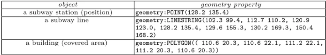
As introduced in Section 3, the object context contains the description of objects expressed as a conjunction of logical properties. To describe the spatial charac-teristics of a geographical object, we use a particular logical property, called the geometry property. The geometry property is a valued property whose name is geometryand whose value represents the shape of the geographical object. This value corresponds to a textual description of the geometry, expressed in the Well Known Text (WKT) format [10] defined by the Open Geospatial Consortium. Like most other geographical data formats, WKT encompasses the location in the shape description. In fact, the shape is defined as a sequence of absolute coordinates determining the spatial border of the geographical object. Examples of geometry properties are presented in Table 1. The domain of values of the ge-ometry property is defined by a specialized logic over geometries: Lg1= (L

g 1,v

g 1).

object geometry property a subway station (position) geometry:POINT(128.2 135.4)

a subway line geometry:LINESTRING(102.3 99.4, 112.7 110.2, 120.9 123.0, 128.2 135.4, 129.6 155.3, 130.2 169.3, 150.4 168.2)

a building (covered area) geometry:POLYGON(( 110.6 20.3, 110.6 22.1, 111.2 22.1, 111.2 20.3, 110.6 20.3))

Table 1.Three simple spatial descriptions illustrating point-wise, linear and area

re-presentation of geographical objects.

Lg₁ is equal to the WKT language, and vg1 corresponds to the inclusion of geometries. According to Lg1, the value g =POLYGON((110.6 ... 20.3)) repre-sents all geometries that are entirely inside g. For instance,

POINT(0.0 0.0)vg

1 POLYGON((-1.0 -1.0,-1.0 1.0,1.0 1.0,1.0 -1.0,-1.0 -1.0)).

When querying for geographical objects, a user has thus the ability to draw an area of interest on a map, and Lg₁ can be used to retrieve all objects located in-side the polygon corresponding to the drawn area. A more detailed explanation of the use of Lg₁ can be found in [1].

4.2 Spatial Relations

Spatial relations are implicitly derived from to the geographical description of objects. The distance relation and the topological relations are function of the location and the shape of objects.

Distance Relation Our first example of a spatial relation is the distance be-tween objects. In the following, we consider only the case where coordinates of geographical objects are expressed in the same projected coordinate system, which corresponds to the common practice in GIS. We define the distance dist between two points as the Euclidean distance. The distance distg between two geometries g1 and g2 corresponds to the minimun distance between a point of g1 and a point of g2:

∀g1, g2, distg(g1, g2) = min{dist(p1, p2) | p1∈ g1, p2∈ g2}

With LCA, distg can be represented with a logic of relations L[m]2 . Formulas take the form of valued attributes. The attribute name is distance and its values correpond to a distance expressed as a real number in the metric system. Intervals and several metric symbols, e.g. m, cm or km can be used as patterns. As a distance relation is symmetric, f−1

2 = f2 for all f2 ∈ L [m]

2 . We give some examples of formulas from L[m]2 , their inverse and their ordering w.r.t. v

[m] 2 :

distance:100m v[m]₂ distance: (being distant of 100m is being distant)

dist:1km v[m]₂ distance:1000m (1km is the same as 1000m)

distance:1km v[m]₂ distance:in [10m,1km] v[m]₂ distance:>=100m

(distance:1km)−1_≡[m]

2 distance:1km

The logic L[m]2 enables queries in the form ∃(distance:<=d) . f1, which selects all objects within a distance less or equal to d of objects described by f1. This kind of queries corresponds to a fundamental functionality of GIS. This is a common way to define a buffered area, i.e. an area determined by both: a set of objects of interest (f1) and a distance relation (distance:<=d). For instance, the following query q1 selects fields close to a river:

q1 = type:field u ∃(distance:<=20m) . type:river

Furthermore, distance formulas can be combined and even nested to build complex queries. For instance consider the query q2 dealing with apartments:

q2 = (apType:T3 t apType:T4) u ∃(distance:<=500m ). type:garden u

∃(distance:<=200m ). (type:busStop u ∃(travel time:<=10min ).

(type:busStop u ∃(distance:<=200m ). place:’IRISA’))

Query q2selects 3- or 4-rooms apartments that are close (less than 500m) to a public garden, and that are near (less than 200m) a bus stop from where it takes less than 10min by bus to reach another bus stop that is close to IRISA (less than 20m).

Topological Relations Topological relations are binary relations describing the spatial position of an object w.r.t another object. These relations are quali-tative, they give information about the spatial organisation of objects indepen-dently from their size, shape or distance. The expression of topological relations is a domain that has already been widely investigated [7]. Several classifications have been proposed, some of which based on Galois lattices [11]. In the follow-ing, we consider a taxonomy of topological relations over regions [12], including the 8 base relations of the RCC8 model [13] and 7 intermediate relations (see Figure 2). Each organisation of 2 polygonal geometries in a 2-dimension space can be expressed as one of the 8 base relations. For the purpose of information retrieval, this classification has the advantage of being quite simple with only few relations (15) and understandable intermediate relations.

A B Disjoint

A B A B

Inside Contains Overlapping T

A B A B

A B B B A

Inside_s Inside_t Equal Contains_sContains_t Overlapping_s Touching Connected

Fig. 2.A taxonomy of spatial relations over 2 regions proposed in [12]. Leafs of the

taxonomy correspond to the 8 base relations of the RCC-8 model.

With LCA, we consider a logic of relations LT opo2 to handle these topological relations. Formulas of LT opo2 are the 15 spatial relations, and the ordering of vT opo₂ follows the taxonomy of Figure 2. For instance, equal vT opo2 connected. The > stands for the general relation being spatially related, which we consider always true between two geographical objects. Notice also the symmetric prop-erties between relations: inside−1 _{= contains, inside t}−1 _{= contains t,} inside s−1_{= contains s, and r}−1_{= r for all other relations. We now suppose} that for each couple of area objects (o1, o2) of the object context, the 2 RCC-8 relations describing the position of o1w.r.t. o2, and reciprocally, have been added in the relation context. At the moment, the computation of the relevant relation is done by an external GIS module. The logic LT opo2 allows to build queries such as:

q1 = type:building u ¬ ∃touching . (type:building)

q2 = type:cityBlock u ∀contains . (type:lodging)

q3 = type:road u ∃touching .(place:’my home’) u

∃connected .(type:garden u ∃contains . (type:lake))

The query q1selects all non-terraced houses, q2, residential areas, and q3, roads next to my home and leading to a public garden having a lake.

5

Navigation based on Spatial Relations

One asset of LCA is to combine querying and navigation in order to make infor-mation retrieval easier and faster. From any query, navigation is enabled through a set of navigation links that update the query, and eventually through query reversal. To facilitate the navigation, query increments are ordered in a navi-gation tree, according to the subsumption relation (v). In previous works [1], we have already introduced a graphical interface that enables navigation inside geographical data, however it was not dealing with relational properties. This interface is composed of a query box, a map area, and a navigation tree. The query box recalls the current query, i.e. the navigation context and is manually editable by the user. By analogy with file systems, the current query is called the working query (wq). The map area is a cartographic representation of the explored context and enables to graphically select regions of interest as graphical query increments. The navigation tree is a visual representation of the partially ordered set of query increments, which are computed on demand and always rel-evant w.r.t. wq. In the following, we present a navigation tree allowing relational navigation through spatial relations. The query box has also been enhanced with the query reversal transformation. Non nested relation features appearing in wq are in fact hyperlinks that enable to traverse backward those relations.

To illustrate the use of navigation, we consider the following situation, where a traveller arrives in an unknown (fictive) city and looks for information about several points of interest, including lodging, lunch, recreation or transport offers. To help himself, he relies on a LIS device that let him query and navigate the city map context using a navigation tree and a query box. The set of objects O of the context corresponds to the points of interest, the streets and the po-sition of our traveller. The individual spatial and non-spatial properties of the objects are described with a logic Lcity1 = P(A × (LV1 ∪ L

g

1)). The distance re-lations and the topological rere-lations the objects share are expressed with the logic Lcity2 = P(L

[m] 2 ∪ L

T opo

2 ), allowing that descriptions of relations can include formulas from either L[m]2 or L

T opo

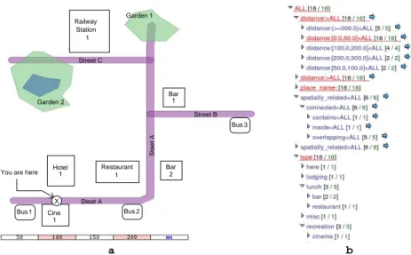
2 . The description of the city map is presented in Figure 3a. Topological relations between all pairs of objects have been com-puted beforehand using a GIS. The disjoint relations, not relevant for this case of navigation, have not been expressed. However, objects disjoint from others can be accessed through the ¬∃connected .> increment. Distance relations have also been computed beforehand between each point of interest and its neighbour streets. For instance, the “Bus stop 1” touches the “Street A”, and the “Bar 2“ is within a distance of 10 meters of “Street A”.

5.1 The Navigation Tree

The navigation tree related to the citymap context is presented in Figure 3b. It displays information about the type of geographical objects (type), their name (place name), and about the spatial relations they share (distance and spatially related for topological relations). Query increments, also called

a Bar Bar Cine Bus Bus Bus Railway Station X 1 1 1 Garden 1 Garden 2 Steet A Steet A Street C 2 3 2 1 Street B 1 Restaurant Hotel 1 You are here

b

Fig. 3.Map of a city unfamiliar to our traveller (on the left), and the corresponding

navigation tree (on the right).

features, may be of two kinds (see Section 3.3). Object features are proper-ties shared by at least one object of wq. For instance, in the citymap navi-gation tree, there is one lodging object. Relation features denote a relation between some objects of the current query, with at least one other object of the context. Relation features correspond to ∃x2.xnavigation links, but are ex-pressed in the navigation tree with direction symbols > and <. For instance, in the citymap navigation tree, 6 objects are spatially related to another object. The feature spatially related>ALL corresponds to ∃spatially related.>, and spatially related<ALL corresponds to ∃spatially related−1_{.>. In the tree of} Figure 4, both features distance:>ALL and distance:<ALL are represented, altougth they are redundant because the distance relation is symmetric. This is also true for some topological relations. In the future, a special handling of symmetric relations is planed.

Each node of the tree represents a feature which can be used to change wq. When a node is expanded, this entails dynamically the computation of features that are specializations of the feature of this node. Then, the new features appear as its children in the tree. For instance, in Figure 3b, the taxonomy of points of interest is visible under the feature type, and distance intervals are visible under the distance:<ALL feature. The root of the tree is ALL, i.e., the most general formula. Each node of the tree is rendered with an icon, a label, two numbers, and possibly an arrow. The label is the formula representing the feature. The style of the label is informative: underlined labels correspond to formulas shared by all the objects in wq, whereas blue labels indicate properties that discriminate them. The two numbers indicate a proportion: the count of objects in wq that the feature leads to, i.e. the support, out of the count total of objects sharing the feature. In Figure 3b, the counts next to the feature distance:[0.0,50.0]<ALL are both equal to 16, i.e. all geographical objects of the citymap context are

within 50 meters of another object. Three actions are possible in the tree: (1) displaying more (resp. less) navigation links, i.e. expanding (resp. collapsing) a node by acting on its icon; (2) refining wq by selecting a label; (3) traversing a relation by selecting the arrow next to the node.

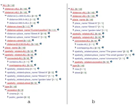
5.2 Example of Navigation

Just suppose that our traveller has left his luggage at the hotel and wants to have some recreation before having lunch. He looks at his LIS device, provides it with a new geographical object corresponding to its position (which we denote here). This entails the addition of distance relations (already displayed in the tree of Figure 3b) between the object here and the other points of interest of the context; the distances are computed on the basis of the shortest path, following streets. He then queries the system with:

wq= recreation

The LIS system provides him with the updated navigation tree of Figure 4a. The taxonomy of geographical objects (under feature type) has been reduced and now only contains the recreation feature. By expanding this feature, he can see 2 sub-features indicating 2 types of available recreation: cinema and public garden. The first count of the feature recreation indicates that only 3 geographical objects correspond to recreational areas. The other features of the tree have also been updated. For instance, we can see that 2 recreation places are connected to “Street A”.

Prefering being outside, our traveller decides to restrict his choice to public gardens not too close to his actual position. So, in the tree, he selects the feature public garden, and manually modify wq so as to select public gardens located at more than 350 meters:

wq= public garden u ∃(distance :>= 350.0m).here

The navigation tree has been updated anew, and indicates him that two public gardens satisfy the query. By looking at the navigation tree, he can see the query increment connected>ALL denoting that some information about the topologi-cal organization of these gardens is available. Wanting more details about the environnement of the gardens, he traverses the connected relation by selecting the arrow next to the feature. This updates wq to:

wq= ∃connected−1_{.(public garden u ∃(distance :>= 350.0m).here)}

The navigation tree now displays information concerning 3 geographical objects topologically linked with a public garden (see Figure 4b). By looking at the feature type, he can see that two of these objects are streets leading to a garden, and that the other one belongs to the miscellaneous category. Just by selecting the misc feature and looking at the feature place name, our traveller can see that it corresponds to a lake which is in fact inside a public garden. To retrieve the corresponding garden, he then just has to follow backward the connected relation (query reversal) by clicking on connected−1 _{in the query box. Then wq} becomes:

a

b

Fig. 4.The citymap navigation tree at two different steps. In tree a, wq = recreation,

in tree b, wq = ∃connected−1_{.(public garden u ∃(distance:>=350.0m).here)}

6

Benefits of using LCA to Query Geographical Data

Regarding data organisation and retrieval, GIS have been widely influenced by Relational Database Management Systems (RDBMS) [14]. Most of the time, geographical information is structured into thematic layers, i.e., a layer for the streets, another for the points of interest, etc. Recently, XML-based formats for geographical data [15] allow to consider collections of heterogeneous geographical objects. But in every instance, retrieving data is done using querying interfaces and querying languages (XQuery-like or SQL-like) that integrate spatial predi-cates.

Our proposal of using LCA to manage geographical data not only enables to build queries similar to traditional GIS queries, it also offers a flexible organi-zation of the data. Our data model is centered on the geographical object and enables to consider each collection of objects that share a common description expressed by a query q as a kind of flexible layer that can serve as a basis for fur-ther processing. In GIS, traditionally, querying for data disseminated into several collections implies making as many sub-queries as collections and merging the results. This service is automatically provided by LCA but requires the descrip-tions of similar objects to be comparable. Concerning the querying capabilities, firstly, the querying language available in LCA (see Section 4), combined with the spatial logics of distance relation and topological relations, already enables to express most of the queries traditionally used in a GIS, as shown in Section 4.2.

For instance, concerning spatial queries, the formula ∃(distance:<=d).q0_enables to consider buffered areas of radius d around geographical objects described by q0_{. Moreover, like with GIS traditional languages, these buffered areas can be} combined using Boolean operators and nested in other spatial predicates. Sec-ondly, the expressivity of LCA relies for one part on the sub-logics used to reason on object descriptions. But once a new logic has been designed for a particular purpose, e.g. comparing areas derived from geometrical descriptions, it can be added to the system without reconsidering the whole theory. This makes the LCA querying language powerful as it can be easily extended, and customized to handle particular data. Currently, compared to SQL or XQuery, LCA lacks the ability to express agregates, although this is an interesting field we plan to investigate.

An advantage of LCA compared to traditional GIS is the navigation tree. Even in dedicated map search tools such as the proximity business search of Google Maps , the results are always delivered as a flat textual list with bullets on a map, where no indication is given on the structure of the answer and on how to refine it. In comparison, the navigation tree offers at least three assets. First, the navigation links give at a glance a summarized description of the currently selected dataset. Then, these navigation links provide a querying vocabulary which allows to build a query from scratch even with no knowledge about the data. Last but not least, the navigation links enable to refine the current query in a relevant way, i.e., ensuring the answer will be reduced but not empty. Giving aid in the building of queries is also a contribition of the VISCO system [12]. In VISCO, description logics are used to query a spatial database in a visual way. Like our prototype, VISCO enables to represent and to reason about spatial properties, e.g. area or perimeter, and topoligical relations of geographical objects. In addition to querying capabities, VISCO also assists the user with query completion based on terminological default reasoning. However, contrary to our proposal, augmented queries may lead to empty answers because it does not take into account the content, but only the logic.

LCA also brings a new kind of navigation, the relational navigation. Con-sidering a set of objects O that are instances of a query q and in relation r with other objects O0 _{described by f , i.e. the link ∃r.f is visible in the tree, one} can directly jump to the related objects O0_{. In the geographical domain, this} provides facilities when querying data organized in several thematic collections. Compared to traditional GIS practices, this kind of navigation prevents the user from building sub-queries corresponding to search criteria depending on several layers and then combining or nesting these sub-queries in the right way. With the relational navigation, the search process can be fully incremental, and does not impose any order on the building of a query.

7

Conclusion

In this paper, we first show that LCA is a framework that enables to easily model spatial relations between geographical objects. Valued spatial relations such as

distance can be expressed in an intuitive manner thanks to the expressivity of logics. Furthermore, thanks to the partial ordering between logical relations, LCA naturally integrates taxonomies of relations, such as topological relations. Then, we present an original way to explore geographical data, using a navigation based on spatial and non-spatial properties of objects, as well as on the spatial relations between geographical objects. Especially, we illustrate the benefits of this paradigm of geographical data exploration provided by LCA, compared to traditonal GIS querying capabilities.

In the future, we plan to make the update of relations automatic and incre-mental when the description of geographical objects changes, e.g. their position. We also plan to work on a graphical representation of relation features in order to enhance the readibility of the navigation tree and to assist the user in the building of queries involving spatial relations.

References

1. Bedel, O., Ferr´e, S., Ridoux, O., Quesseveur, E.: Exploring a geographical dataset with GEOLIS. In: DEXA Workshop ACKE’07. (2007)

2. Ferr´e, S., Ridoux, O.: An introduction to logical information systems. Information Processing & Management (2004)

3. Ferr´e, S., Ridoux, O., Sigonneau, B.: Arbitrary relations in formal concept analysis and logical information systems. In: ICCS. LNCS 3596, Springer (2005) 166–180 4. Wille, R.: Conceptual graphs and formal concept analysis. In: ICCS ’97, London,

UK, Springer-Verlag (1997) 290–303

5. Rouane, M.H., Huchard, M., Napoli, A., Valtchev, P.: A proposal for combin-ing formal concept analysis and description logics for mincombin-ing relational data. In Kuznetsov, S.O., Schmidt, S., eds.: ICFCA. LNCS 4390, Springer (2007) 51–65 6. Michael J. de Smith, M.F.G., Longley, P.A.: Geospatial Analysis: A Comprehensive

Guide to Principles, Techniques and Software Tools. Troubador Publishing (2007) 7. Cohn, A.G.: Qualitative spatial representation and reasoning techniques. In: KI ’97: Proceedings of the 21st German Conference on Artificial Intelligence. (1997) 8. Ferr´e, S., Ridoux, O.: Logic functors: A toolbox of components for building

cus-tomized and embeddable logics. Research Report RR-5871, Irisa (March 2006) 9. Donini, F.M., Lenzerini, M., Nardi, D., Nutt, W.: The complexity of concept

languages. Information and Computation 134 (1997) 1–58

10. Herring, J.R.: OpenGIS Implementation Specification for Geographic information (06-103r3). Open Geospatial Consortium (OGC). (2006)

11. Napoli, A., Ber, F.L.: The galois lattice as a hierarchical structure for topological relations. Ann. Math. Artif. Intell. 49(1-4) (2007) 171–190

12. Wessel, M., Haarslev, V., M¨oller, R.: Visual spatial query languages: A semantics

using description logic. In: Diagrammatic Representation and Reasoning. Springer (2000)

13. Randell, D.A., Cui, Z., Cohn, A.: A Spatial Logic Based on Regions and Connec-tion. In Nebel, B., Rich, C., Swartout, W., eds.: KR’92. Morgan Kaufmann, San Mateo, California (1992) 165–176

14. Laurini, R., Thompson, D.: Fundamentals of Spatial Information Systems. Aca-demic Press Limited (1992)

15. Cox, S., Daisey, P., Lake, R., Portele, C., Whiteside, A.: Geography Markup Language (GML) Encoding Spec. Open Geospatial Consortium (OGC). (2004)