Range error analysis of an integrated time-of-flight, triangulation, and photogrammetric 3D laser scanning system

Publisher’s version / Version de l'éditeur:

Vous avez des questions? Nous pouvons vous aider. Pour communiquer directement avec un auteur, consultez la première page de la revue dans laquelle son article a été publié afin de trouver ses coordonnées. Si vous n’arrivez pas à les repérer, communiquez avec nous à PublicationsArchive-ArchivesPublications@nrc-cnrc.gc.ca.

Questions? Contact the NRC Publications Archive team at

PublicationsArchive-ArchivesPublications@nrc-cnrc.gc.ca. If you wish to email the authors directly, please see the first page of the publication for their contact information.

https://publications-cnrc.canada.ca/fra/droits

L’accès à ce site Web et l’utilisation de son contenu sont assujettis aux conditions présentées dans le site

LISEZ CES CONDITIONS ATTENTIVEMENT AVANT D’UTILISER CE SITE WEB.

SPIE Proceedings, 2000

READ THESE TERMS AND CONDITIONS CAREFULLY BEFORE USING THIS WEBSITE. https://nrc-publications.canada.ca/eng/copyright

NRC Publications Archive Record / Notice des Archives des publications du CNRC :

https://nrc-publications.canada.ca/eng/view/object/?id=3803dbf7-faa3-45f9-8926-14418bab1f2f

https://publications-cnrc.canada.ca/fra/voir/objet/?id=3803dbf7-faa3-45f9-8926-14418bab1f2f

NRC Publications Archive

Archives des publications du CNRC

This publication could be one of several versions: author’s original, accepted manuscript or the publisher’s version. / La version de cette publication peut être l’une des suivantes : la version prépublication de l’auteur, la version acceptée du manuscrit ou la version de l’éditeur.

Access and use of this website and the material on it are subject to the Terms and Conditions set forth at

Range error analysis of an integrated time-of-flight, triangulation, and

photogrammetric 3D laser scanning system

National Research Council Canada Institute for Information Technology Conseil national de recherches Canada Institut de Technologie de l’information

Range Error Analysis of an Integrated Time-of-Flight,

Triangulation, and Photogrammetry 3D Laser

Scanning System*

F. Blais, J.-A. Beraldin, and S.F. El-Hakim

April 2000

Copyright 2001 by

National Research Council of Canada

Permission is granted to quote short excerpts and to reproduce figures and tables from this report, provided that the source of such material is fully acknowledged.

*

In Laser Radar Technology and Applications V, Proceedings of SPIE’s Aerosense 2000 Vol. 4035, 24-28 April 2000, Orlando, FL.

Range Error Analysis of an Integrated Time-of-Flight, Triangulation,

and Photogrammetric 3D Laser Scanning System

F. Blais, J.-A.Beraldin, S. El- Hakim

National Research Council of Canada

Institute for Information Technology

Ottawa, Ontario, Canada

ABSTRACT

A 3-D laser tracking scanner system analysis focusing on immunity to ambient sunlight and geometrical resolution and accuracy is presented in the context of a space application. The main goal of this development is to provide a robust sensor to assist in the assembly of the Space Station. This 3-D laser scanner system can be used in imagery or in tracking modes, using either time-of-flight (TOF) or triangulation methods for range acquisition. It uses two high-speed galvanometers and a collimated laser beam to address individual targets on an object. In the tracking mode of operation, we will compare the pose estimation and accuracy of the laser scanner using the different methods: triangulation, TOF (resolved targets), and photogrammetry (spatial resection), and show the advantages of combining these different modes of operation to increase the overall performances of the laser system.

Keywords: Laser scanner, 3D, ranging, tracking, light immunity, photogrammetry, spatial resection, triangulation,

time-of-flight.

1. INTRODUCTION

Electro-optical imaging system analysis provides an optimum design process through appropriate tradeoff analyses [1]. A comprehensive model will include the target, background, the properties of the surrounding environment if applicable (e.g. atmosphere), the optical system, detector, electronics, and human interpretation of the data. While any of these components can be studied in detail separately, the electro-optical system cannot. Only complete end-to-end analysis (scene-to-observer) permits system optimization. Finding the optimum design is an iterative decision process. Each step in the design process requires a tradeoff analysis and many performance parameters can only be increased at the expense of another [2].

Key to the design of an electro-optical system is the overall application. Although there is a desire for a single electro-optical imaging system to perform all functions, this is still far from being possible even though new technological developments are narrowing the gap. As the system complexity increases and technology advances, it is increasingly necessary to define performance requirements for each subsystem to insure that the overall system requirements are met. This is an ever-increasing challenge to the system analyst.

The Canadian contribution to the International Space Station is the Mobile Servicing System, which will support the assembly, maintenance, and servicing of the space station. A fundamental component of the Mobile Servicing System for the automation of space-related activities is the vision system, which will play a major role in both space station assembly and space station maintenance operations.

Unfortunately, the presence of the sun or any other strong sources of light adversely affect the quality of the conventional methods that rely on standard video images, e.g. closed circuit camera on-board shuttle. Poor contrast between features on the object and background makes these conventional video images difficult to analyze. Figure 1 shows a typical example of

*

video images obtained on orbit that illustrate potential problems a vision system will encounter during normal operation. Camera saturation, insufficient light and shadows are very serious problems that limit the normal operation of conventional video-based vision systems.

A more subtle case for automated machine vision system is concerned with lighting gradients (cast shadows) as illustrated in Figure 1b, which requires both extended dynamic range for the video camera and sophisticated image processing algorithms. Although this seems a-priori a straightforward problem for the human eye (brain), it is not as simple for limited dynamic range vision systems. It is therefore very important that any complementary systems like a laser scanner be robust to operational conditions such as sun interference, saturation, shadows, or simply insufficient light.

Figure 1: Examples of the effect of sun illumination and earth albedo on video image cameras: a) saturation, and b) shadow

effects. The Space Vision System [3,4] uses the known location of the B/W targets to compute the pose of the object(s).

Table 1: Conditions for ambient illumination and their effect on the Laser Scanner System.

Illumination conditions

Possible effect on laser scanner

Normal conditions None – normal conditions

Partial target shadowing None – outside instantaneous field of view of camera Full target shadowing Reduced accuracy – Distortion on signal or saturation Saturation (Field of view) Minimal – normally outside instantaneous FOV of camera No Light (Dark) None - Ideal for laser scanner

Estimated percentage of "conditions" of operation in orbit

60% Normal conditions 35% Shadow conditions <5% Saturation & poor illumination <1% Back illumination

The laser-based range scanner approach presented here offers the advantage of being close to 100% operational throughout the changing illumination conditions in orbit. The technique combines time-of-flight and triangulation ranging methods, and is designed to be insensitive to background illumination such as the earth albedo, the sun, and most of its reflections. The laser scanner uses two principal modes of operation:

• Imaging produces a dense raster type 3D (range) image of the object.

• Real-time tracking of multiple targets on object(s): compute the orientation and position of the object in 3D space.

One of the unique features of this laser scanner is its potential to combine in a single unit different ranging and object pose estimation methods:

• Triangulation-based method for short to medium distance measurements (<5-10 m)

• Time-of-flight (LIDAR) method for longer range

• Photogrammetry-based technique (spatial resection) and target tracking, compatible with current Space Vision System (SVS) used by NASA.

Using the imaging mode, the main applications include inspection and maintenance; where as, assembly, docking, and any tele-manipulation operations are solved using the tracking mode. Figure 2a shows a 3-D raster image obtained using the laser scanner in raster imagery mode using triangulation. Figure 2b shows a range image acquired using a Time-of-flight method.

a) b)

Figure 2: Raster images acquired using the NRC’s laser scanner, (a) triangulation mode (the range derivative is encoded in grey

levels to amplify the details and the fine structure of the surfaces of the object), and (b) Time-of-Flight mode. In (range information is directly encoded in grey levels).

In tracking mode, the variable resolution laser scanner of Figure 3 tracks in real time targets and/or geometrical features of an object as shown in Figures 4 and 5. The scanner uses two high-speed galvanometers and a collimated eye-safe laser beam at a wavelength of 1.5 µm to address individual targets on the object. Very high resolution and excellent tracking accuracy are obtained using Lissajous scanning patterns [5,6].

Raster Mode

(3-D Image Size) Maximum Refresh Rate(sec) 128 × 128 0.8

256 × 256 3.3 512 ×512 13.1

Tracking mode Maximum Tracking Speed

Single target 6.6 msec Multiple targets 10 msec × Targets

Table 2: Typical acquisition time for the 3-D Laser Scanner

System used in raster and tracking modes; acquisition speed

is 20000 Voxels/sec. Figure 3: Prototype of the 3-D Laser Scanner System. The small targets visible in Figure 1 (small black dots) are currently being used by the Space Vision System [3,4]. Because the exact locations of these features on the object are known, object position is computed from their relative positions in the video images using photogrammetry-based technique known as spatial resection. Obviously tracking compatibility with

these B/W targets is a key aspect for the laser scanner and system sensitivity becomes mostly a question of minimum laser signal power relative to the background light rather than the minimum signal detected and detector electrical noise. Lissajous tracking will be discussed more in detail in section 3.

Figure 4: Principle of tracking using the Lissajous pattern

and a circular target.

Figure 5: Real-time tracking of targets on the simulated

Node and Z1 modules used during the experimentation. Two types of target are visible, Inconel B/W and retro-reflective targets. The system tracks each target sequentially. In this example, one of the targets is in “search mode” (larger Lissajous pattern).

For the Laser Scanner, to operate properly under such severe ambient illumination in orbit, two main aspects must be verified:

• Saturation of the CCD signal

• Signal to Noise Ratio (SNR) between target returned signal and Sun interference

In this paper, the laser scanner signal-to-background noise (SNR) and tracking resolution/accuracy models are presented. Range accuracy using both time-of-flight (TOF) and triangulation methods are compared. In the tracking mode or operation, we will also compare the pose estimation and accuracy of the laser scanner operated in the photogrammetric mode and show the advantages of combining these different modes of operation to increase the overall dynamic accuracy of the laser system. Emphasis is placed on the tracking mode of operation of the laser scanner, usually more stringent than standard imaging because of automation aspects and increased accuracy requirements.

2. LASER SCANNER MODEL

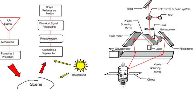
Models must be able to relate design parameters, laboratory measurable, and operational performance. Figure 6 illustrates the major subsystems of an active electro-optical system: projector sources and collimating optics, deflection mechanism, collecting optics, detector, signal conditioning and processing, and final output. The collecting optics images the radiation onto the detector. In the example of Figure 7, the scanner optically moves the detector’s instantaneous field-of-view (IFOV) across the total field-of-view (FOV) to produce an output voltage (signal) proportional to the local scene intensity (produced by ambient light conditions) and the laser light reflected back from a reflective surface.

The detector is at the heart of the electro-optical system because it converts the scene radiation (reflected flux) into a measurable electrical signal. Amplification and signal processing creates a signal in which voltage differences represent scene intensity differences due to various objects in the field-of-view.

The majority of electro-optical quality discussions are centered on resolution and sensitivity evaluation. System sensitivity deals with the smallest signal that can be detected. It is usually taken as the signal that produces a signal-to-noise ratio of

Center of target Tracking Error Target Lissajous Scan Search

unity at the system output. Sensitivity is dependent upon the light-gathering properties of the optical system, the responsivity of the detector, the noise of the system and, for this application, the background flux. It is independent of resolution.

In the case of metrology, resolution is not sufficient and stability and accuracy must also be considered. Resolution has been in use so long that it is thought to be something fundamental, which uniquely determines system performances and is often confused with accuracy. It is often specified by a variety of sometimes-unrelated metrics such as the Airy disk angular size, the detector subtense, or the sampling frequency. Resolution does not usually include the effect of system noise.

Figure 6: Generic sensor operation applied to active

electro-optical systems.

Figure 7: Schematic representation of the auto-synchronized

geometry.

2.1. The Auto-Synchronized Laser Scanner

Figure 3 shows a photograph of the prototype of the auto-synchronized laser scanner developed for this demonstration. The scanner uses a variation of the auto-synchronized triangulation range sensor based on one galvanometer [8]. The system comprises two orthogonally mounted scanning mirrors and a linear discrete-response photosensitive position device (e.g. linear CCD) used for short to medium range measurement (triangulation) [12]. An optional avalanche photo-diode-based Time-of-Flight (LIDAR) ranging module is used for longer-range measurement [7]. Only resolved targets using TOF are considered for this application. Laser illumination is provided using a laser source coupled to a single-mode fiber, either pulsed (TOF mode) or CW (triangulation mode). The laser scanner operates at a relatively eye safe wavelength of 1.5 µm (compared to visible laser wavelengths).

The basic concept of auto-synchronization is that the projection of the light spot is synchronized with its detection as illustrated in Figure 7. The instantaneous field of view (IFOV) of the position sensor follows the spot as it scans the scene. Therefore, an external optical perturbation can potentially interfere with the detection only when it intersects the instantaneous field of view (IFOV) of the scanner. At this level, electronic signal processing is used to filter these false readings to obtain correct 3-D measurement [6]. With synchronization, the total field of view (FOV) of the scanner is related to the scanning angles of the galvanometers and mirrors as opposed to a conventional camera-based triangulation. Here the field of view and image resolution are intimately linked [8]; a large field of view produces a lower pixel resolution. In summary, the instantaneous field-of-view of the scanner plays a major role in the system sensitivity analysis.

2.2. Range measurement

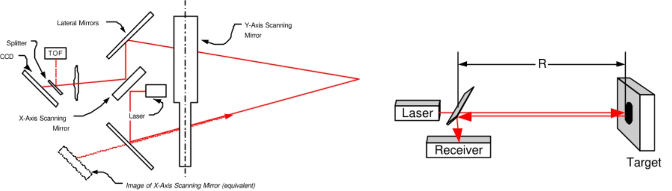
Figure 7 shows the optical geometry of the auto-synchronized laser scanner. The laser scanner system can measure range information for each voxel (3-D pixel) in the scene using two modes of operation: (1) triangulation as illustrated in Figure 8, and (2) time-of-flight shown in Figure 9. It is beyond the scope of this paper to discuss the details of operation of the scanner

Light Source Modulation Focusing & Projection Scene Background Electrical Signal Processing Photodetection Shape Reflectance Motion Collection & Reprojection Y-axis Scanning Mirror CCD TOF Lens Fixed mirror Fixed mirror X-axis Scanning Mirror Galvanometer Galvanometer Object Laser

and the exact mathematical model. This information is available from previous publications where the scanner is operated in imaging mode [8,9,12]. Here, we will use the simplified models illustrated in Figure 10 to model range measurement and to associate object pose estimation obtained using video camera models shown in Figures 11 and techniques discussed in section 4.

Figure 8: Simplified geometry of the laser scanner for the

triangulation mode.

Figure 9: Schematic of the time-of-flight principle.

Figure 10: Simplified geometrical model of the laser scanner

showing the effect of astigmatism between the X and Y scanning axis.

Figure 11: Simplified geometrical model of a simple camera

lens system used by conventional camera and photogrammetric methods.

From [8], knowing that R=z/cos(θ), and from Figure 10, range R can be calculated either using triangulation methods or TOF. The simplified aberrations free model is presented here. For triangulation, range is given by

(1)

where f is the focal length of the lens, d is the triangulation base, θ is the deflection angle following the x-axis, and p is the position of the imaged laser spot of the position sensor (see [8] for details). For the TOF method of Figure 9, range is simply obtained based on the speed of light c and the propagation delay τ of a laser pulse:

(2)

From Figure 10, the x-y-z coordinates of a point are

(3) Rotation X-Axis Rotation Y-Axis X Z Y CCD Lens Dg (0,0,0) φ θ R Y-Axis Scanning Mirror Lateral Mirrors X-Axis Scanning Mirror Laser CCD

Image of X-Axis Scanning Mirror (equivalent) TOF Splitter Rotation X-Axis Rotation Y-Axis X Z Y Camera Lens Laser Receiver Target R ) sin( ) cos(θ d θ p d f R_Trian = ⋅ + 2 τ c R_TOF =

(

)

where θ and φ are the deflection angles, and ψ=Dg/R where Dg is the separation between the two scanning axis shown in

Figure 10. Range R is obtained using either RTrian or RTOF depending on the operating mode of the scanner. Because Dg<<R,

error propagation calculations (in triangulation mode) can be approximated by

(4)

(5)

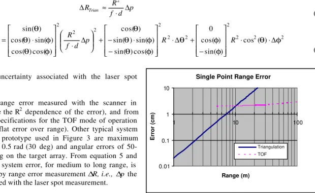
where ∆p is the uncertainty associated with the laser spot measurement.

Figure 12 shows range error measured with the scanner in triangulation (notice the R2 dependence of the error), and from the manufacturer specifications for the TOF mode of operation (notice the almost flat error over range). Other typical system parameters for the prototype used in Figure 3 are maximum deflection angles of 0.5 rad (30 deg) and angular errors of 50-100 µrad, depending on the target array. From equation 5 and Figure 12, the total system error, for medium to long range, is mostly contributed by range error measurement ∆R, i.e., ∆p the

uncertainty associated with the laser spot measurement.

Figure 12: Range error accuracy of the Laser Scanner

System.

3. REAL-TIME TRACKING – LISSAJOUS PATTERNS

Real-time tracking of targets or geometrical features on an object is implemented using Lissajous figures, to obtain good scanning speed and accuracy. Driving the two axis galvanometers with sine waves of different frequency creates a Lissajous pattern [5,6]. The geometrical tracking principle uses both the 3-D range and intensity information on the Lissajous pattern to (a) identify targets on the object or any useful geometrical feature, and (b) to discriminate the target from its background. Lissajous patterns are used to efficiently scan objects at refresh rates exceeding the bandwidth of the mechanical deflection system. The Lissajous tracking pattern is a key feature to increase angular accuracy used during photogrammetric mode of operation of the scanner.

A Lissajous figure is mathematically defined using:

(6)

(7)

where Ax, and Ay are the amplitudes of the Lissajous pattern, Px and Py its position. The Lissajous pattern is defined using the

cycle ratio m:n in the previous equations. The pattern phases are adjusted using ϕx and ϕy.

Figure 4 and 5 illustrate the principle associated with position tracking of a single target using a 3:2 Lissajous pattern (ratio

m:n). Range and intensity data are measured for each of the N points on the scanning pattern. The Lissajous tracking pattern

plays a major role in system resolution (and accuracy).

2 2 2 2 2 2 2 2 2 2 2 ) ( cos ) sin( ) cos( 0 ) cos( ) sin( ) sin( ) sin( ) cos( ) cos( ) cos( ) sin( ) cos( ) sin( φ θ φ φ θ φ θ φ θ θ φ θ φ θ θ ∆ ⋅ ⋅           − + ∆ ⋅           − ⋅ − +       ∆ ⋅           ⋅ =           ∆ ∆ ∆ R R p d f R z y x p d f R RTrian ≈ _⋅ ∆ ∆ 2 x x x P T t m A t x +      ₊ = cos 2π ϕ ) ( y y y P T t n A t y +      ₊ = cos 2π ϕ ) (

Single Point Range Error

0.01 0.1 1 10 1 10 100 Range (m) Error (cm) Triangulation TOF

Different scanning methods and signal processing techniques are used to further increase resolution:

• the natural inertia of the galvanometer-mirror structures that smoothes the scanning pattern and hence increases the pointing accuracy of the tracking system;

• sub-pixel target centroid detection methods to reduce the effects of laser spot resolution on the target;

• pattern position (Px, Py), amplitude (Ax, Ay), and/or phase (ϕx,ϕy) dithering to reduce quantification noise; • pattern direction inversion (-Ax, -Ay), to remove non-constant signal delay and bias;

• data smoothing (e.g. plane/circle fitting).

In practice, the laser scanner angular resolution is limited mostly by two parameters:

• Sub-pixel resolution and size of the target

• Galvanometer mechanical resolution (wobble and jitter) and temperature stability

In Figure 5, the laser scanner scans sequentially different sections of the object. One of the targets is here in the search mode and the scanner uses a larger Lissajous pattern to localize it. When found, the scanner automatically switches from the search mode to the track mode using a smaller Lissajous pattern to increase target centroid accuracy. The laser scanner sequentially scan different sections or targets on one or several objects. The locations of the centroid of the detected targets is fed directly into the existing photo-solution and attitude control modules, based on photogrammetric techniques to compute either the absolute or relative poses (position and orientation) of multiple objects.

4. OBJECT POSE EVALUATION

Object pose evaluation is a complex subject by itself and an in depth mathematical analysis is beyond the scope of this paper. We will rather provide here a qualitative analysis of the method from an empirical point of view. Assuming a set of known coordinates (xo,yo,zo) on a rigid object, the expected location of these targets in the laser scanner 3-D space (x),y),z)) is given

using homogenous coordinates by:

(8)

(9)

(10)

where M is a 4x4 rigid transformation matrix (|M|=1) that maps the object target coordinates in the laser scanner space. The matrix M has 6 unknowns, 3 translations and 3 rotations (yaw-pitch-roll). Object pose estimation consists of evaluating the transformation matrix that will minimize a set of error equations. The most commonly used method minimize the quadratic error between the expected position computed from the previous equation and the laser scanner measurements x-y-z:

(11)

(12)

(13) Different techniques are available to minimize this set of equations such as based on least-squares adjustment, and quaternions. From equation 5 and considering medium to long range applications, the error vector E is highly dependent on the range measurement, R,

(14)

Using the basic lens model of Figure 14 and equation 3, and photogrammetry methods, the collinearity equations are given by (15) o X M Xˆ = ⋅

[

]

[

]

[

]

∑

(

)

and pose estimation requires the minimization of the error vector

(16)

of the projected vector U=[u v]T. From equation (15), dependence of the error vector E on range R is much reduced (only ψ is a factor of R). Accuracy of the photogrammetric method should be better than direct range data minimization for medium to

long range R. Figure 13 and 14 illustrate the two concepts.

Figure 13: Object pose calculation based on 3D range data. Figure 14: Object pose calculation based on

photogrammetry techniques.

Figure 15 shows the results of the model simulation using the previous methods for an array of four targets of 1 m × 1 m. Increased accuracy using the photogrammetric model UV, compared to XYZ data is important. Furthermore, accuracy varies linearly with range R for the UV method and approximately as R1.5 for the XYZ method. For longer-range (above 30 m) measurements using the TOF method is even better.

The experimental data (at 10 m) shown in Figure 15 correspond to the photogrammetric mode of operation. Accuracy is not as good as the predicted model for the following main reasons:

• Errors introduced by uncompensated laser scanner distortions

• Difficulty to measure accurately the “true” position of the object at this distance (accuracy of the survey and mechanical reference points on the laser scanner system).

• The model assumes perfectly known target position

Increased accuracy is important (10X) and shows the advantages of the combined methods, i.e. the use of a laser range scanner as a projective camera. Furthermore, object pose accuracy can be further increased by the proper selection of the reference target array, position, size, and number.

5. SYSTEM SENSITIVITY - BLACK BODY RADIATION MODEL FOR THE SUN

An important objective of the Laser Tracking System is to provide immunity to Sun interference while tracking. Range information is used to validate the measurements by removing either background or foreground. However when range of the target and its background is the same, tracking must rely only on signal intensity variations. Because of the instantaneous

Pose Estimation Error

0.01 0.1 1 10 1 10 100 Range (m) Error (cm)

Laser Mode XYZ Laser Mode UV TOF Mode XYZ TOF Mode UV Measured U U Å_{= −} ˆ Scanner R dx dy X Y Z U V Scanner X Y Z

Figure 15: Results of object pose estimation using the

field-of-view (IFOV) of the scanner, only local variations in intensity such as illustrated in Figure 18b will be detected. This is a worst-case scenario (see also Figure 1b) where intensity of the returned signal is the sum of the background and the reflected laser signal intensity (peak). From the sensor, the relative background illumination signal does not vary with range, however the laser signal will change as the square of the distance. At a given range, the total returned signal for the target and the shadow transition would generate the same signal amplitude variations. Figure 18b clearly shows that effect where target and shadows cannot be distinguished.

The Laser Scanner System consists of a photosensitive detector, either of CCD-type (triangulation) or avalanche photo-detector (TOF) that is imaging the laser spot as its scans the scene, and the background sun interference. The following are used to compute system sensitivity: (1) returned laser signal amplitude, (2) photo-detector saturation signal, and (3) amplitude of shadow transition.

To reduce Sun light interference we must consider the following:

• Optical interference filter: the bandwidth of the interference filter is limited by wavelength variations introduced by the laser sources, especially with laser diode, and by the light incident angle on the interference filter surface. Furthermore, filter cut-off frequencies are not perfect and bandstop attenuation is limited (e.g. 60 dB).

• Photo-detector sensitive surface: must be as small as possible. For example a CCD with large pixels large will collect more background light. However, the dimensions of the photo-sensor must be sufficient to insure that most of the laser light is collected: limited by the dimensions of the projected laser spot on the object, optical misalignment, and quality of the optics (e.g. defocusing, aberrations).

• Laser power source: higher power will increase SNR and also tracking speed. Limitations will be introduced by physical constraints such as dimensions, electrical power consumption, heating, eye-safety and other basic technological limitations.

2.3. Blackbody Model of the Sun

The Sun is a G class start whose irradiance can be approximated as a blackbody with a surface temperature of approximately 5900 K by best-fit blackbody curve, or about 5770 K for the temperature of a blackbody source which is the size and distance of the sun and which would produce an exoatmospheric total irradiance of 1353 W⋅m-2 [10,11]. The solar spectral irradiance Eλ for the Sun, assuming a blackbody model and with an Sun radius Sr=69500 km and average distance Sd=149.68×106 km, is given by Planck’s formula:

( )

[

]

where h is Planck’s constant, c is the velocity of light, k is Boltzmann’s constant, T is the absolute temperature of the body in Kelvin, and λ is the wavelength in meters. Figure 16 shows the Solar Spectral Irradiance computed using previous blackbody model and experimental measurements with and without atmospheric absorption.

At a range R from the source, the Camera-Lens-CCD system collects light whose total intensity is calculated by projecting the "effective" cross-section of the photo-detector on the object. This also gives the instantaneous field-of-view of the scanner because of the anti-blooming characteristics of the CCD and the signal processing algorithms (laser peak detection). The light power collected by the photo-detector is:

          + ⋅ ⋅ =

_∫

_∫

where SCCD is the active surface of the CCD (200 µm × 250 µm) that images the laser spot, f is the focal length of the lens, Bp is the combined optical gain in the bandpass region λ±∆λ/2 of the interference filter, lens aperture, and mirrors and lens transmission. Bp/Bs is the relative optical attenuation of the interference filter (typically -60 dB) and Tr is the target reflectivity coefficient.

The laser power collected by the CCD, assuming proper focusing of the laser beam and collecting optics, is: 2 R P Bp Tr I Laser Laser π ⋅ ⋅ = (19)

where R is the distance of the target from the camera and Plaser is the power of the laser output. These two equations uses a

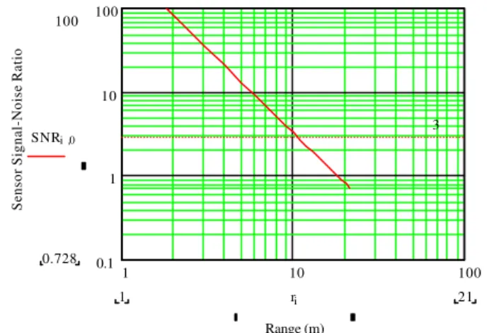
Lambertian diffusing surface model. Figure 17 shows the signal to noise ratio coefficient (SNR=Ilaser/Isun) for the prototype of

Figure 3 where f=100 mm, Plaser =15 mW. Immunity to sun illumination is demonstrated for typical operating range that will

be used during assembly of the Space Station. For longer range, object illumination will not be as critical because unresolved targets and TOF mode of operation will be used.

Figure 16: Spectral irradiance of the Sun. Figure 17: Signal to noise ratio Ilaser/Isun of the prototype of

the laser scanner in triangulation mode (short-medium distances).

Figure 18: Demonstration under sunlight illumination and analysis of worst case scenarios of on-orbits light conditions. This

was accomplished by comparing the tracking while removing the optical interference filter inside the laser scanner head. Solar Irradiance -0.5 0 0.5 1 1.5 2 2.5 0.0 0.2 0.4 0.6 0.8 1.0 1.2 1.4 1.6 1.8 2.0 2.2 2.4 2.6 2.8 3.0 Wavelength (µµm) kW / (m 2 µµ m) Outside Atmosphere Sea Level Black Body Model

1 10 100 0.1 1 10 100 Range (m)

Sensor Signal-Noise Ratio

100 0.728 3 SNRi 0, 21 1 ri

6. CONCLUSION

A 3-D laser scanner system was presented in this paper that demonstrates excellent tracking characteristics for space assembly operations. The laser scanner can be used either in imagery or in tracking modes, using either time-of-flight (TOF) or triangulation methods for range acquisition. The laser scanner uses two high-speed galvanometers and a collimated laser beam to address individual targets on an object. High-resolution pointing and excellent tracking accuracy were obtained using Lissajous scanning patterns.

The laser scanner basic performances, using directly the range data from the measurements have been demonstrated. However, combining these ranging modes with the high pointing accuracy obtained using the Lissajous tracking pattern, and photogrammetric methods (spatial resection), increased accuracy by approximately an order of magnitude was obtained. This combination of ranging techniques makes the laser scanner compatible with the current Space Vision System (SVS) used by NASA. Experimental range stability of 4 mm was obtained for an object at a distance of 10 m from the camera.

An important objective of the 3-D Laser Tracking System, to provide immunity to Sun interference while tracking, was successfully demonstrated both mathematically and experimentally. Worst-case scenario where intensity of the returned laser signal and high intensity gradient illumination created by sunlight and shadows was analyzed. Results have shown that the current prototype, using a 15 mW laser source at 1.5 µm is operational at distances of up to 20 m, in triangulation mode, and can be further increased by using higher laser sources, or the TOF mode of operation.

7. REFERENCES

1. Clair L. Wyatt, “Radiometric system design”, Macmillan Publishing Company, New York, NY, USA

2. G.C. Holst, “Electro-Optical Imaging System Performance,” SPIE Optical Engineering Press, JCD Publishing, Winter Park, FL., 1995.

3. S.G. MacLean, and H.F.L. Pinkney, ``Machine Vision in Space,” Canadian Aeronautics and Space Journal, 39(2), 63-77 (1993).

4. S.G. MacLean, M. Rioux, F. Blais, J. Grodski, P. Milgram, H.F.L. Pinkney, and B.A. Aikenhead, “Vision System Development in a Space Simulation Laboratory,”in Close-Range Photogrammetry Meets Machine Vision, Proc. Soc. Photo-Opt. Instrum. Eng., 1394, 8-15 (1990).

5. F. Blais, J.-A. Beraldin, M. Rioux, R.A. Couvillon, and S.G. MacLean, “Development of a Real-time Tracking Laser Range Scanner for Space Application,” Proceedings Workshop on Computer Vision for Space Applications, Antibes, France, September 22-24, 161-171 (1993).

6. F. Blais, M. Rioux, and S.G. MacLean, “Intelligent, Variable Resolution Laser Scanner for the Space Vision System,” in Acquisition, Tracking, and Pointing V, Proc. Soc. Photo-Opt. Instrum. Eng., 1482, 473-479 (1991).

7. D.G. Laurin, F. Blais, J.-A. Beraldin, and L. Cournoyer, “An eye-safe Imaging and Tracking laser scanner system for space Applications,” Proc. Soc. Photo-Opt. Instrum. Eng. 2748, 168-177 (1996).

8. F. Blais, M. Rioux, and J.-A. Beraldin,”Practical Considerations for a Design of a High Precision 3-D Laser Scanner System,” Proc. Soc. Photo-Opt. Instrum. Eng. 959, 225-246 (1988).

9. J.-A. Beraldin, S.F. El-Hakim, and L. Cournoyer, “Practical Range Camera Calibration,” Proc. Soc. Photo-Opt. Instrum. Eng. 2067, 21-31 (1993).

10. G.H. Suits, “Natural Sources,”Chap.3 in The Infrared Handbook by W.L.Wolfe and G.J. Zissis Editors, ERIM, 1989. 11. K.J. Gaskik,, “Optical Metrology,” 2nd Ed., John Wiley & Sons, West Sussez, England, 1995.

12. Beraldin, J.-A., Blais, F., Rioux, M., Cournoyer, L., Laurin, D., and MacLean, S.G. “Eye-safe digital 3D sensing for space applications”. Opt. Eng. 39(1): 196-211; Jan. 2000.