The sources of hospital cost variability
∗†
Brigitte Dormont
‡and Carine Milcent
§June 24, 2004
Abstract
Hospital heterogeneity is a major issue in defining a reimbursement system. If hospitals are heterogeneous, it is difficult to distinguish which part of the differences in costs is due to cost containment efforts and which part cannot be reduced, because it is due to other unobserved sources of hospital heterogeneity. In this paper, we apply an econometric approach to analyse hospital cost variability. We use a nested three dimensional database (stays-hospitals-years) in order to explore the sources of variation in hospital costs, taking into account unobservable components of hospital cost heterogeneity. The three dimensional structure of our data makes it possible to identify transitory and permanent components of hospital cost heterogeneity. Econometric estimates are performed on a sample of 7,314 stays for acute myocardial infarction (AMI) observed in 36 French public hospitals over the period 1994 to 1997. Transitory unobservable hospital heterogeneity is far from negligible: its estimated standard error is about 50 % of the standard error we estimate for cost variability due to permanent unobservable heterogeneity between hospitals.
JEL classification: C23, H51, I18
Keywords : Hospital costs, moral hazard, unobservable hospital heterogeneity, panel data.
∗We are grateful for the helpful comments of Werner Antweiler of the Faculty of Commerce, University of British Columbia, Alberto Holly, University of Lausanne, Michel Mougeot, University of Besançon, and Isabelle Durand-Zaleski, ANAES. We also thank the participants of the NBER Summer Institute workshop (Boston) for useful comments as well as the participants of the Crest-LEI and of the Delta seminar in Paris, Martin Chalkley and the participants of the twelfth European Workshop on Econometrics and Health Economics (Menorca). We are also grateful to two anonymous referees whose comments improved the paper. This study was funded in part by grants from the DREES (Direction de la Recherche, des Etudes, de l’Evaluation et des Statistiques) of the French Ministry of Labor and Solidarity.
†Corresponding author: Brigitte Dormont Thema UPX, Bâtiment G, 200 avenue de la république 92001 Nanterre
cedex, France. Tel: 00 33 1 40 97 78 36. Fax: 00 33 1 40 97 59 73 . E-mail address : dormont@u-paris10.fr.
‡Thema-CNRS, University of Paris10-Nanterre, France and, IEMS Institut d’Economie et de Management de la
Santé, Lausanne, Switzerland.
§Delta-CNRS, Ecole nationale Supérieure, Paris, France and, IEMS Institut d’Economie et de Management de la
1
Introduction
Large variations in hospital costs are observed in several countries. In the US, the range from the 5th to the 95th percentile of hospital Medicare standardised cost per case was 142 % in 1985 [1]. In France, in 1996, the range from the standardised cost per case in the least expensive public hospital to the standardised cost per case in the most expensive public hospital amounted to 226 % [2].
It is possible to interpret this variability as resulting from inefficiencies between hospitals. In France, many economists incriminate the current reimbursement system of public hospitals. Indeed, the global budget which was implemented in 1983 has led to large disparities in the financial burdens faced by hospitals. One solution would then be to address inefficiencies through an appropriate reimbursement policy, such as a Prospective Payment System per DRG.
In principle, prospective payment provides a strong incentive to keep costs down and avoid inefficiency [3,4]. However, a few years after the implementation of such a system for the Medicare patients in the US, some authors have pointed to the enormous remaining variations in hospitals costs and argue that some portion of hospital cost differences was justifiable [1, 5, 6]. As stated by Newhouse [7,8], reimbursement should not necessarily be fully prospective. One has to take "legitimate" cost heterogeneity into account, in order to avoid the risks of a fully prospective payment system, i.e. patient selection, lower care quality, creaming, skimping and dumping [1,6,8-11].
Analysing hospital cost variability is thus of major importance. It can make it possible to evaluate the relative importance of components of cost variability and to gauge inefficiency and the need for reimbursement policies that address inefficiencies, as opposed to compensating for variability in case-mix. To what extent does inefficiency influence cost variability ? To what extent should patient and hospital heterogeneity be allowed for in a payment system ? Answering these questions requires more knowledge about the sources of variation in hospital costs.
Except for a few cases (such as Kessler and McClellan [25]) the studies about hospital costs use information about average cost at hospital level. For example, the recent panel data studies of Linna [14] and Rosko [19] about Finnish and US hospitals concern two dimensional databases recording observations relative to hospitals-years. We have at our disposal a three dimensional nested database (stays-hospitals-years) that is sufficiently rich to disaggregate the components of
hospital cost variation.
Many studies about hospital costs focus on the issue of efficiency. A common approach is based on the data envelopment analysis [12-15]. Other studies use stochastic frontier models [14,16-19]. Some of them focus on the additional cost due to specific activities of hospitals. For example, Lopez-Casanovas and Saez [20] estimated the extra cost for teaching hospitals in Spain. As stated by Linna [14], most studies of hospital efficiency can be criticized for not having measured output or even case-mix appropriately. In addition, most of the stochastic frontier studies have used cross-sectional data. The use of panel data in efficiency analysis makes it possible to specify the efficiency parameter as a parametric function of time or of explanatory variables [21,22]. Another advantage of panel data, pointed out by Schmidt and Sickles [23], is that they make it possible to avoid distributional assumptions. When inefficiency is assumed to remain constant over time, it can be specified as a hospital’s specific effect, which can be treated as fixed or random. However, one limit of this approach is that it assumes that all unmeasured hospital heterogeneity is due to inefficiency [24].
The purpose of this paper is to explore the sources of hospital cost variability in France. We take advantage of a three dimensional nested database (stays-hospitals-years) of 7,314 stays for acute myocardial infarction observed in 36 French public hospitals over the period 1994 to 1997. Information is recorded at three levels: stays are grouped within hospitals and hospitals are observed over several years. The available information makes it possible to evaluate the respective influences of observable patient characteristics and hospital characteristics on cost variability. In addition, the complex structure of our panel data allows us to identify two components of unexplained cost variability: short term unobserved hospital heterogeneity and permanent unobserved hospital heterogeneity.
The remainder of this article is organized as follows. In section 2, we describe the data, char-acterizing the stays, the observed pathologies, as well as the hospitals in the database. Section 3 defines econometric specifications that make it possible to analyze costs and identify the compo-nents of cost variability. Section 4 presents econometric methods, specification tests and the results of the econometric application. We conclude in section 5.
2
Description of the data
We have at our disposal a sample of 7,314 stays for acute myocardial infraction (AMI) observed in 36 French public hospitals over the period 1994-1997. In France and in the present study, the term ”public hospitals” stands for hospitals belonging to the public sector as well as most of the private-not-for-profit hospitals. In France, public hospitals account for most of the total admissions (2/3 of admissions for AMI). Our sample has been extracted from the PMSI cost database. PMSI stands for the Programme de médicalisation des systèmes d’informations, which collects information about hospital activity. Classification of stays by Diagnosis Related Group (DRG) is performed on the basis of diagnoses and procedures implemented during the stay. Within a prospective payment system, the regulator would define payments for each DRG. In order to obtain a high degree of patient homogeneity in terms of pathologies we selected patients aged at least 40 years with acute myocardial infraction (AMI) as the main diagnosis and grouped in the same DRG: uncomplicated AMI (DRG 179).
For each stay, we have information about the cost of the stay, secondary diagnoses, procedures implemented, entry mode into the hospital (coming from home or transferred from another hospital), discharge mode (return home or transfer), length of stay, age and gender of the inpatient.
The database gives access to rich and detailed information about stays. However, the information about services provided is rather limited. We cannot follow the same inpatient through successive hospital stays. There is no information about the patient’s quality of life after the stay, about readmission just after the observed stay, about infections contracted during the stay. In addition, we have no information about the quality of services provided in terms of comfort or alleviation of pain.
Participation in the cost database program is optional. The number of participating hospitals is limited. They consent to give detailed information about their costs, which means that they have accounting systems which enable them to give such information. Using an exhaustive database of AMI patients with no information about costs, we have carried out a comparative analysis about patient characteristics and procedures implemented. This allows us to consider that our data are representative of AMI stays in French hospitals.
Our panel data exhibit a rather complex structure. Information is recorded at three levels: stays are grouped within hospitals and hospitals are observed over several years. The panel is unbalanced in several dimensions: not only does the number of stays recorded vary across hospitals for a given year but also the length of the observation period varies across hospitals. Basic features of the data are presented below. We first examine stays (the lowest level of observation), then we consider hospitals.
2.1
Patients
Most AMI patients (64.3 %) are grouped in DRG 179 (uncomplicated AMI). Together with drug therapy (aspirin, beta blockers, etc.), uncomplicated AMI patients can receive various treatments such as thrombolytic drugs, cardiac catheterization (hereafter denoted as CATH) and percutaneous transluminal coronary angioplasty (PTCA). Catheterization is a specialized procedure used to view the blood flow to the heart in order to improve the diagnosis. Angioplasty (PTCA) appeared more recently than bypass surgery. It is an alternative, less invasive procedure for improving blood flow in a blocked artery.
In France, the use of an innovative procedure such as catheterization or angioplasty do not lead to classification of a stay into a specific DRG. This is rather different from the US classification, where stays with angioplasty are grouped in a specific DRG (DRG 112). These innovative procedures are most often performed within DRG 179: 76.1 % of CATHs and 82.8 % of PTCAs implemented for AMI patients are implemented within DRG 179. Since they do not lead to a classification of the stay in a specific DRG, these costly procedures would not lead to a specific payment within the context of a prospective payment system. A payment system which does not take these procedures into account would therefore penalise the innovative hospitals which use them and give hospitals incentives to select patients.
Basic features of the data are presented in table 1. Most of the patients are men. They are rather young. 89 % of patients come from home. 64 % of discharges are performed to return home and 36 % are transfers to another hospital. AMI with death are grouped in another DRG (GHM 180). The average death rate for all AMI patients is about 9 %. Catheterization and angioplasty are implemented for, respectively, 38 % and 12 % of stays classified in DRG 179.
2.2
Hospitals
Stays are recorded for 36 hospitals, over the period 1994-1997 (table 2). Not all the hospitals are observed over the whole period.
A sizeable proportion of hospitals never perform catheterization or angioplasty. These proce-dures require specific abilities and high-tech facilities. We have introduced a dummy variable for the innovative hospitals. For a given year, a hospital is considered innovative if it has performed catheterization for at least 2 % of the stays, or at least one angioplasty (with or without stent). On the basis of this definition, 20 hospitals are classified as innovative and these hospitals account for 71.5 % of the recorded stays (table 2).
To complete our database, we have also recorded information about hospital type from the SAE survey (the ”Statistique Annuelle des Etablissements de santé” (SAE) is an annual survey which covers all French public hospitals.). There are three types of hospitals: a CHR (Centre Hospitalier Regional.) is a public teaching hospital which also carries out research; a PRIV is a private not for profit hospital (PRIV hospitals have only recently been regulated through the global budget system and only partially so); PUB refers to other public hospitals. Table 3 shows that all the CHR and most of the PRIV are innovative hospitals.
Other indicators are available in the SAE survey, such as number of beds, occupation rate of beds, diversification of activities within the hospital. However, a lot of missing observations prevent us to carry out a complete descriptive analysis. On a restricted number of observations, we find that CHRs are large hospitals with highly diverse activities. On the other hand, private not for profit hospitals (PRIVs) concentrate their services on a small number of activities.
We tried to find empirical evidence of a link between hospital size (and diversification of activ-ities) and the level of costs, but did not obtain significant results.
Table 4 shows correlation coefficients between hospital type, the dummy variable INNOV and averaged indicators computed at the hospital-year level (95 observations). INNOV indicates that the hospital is innovative and can vary over time: a hospital can be non-innovative one year, and perform high-tech procedures the year after. CHRs are innovative and have a low rate of discharge
through transfer to another hospital. Private not for profit hospitals (PRIV) are characterized by a high rate of use of innovative procedures and a high rate of admission through transfer from another hospital. Other publics hospitals are rather non innovative and are characterized by a small rate of use of innovative procedures. Patient flows towards innovative hospitals appear clearly in (i) the positive correlation coefficients we find between admission rate through transfer and CATH or PTCA rates; (ii) the negative correlation coefficients we find between discharge rate through transfer and CATH rate.
2.3
Costs
2.3.1 Historical context
In France, public hospital budgets have been based on a global budget system for more than ten years, including the period 1994 to 1997 that we study. A complete information system which classifies inpatient stays by DRG has been set up, but a PPS has not been implemented. No real attempt at reform was undertaken from 1994 to 1997 (a gradual introduction of a PPS is planned for 2004). Budgets have no direct link to the actual production of hospitals. Hospitals are managed by conventional salaried administrators and do not keep the gains resulting from cost-reducing efforts. In addition, they are more or less subject to a soft budget constraint. This regulation has led to inequity and inefficiency in the allocation of ressources [26].
In our sample, we have detailed information about costs per stay. These costs result from an activity financed on the basis of a global budget system, as it has been implemented in France.
2.3.2 Average costs
Table 5 gives average costs. The average cost per stay is equal to 4,198 Euros with a standard error of 2,863 Euros. On average, a stay is more costly when an innovative procedure has been implemented. As concerns hospital characteristics, stays are more expensive in teaching and in private not for profit hospitals. The stays are also costlier in innovative hospitals.
3
Econometric specifications
3.1
Specification of the cost function
Our observations are at the individual level of hospital stays. Therefore, our approach is different from papers which evaluate efficiency using data relative to average costs per hospital. A survey of this literature can be found in Linna [14]. A few American studies focus like us on a more disaggregated approach, using data at the patient level [25, 27-29]. However, unlike French data, American data record charges per stay instead of cost per stay.
As stated above, the costs we observe result from activity financed on the basis of a global budget system. Cost variability is therefore influenced by several factors: (i) patient characteristics, (ii) hospital characteristics (infrastructure, economies of scale, economies of scope), (iii) inefficiency (which is more or less possible, depending on the generosity obtained by the hospital manager from the regulator when bargaining for the budget), (iv) care quality (which affects mainly the permanent unobserved heterogeneity).
Let us denote Ci,h, tthe cost of stay i in hospital h during the year t. We consider the following
model :
Ci,h,t= Xi,h,t0 γt+ Wh,t0 α + Q0hλ + a + ct+ ηh− εh,t+ ui,h,t (1)
X0
i,h,trepresents individual patient characteristics, such as cross effects age x gender, admission and
discharge modes, length of stay. The explanatory variables W0
h,t and Q0h are observable hospital
characteristics: the type (teaching, private not for profit or other public hospital), whether the hospital is innovative or non innovative (see the definition of an innovative hospital in section 2.2.), implementation rate of high-tech procedures, rates of admission or discharge through transfer. a is a constant.
We have chosen a linear specification for the cost function. The dependent variable is Ci,h,tand
not Log(Ci,h,t). It is well known that health care expenditures generally have a very asymmetric
distribution. In our case, however, the distribution is truncated on the right because of the selection of stays grouped in DRG 179 (uncomplicated AMI). More costly stays are grouped in other DRGs: complicated AMI or AMI treated by bypass surgery. Therefore, the tests (skewness and kurtosis)
we have carried out on the distribution of Ci,h,t have led us to the conclusion that it is closer to a
normal than to a lognormal distribution.
Given patient characteristics, cost variability can stem from hospital characteristics such as hospital type (CHR, PRIV, PUB) and size, diversification of activities, quality of services provided (performance of innovative procedures, comfort, alleviation of pain), skill level of nurses and doctors, quality of hospital management. Some of these factors are observable, some of them cannot be observed.
The observable characteristics for the patients are the variables X0
i,h,t, and for the hospitals the
variables W0
h,t et Q0h.
3.2
Unobserved hospital heterogeneity
Given the observable characteristics, cost variability depends, in the specification (1), on the term:
ct+ ηh− εh,t+ ui,h,t.
ctis a fixed temporal effect which can be linked to technological progress, the pace of price growth
and the general trend of hospital budgets.
We take into account unobservable patient heterogeneity with the random error term ui,h,t ,
which is assumed to be iid (0, σ2
u). εh,tis a perturbation supposed to be iid (0, σ2ε) and uncorrelated
with ui,h,t.
a) Interpretation of hospital specific effects ηh
Unobservable hospital heterogeneity is specified by hospital specific effects ηh, which can be assumed to be random or fixed.
ηhcan be seen as the result of three components. (i) A productivity parameter that is assumed
to be time-invariant: the hospital’s activity is more or less costly, depending on its infrastructure or on the existence of economies of scale or of scope. (ii) Long term moral hazard: the hospital management can be permanently inefficient. (iii) A term taking into account the time-invariant quality of care services.
The perturbation εh,t is defined as the deviation, ceteris paribus, for a given year, of hospital
h’s cost in relation to its average cost.
εh,t is influenced by omitted variables and measurement errors, which are the ordinary
compo-nents of any perturbation. But measurement errors are likely to be of slight importance. Indeed, εh,tis replicated for each stay in the same hospital h during the same year t. Within this framework,
a measurement error can only come from a systematic error in patient registration, or an error in hospital classification. These two possibilities are unlikely. Indeed, the process of building of the PMSI database, as well as checking of these data by the Ministry of Health, prevent such errors from being replicated systematically.
Let us turn now to the other possible components of εh,t, i.e. the omitted variables. εh,tcan be
seen as the result of two components:
- transitory cost reduction efforts, i.e transitory moral hazard. For instance, the manager can be more or less rigorous when bargaining prices for supplies or for services delivered to the hospital by outside firms.
- Transitory shocks which affect hospital h in a given year t. Indeed, εh,t can be influenced by
transitory shocks such as, for instance, an electrical failure. Notice that these shocks are likely to be observable. In addition, they are rather rare.
In principle, εh,t could also reflect transitory variations in quality. However, the civil servant
status of most employees of public hospitals induces rigidity in the work organization and human resources management. The staff of the public hospitals is assigned to a unit. It cannot be rapidly switched from one unit to another one. Similarly, facilities cannot be modified very quickly, since most decisions are taken by a central public administration. Therefore, changes in care quality do not take place quickly. Given the fact that our data covers only four years, it is not unreasonable to rule out the possibility of significant upgrading or deterioration of quality.
On the whole, εh,tis influenced by transitory moral hazard and transitory shocks. The influence
of the latter is likely to be rather small. However, since we cannot evaluate its magnitude, we cannot ignore it.
4
Estimation and results
4.1
Econometric methods
In the model (1) the hospital specific effects ηhcan be assumed to be random or fixed.
Assuming that ηh is random comes down to assuming that unobserved heterogeneity has an influence on costs only at the level of second order moments (on their variance) and is not correlated with observed characteristics Xi,h,t0 , Wh,t0 and Q0h. One has:
Ci,h,t= Xi,h,t0 γt+ Wh,t0 α + Q0hλ + a + ct+ ηh− εh,t+ ui,h,t
| {z }
vi,h,t
, (2)
with ηh iid (0, σ2 η).
Estimation methods are not straightforward for two reasons: (a) our error component model exhibits a nested (hierarchical) structure since the perturbation is written as: vi,h,t = ηh− εh,t+
ui,h,t; (b) our panel data is unbalanced: not only does the number of stays recorded vary across
hospitals for a given year but also the length of the observation period varies across hospitals. Therefore, our model is different from the unbalanced nested error component model considered by Baltagi, Song and Jung [30]. For our case, Antweiler [31] shows that data cannot be easily moulded into a feasible generalized least squares transformation for OLS estimation and that maximum likelihood estimation (MLE) provides a suitable alternative. Under the assumption of normality, a consistent and efficient estimator is given by this MLE.
One can also assume that ηhis a fixed effect. In this case, the model includes hospital dummies (to estimate the fixed effects ηh) and it is not possible to identify the parameters λ. A consistent and efficient estimator is given by the FGLS applied to the following model:
Ci,h,t= Xi,h,t0 γt+ Wh,t0 α + a + ct+ ηh− εh,t+ ui,h,t
| {z }
ξi,h,t
(3)
4.2
Specification tests
Hospital specific effects ηh take unobservable hospital characteristics (long term moral hazard, infrastructure, care quality) which can be correlated with explanatory variables, into account. For
instance, care quality may be higher in a teaching hospital. In order to test for the independence of ηhand to examine whether hospital specific effects are fixed or random, we have used a specification test which is an extension of the test proposed by [32] for the standard error component model. We assume that a correlation between ηhand the explanatory variables can be written as a regression of the form: ηh = X0
.,h,.π1+ Wh,.0 π2+ βh, where βh is iid (0, σ2β) and assumed to be uncorrelated
with εh,t nor with ui,h,t. In this framework, the independence test of ηh is equivalent to the test
for H0: π1= π2= 0 in the model:
Ci,h,t= Xi,h,t0 γt+ Wh,t0 α + X.,h,.0 π1+ Wh,.0 π2+ a + ct+ βh− εh,t+ ui,h,t
| {z }
ζi,h,t
(4)
This test leads us to reject the hypothesis of independence between ηh and the explanatory variables (table 7’). Therefore, we will prefer model (3) , where ηh is fixed. This model is a standard error component model, with a perturbation equal to −εh,t+ ui,h,t. In this case, feasible
generalized least squares lead to a consistent and asymptotically efficient estimate if εh,t is not
correlated with the explanatory variables. A Hausman test allowed us to validate the hypothesis that the effects εh,tare random and not correlated with the explanatory variables (table 7’).
The tests described above are relevant if the explanatory variables are also uncorrelated with the perturbation ui,h,t. This perturbation reflects patient characteristics which are unobservable for
the econometrician, but can be observed by the doctor and therefore influence the cost of the stay. The explanatory variables are not exogenous if they are correlated with these characteristics. For example, the patient’s preferences or risk adversion can influence the length of the stay. Various Hausman tests have allowed us to validate the hypothesis that the variables X0
i,h,t and Wh,t0 are
exogenous (table 7’). Thus, the model (3) can be consistently estimated by the FGLS.
4.3
Results
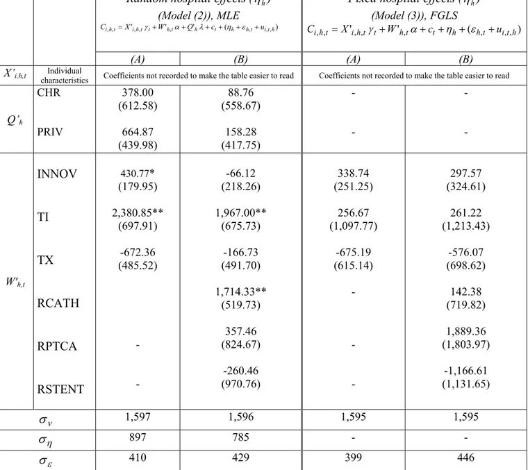
Tables 6, 7 and 7’ present the estimates of the models (2) and (3), and the associated specification tests.
characteristics, were estimated. Model (A) includes indicators close to verifiable characteristics such as hospital type, the variable indicating whether or not the hospital is innovative and average rates of admission and discharge through transfer. Model (B) includes additional variables such as rates of use of innovative procedures, which can be more directly decided on by the hospital.
In order to simplify our presentation, we do not report in table 7 the estimated coefficients of the individual characteristics Xi,h,t0 : indeed the various cross-effects have led to a total number of 32 variables. In order to give an idea of the influence on costs of individual characteristics, of time dummies and of the length of the stay, we report in table 6 the estimation of a simpler model, where cross-effects have been reduced to age x gender effects. The results are quite similar to those of a model comprising all the detailed cross-effects, but they are easier to read. One additional day induces, ceteris paribus, an average additional cost of about 380 Euros. The influence of individual stay characteristics confirms the results generally obtained in studies of stays for acute myocardial infarction. The most costly stays are observed for men. In addition, cost is a decreasing function of age. This latter result may seem surprising because older patients are generally in poorer health. Actually, this is due to the fact that they receive fewer procedures, a fact that is well documented in the medical literature [33,34].
The estimation of an incomplete specification using only individual patient characteristics X0 i,h,t
as explanatory variables reveals that 54.2 % of cost variability can be explained by observable patient heterogeneity. Addition of observable hospital characteristics W0
h,t and Q0hto this specification led
to 68.9 % explained cost variability.
The likelihood ratio test leads us to reject the hypothesis that hospital specific effects ηh are
random. However, the results obtained on both specifications (2) and (3) are worthy of comment. We will then focus on the fixed effects model.
Estimated coefficients of observable hospital characteristics are reported in table 7. The esti-mates of the random effects model show that costs of teaching hospitals (CHR) and costs of private not for profit hospitals (PRIV) do not differ significantly from those of other public hospitals. This result seems rather surprising: the French hospital administration [35] evaluates a 13 % extra cost for teaching hospitals; for teaching hospitals in Spain, Lopez-Casasnovas and Saez [20] estimated, using a rather different method, a significant extra cost of about 9 %. As regards PRIV hospitals,
the French federation of private not for profit hospitals declares that wages are 14 % higher in their sector, inducing 7 % higher costs [36].
On the other hand, the estimate of the random effect model leads to a positive and significant influence (431 Euros) of the capacity to implement innovative procedures (INNOV). Comparing this coefficient to the average cost of a reference AMI stay (4,198 Euros), we obtain an extra cost of 10.2 % for innovative hospitals. This positive effect appears when estimating model A, but becomes negative with the estimation of model B, where rates of use of innovative procedures are part of its explanatory variables. Actually, the negative effect of INNOV is then totally counterbalanced by the positive coefficients of the rates of use. On the whole, being an innovating hospital always induces an extra cost. It is interesting to note that all the teaching hospitals (CHR) in our sample are innovative (table 3). Since the variable CHR has no significant effect, our results therefore mean that hospitals which are innovative are more expensive than others, whether they are CHR or not: the extra cost is more directly linked to innovative activity than to hospital status.
The estimates of the random effect model lead also to a positive effect of the variable TI, indicating that hospitals which accept a high proportion of admissions through transfer have higher costs.
Our estimation procedure allows us to identify two components of the unexplained cost vari-ability: transitory and permanent unobserved hospital heterogeneity. Indeed, the MLE leads to an estimation of ση, the standard error of the hospital specific effects ηh when they are assumed to be
random. And with MLE, we have also estimated σε, the standard error of the perturbation εh,t.
The influence of this transitory unobserved hospital heterogeneity on cost variability is far from negligible: its estimated standard error (410 or 428) is about 50 % of estimated ση (897 or 785).
These results have to be confirmed because, as stated above, the hypothesis of random hospital effects is rejected by our specification test (table 7’). Therefore, we now focus our comments on the estimates of the model where hospital effects ηh are supposed to be fixed.
It is not possible to identify the influence of the constant variables Q0
h from the estimate of the
fixed effects model. In addition, we do not find any significant effect of the variable INNOV, once we have taken permanent differences in average costs into account through the fixed effects.
The fixed hospital effects specification allows us to obtain consistent estimates of the terms ηh, εh,t and of their standard errors ση and σε. The correlation between∧ηh and
∧
εh,t is very small
(-0.001 for models A and B) and not significant. The estimated value of σε is quite similar to the
one estimated by the maximum likelihood estimator: 399 or 446 (models A or B). As regards ση,
one finds estimates which are about 150 Euros larger: 1,057 or 993 (models A or B). This difference can be interpreted as resulting from the effect of hospital type: though unsignificant, this influence was captured by the variables Q0
h in the random effects model. It is integrated in the ηh in the
fixed effects model. The magnitude of cost variability attributable to transitory moral hazard is still sizeable: σεis close to about 50 % of ση.
To get an idea of the magnitude of the standard errors ση and σε, one can compare them to
the standard error of stay costs: 2,863 Euros (for an average cost equal to 4,198 Euros). In graph 1 and 2, we relate the estimated effects∧ηhand∧εh,tto the corresponding average cost per hospital
C.,h,. and average cost per hospital per year C.,h,t (these graphs are shown for model A.). The
observations have been sorted by increasing average cost. Hospital specific effects are linked to average costs per hospital but are far from explaining them entirely (graph 1). Graph 2 illustrates how regular the average costs are, in comparison to transitory unobserved heterogeneity fluctuations. The interpretation is the following. Average costs C.,h,t reflect the allocated budgets. The current
system gives hospitals fairly steady budgets. The gap between budgets and costs reflects transitory shocks or transitory moral hazard.
5
Conclusion
Hospital heterogeneity is a major issue in defining a reimbursement system. If hospitals are hetero-geneous, the purchaser of health services (or the regulator) cannot distinguish between differences in costs due to cost containment efforts and differences which cannot be reduced, because they are due to other unobserved sources of hospital heterogeneity. In this paper, we have applied an econometric approach to explore the sources of variation in hospital costs.
Our estimates allow us to evaluate the influence on cost variability of observable patient and hospital characteristics.
We take hospital heterogeneity into account through observable hospital characteristics and unobserved hospital heterogeneity. Our estimates allow us to identify two components of this unobserved heterogeneity: a time-invariant component and a transitory component.
This study makes it possible to assess the relative weights of the various causes of heterogeneity in the French public hospital costs. As regards observable characteristics, it shows the influence on costs of the use of innovative procedures. Turning to unobservable components of cost vari-ability, our result highlight the magnitude of transitory unobserved heterogeneity. Its estimated standard error is about half of the standard error we estimate for cost variability due to permanent unobservable heterogeneity between hospitals.
If transitory shocks which affect the cost of all the stays in one hospital in a given year are very rare, it is possible to interprete this component as mainly due to transitory moral hazard. Indeed, given the management rules of French public hospitals, transitory variations in quality seem to us unlikely during a rather short period of time.
If this interpretation is correct, a payment system could be designed based on the conjecture that transitory unobserved hospital heterogeneity is entirely due to moral hazard. Such a payment system could induce significant budget savings, given the fact that a sizeable share of cost variability is explained by transitory unobserved hospital heterogeneity. However, this interpretation requires further investigations. One limitation of our results is that we cannot identify the share of transitory unobserved hospital heterogeneity that is due to transitory moral hazard. Access to data over a longer period is required to study this question more thoroughly.
6
References
• 1. Pope, G. Using hospital-specific costs to improve the fairness of prospective reimburse-ment, Journal of Health Economics, 1990, vol 9, n◦3: pp 237-251
2. Coca, E. Hôpital silence ! Les inégalités entre les hôpitaux, Ed. Berger-Levrault, 1998 3. Shleifer, A.. A theory of Yardstick Competition, Rand Journal of Economics, 1985, vol
4. Chalkley, M. and J. M Malcomson. Government purchasing of health services, in: Culyer A.J. and Newhouse J.P. editors, Handbook of Health Economics, 2000, Vol. 1A (North Holland, Amsterdam), Chapter 15, 847-890.
5. Keeler E. B.. What proportion of hospital cost differences is justifiable ?, Journal of Health Economics, 1990 9(3), 359-365.
6. Goodall C. A simple objective method for determining a percent standard in mixed reimbursement systems. Journal of health Economics, 1990, 9(3), pp.253-71.
7. Newhouse J. Frontier estimation: how useful a tool for health economics? Journal of health Economics, 1994, 13: 317-322.
8. Newhouse J. P. Reimbursing health plans and health providers : efficiency in production versus selection, Journal of Economic Literature, 1996. Vol. XXXIV : 1236-1263. 9. Ma, A. C. T.. Health care payment systems: cost and quality incentives, Journal of
Economics and Management Strategy, 1994 , vol 3, n◦1: pp 93-112
10. Ma, A. C. T.. Health care payment systems: cost and quality incentives- Reply, Journal of Economics and Management Strategy, 1998, vol 7, n◦1: pp 139-142
11. Ellis, R. P.. Creaming, Dumping, skimping: Provider competition on the intensive and extensive margins, Journal of Health Economics, 1998, vol 17: pp 537-555
12. Burgess, J. and P. Wilson. Hospital ownership and technical inefficiency, Management Science, 1996, vol 42: pp. 110-123.
13. Magnussen, J. Efficiency measurement and the operationalization of hospital production. Health Services Research, 1996., Vol 31: pp 21-37
14. Linna M. Measuring hospital cost efficiency with panel data models, Health Economics, 1998, 7: pp 415-427.
15. Seiford L. A DEA bibliography (1978-1992). In Data Envelopment Analysis: Theory, Methodology and Applications, Charnes A., Cooper W. Lewin A., Seiford L. (eds). Kluwer Academic Publishers: Dordrecht, 1994; 437-469.
16. Wagstaff A. Estimating efficiency in the hospital sector: a comparison of three statistical cost frontier models, Applied Economics, 1989; Vol.21, pp 659-672
17. Zuckerman, S., J. Hadley and L. Lezzoni. Measuring hosppital efficiency with frontier cost functions. Journal of Health Economics, 1994, Vol 13: pp 255-280.
18. Wagstaff, A. and G. Lopez. Hospital costs in catalonia: a stochastic frontier analysis. Applied Economic Letters, 1996, Vol 3: pp 471-474.
19. Rosko M. D. Cost efficiency of US hospitals: a stochastic frontier approach. Health Economics, 2001, Vol.10 pp 539-551.
20. Lopez-Casasnovas, G. and M. Saez. The impact of teaching Status on Average Costs in Spanish Hospitals, Health Economics, 1999, vol 8, n◦7: pp 641-651
21. Battese G. and Coelli T. Frontier production functions, technical efficiency and panel data: with application to paddy farmers in India. Journal of Productivity Analysis 1992; 3: 153-169.
22. Battese G. and Coelli T. A model for technical efficiency effects in a stochastic frontier production function for panel data. Empirical Economics 1995; 20: 325-332
23. Schmidt, P. and Sickles, R. C. Production frontiers and panel data. Journal of Business and Economic Statistics, 1984; 2: 367-374.
24. Hadley J. and Zuckerman S. The role of efficiency measurement in hospital rate setting. Journal of health Economics, 1994, 13: 335-340.
25. Kessler D. and M. McClellan. The effects of hospital ownership on medical productivity, RAND Journal of Economics, 2002, Vol. 33, n◦3: pp. 488-506.
26. Mougeot M.. Régulation du système de santé, CAE, La Documentation Française, Paris, 1999.
27. McClellan M. Hospital reimbursement incentives : an empirical analysis, Journal of Economics and Management Strategy, 1997, 6(1) : 91-128.
28. McClellan M. and J. Newhouse. The marginal cost-effectiveness of medical technology: A panel instrumental variables approach, Journal of Econometrics, 1997, Vol. 77: pp. 39-64.
29. Meltzer D., J. Chung and A. Basu. Does competition under Medicare Prospective Pay-ment selectively reduce expenditures on high-cost patients?, RAND Journal of
Eco-nomics, 2002, Vol. 33, n◦3: pp. 447-468.
30. Baltagi, B. H., S. H Song. and B. C. Jung. The unbalanced nested error component regression model, Journal of Econometrics, 2001, vol 101: pp 357-381
31. Antweiler, W. Nested random effects estimation in unbalanced panel data, Journal of Econometrics, 2001. vol 101: pp 295-313
32. Mundlack Y.. On the Pooling of Time Series and Cross-Section Data, Econometrica, 1978, Vol 46: pp 69-85
33. Regueiro CR, Gill N, Hart A, Crawshaw L, Hentosz T, Shannon RP. Primary angioplasty in acute myocardial infarction: does age or race matter? J Thromb Thrombolysis. 2003 15(2):119-23.
34. Rathore SS, Mehta RH, Wang Y, Radford MJ, Krumholz HM.Effects of age on the quality of care provided to older patients with acute myocardial infarction. Am J Med. 2003 114(4):307-15.
35. Direction des Hôpitaux de Paris, mission PMSI. Le PMSI, analyse médico-économique de l’activité hospitalière, La lettre d’information hospitalières, 1996.
36. Apparitio, S., A.-M. Brocas and J.-C. Moisdon. La place du PMSI dans l’allocation des ressources en île-de-France, Agence Régional d’Hospitalisation d’île-de-France - Rapport technique, 1999.
37. Baltagi, B. H.. Simultaneous equations with error components, Journal of Econometric, 1981 vol 17 : pp 189-200
Table 1: Patient characteristics
Number of stays Proportion (%)
Gender men 5,400 73.8 women 1,914 26.2 Age 40-64 1,861 25.4 65-74 2,733 37.4 75-84 2,271 31.1 85 and over* 449 6.1 Length of stay one day 439 6.0
between 2 and 7 days 2,460 33.6
between 8 and 14 days 3,234 44.2
over 14 days 1,181 16.2 Admission home 6,493 88.8 Other hospital 821 11.2 Discharge Other hospital 2,612 35.7 home 4,702 64.3 Procedures CATH 2,788 38.1 PTCA 853 11.7 Stent 374 5.1
Cost Database: 7,314 stays, 1994-1997
Table 2: Hospitals of the cost database Years Number of
hospitals innovative Whose hospitals
Number of
stays Share % of stays in innovative hospitals 1994 1995 1996 1997 21 27 17 30 12 16 10 18 1,669 2,028 1,267 2,350 70.2 69.7 78.3 70.5 1994-1997 36 201 7,314 71.5
Cost Database: 7,314 stays, 1994-1997
*: Patients aged of 100 years and over have been removed from our sample.
Table 3 : Innovative and non-innovative hospitals
Innovative Non-innovative Total
(hospitals * years) CHR
(teaching hospital)
PUB (other public hospital)
PRIV (Private not for profit)
9 35 12 0 35 4 9 70 16 Total 56 39 95
Cost Database: 7,314 stays, 1994-1997
Table 4 : Correlation coefficients between average hospital characteristics
INNOV TI TX MLOS MCATH MPTCA MSTENT
CHR 27.0 ns -39.6 19.82 32.3 ns ns
PUB -30.4 -29.9 30.7 ns -58.2 -51.9 -32.9
PRIV ns 45.0 ns ns 43.3 54.5 40.1
INNOV 100 ns -45.1 25.5 73.7 35.7 24.8
95 Hospital * years from the costdatabase; ns: non statistically significant correlation coefficient (P<0.05).
The following variables are recorded in the SAE database or computed for the 95 hospitals * years of the cost database (1994-1997):
CHR: Regional Hospital Center (teaching and research activity) PUB: other public hospital
PRIV: private not for profit hospital.
INNOV: innovative hospital (i.e. having the ability to perform a PTCA or a CATH).
TI: admission rate of patients being transferred from another hospital (average per hospital and per year). TX: discharge rate of patients being transferred to another hospital (average per hospital and per year). MLOS: length of stays (average per hospital and per year).
MCATH: CATH rate (average per hospital and per year).
MPTCA: PTCA rate of patient (average per hospital and per year). MSTENT: STENT rate of patient (average per hospital and per year).
Table 5 : Average costs (Euros)
Average cost (Euros)
Overall mean (standard error) (2,863) 4,198 Men Women 4,141 4,398 40-64 65-74 4,104 4,233 75-84 4,480 85 and over 4,155 With Cath 5,099 With Ptca 5,740 With Stent 5,978 Without procedure 3,666 Teaching hospital (CHR) 5,205
Private not for profit (PRIV) 4,630 Other public hospital (PUB) 3,816
Innovative hospital 4,453
Non-innovative 3,592
Table 6 : Influence on cost of patient characteristics, length of stay and time (Euros)
Estimated coefficient
Age*sex
Man : 40-64 years reference
Man : 65-74 years -221.0**
Man : 75-84 years -540.0**
Man : 85 years and over -1,098.4**
Woman : 40-64 years -396.9**
Woman : 65-74 years -426.3**
Woman : 75-84 years -719.3**
Woman : 85 years and over -1,326.4**
Length of stay 378.2** Time dummies Year 1994 reference Year 1995 260.5* Year 1996 768.6** Year 1997 583.5**
Cost Database: 7,314 stays, 1994-1997
** : the coefficient is significant (1 %), * : the coefficient is significant (5 %).
Estimation by feasible generalized least square (residuals:
−
ε
h,t+
u
i,h,t) for a model with fixed hospital effectη
h.Table 7: Cost function estimates (Euros)
Random
hospital effects
(η
h) (Model (2)), MLE ) ( ' ' ',, , , ,, , ,ht iht t ht h t h ht ith i X W Q c u C = γ + α+ λ+ +η +ε +Fixed hospital effects
(η
h) (Model (3)), FGLS ) ( ' ', , , , ,, , ,ht iht t ht t h ht ith i X W c u C = γ + α+ +η + ε + (A) (B) (A) (B) X’i,h,t characteristics Individual Coefficients not recorded to make the table easier to read Coefficients not recorded to make the table easier to readQ’h CHR PRIV 378.00 (612.58) 664.87 (439.98) 88.76 (558.67) 158.28 (417.75) - - - - W'h,t
INNOV
TI
TX
RCATH
RPTCA
RSTENT
430.77* (179.95) 2,380.85** (697.91) -672.36 (485.52) - - -66.12 (218.26) 1,967.00** (675.73) -166.73 (491.70) 1,714.33** (519.73) 357.46 (824.67) -260.46 (970.76) 338.74 (251.25) 256.67 (1,097.77) -675.19 (615.14) - - - 297.57 (324.61) 261.22 (1,213.43) -576.07 (698.62) 142.38 (719.82) 1,889.36 (1,803.97) -1,166.61 (1,131.65) vσ
1,597 1,596 1,595 1,595 ησ
897 785 - - εσ
410 429 399 446Cost Database: 7,314 stays, 1994-1997
All the estimations have year dummies
** : The coefficient is significant (1 %), *: the coefficient is significant (5 %) CHR: teaching hospital (public)
PRIV: Private, not-for-profit hospital INNOV: innovative hospital
TI: admission rate through transfer for hospital h, in year t TX: discharge rate through transfer for hospital h, in year t
RCATH: rate of in-hospital catheterization use for hospital h, in year t
RPTCA: rate of in-hospital percutaneous transluminal coronary angioplasty use for hospital h, in year t RSTENT: rate of in-hospital stent use for hospital h, in year t
Table 7’: Cost function estimates – Statistics and tests
(A) (B) (A) (B)
Log likelihood
- 44,506.42 - 44,497.11R
2 68.5 68.5Likelihood ratio test
)
(
P
>
χ
2 # (0.000) 7,228 (0.000) 7,246Wald test
)
(
P
>
χ
2 13,005 (0.000) 12,913 (0.000)Likelihood ratio test
for independence ofη
h)
(
P
>
χ
2 67.2 (0.0003) 71.8 (0.0005)Hausman test¤ for
independence of
ε
h,t)
(
P
>
χ
2 30.8 (0.5255)# Significance level.
¤ The usual statistics of the Hausman test eliminates automatically the variables t h
W
'
, . So, there is no difference between the tests on models A and B. This test is equivalent to a test for independence betweenX
'
i,h,t andε
h,t. To test for the exogeneity ofW
'
h,t we have used another Hausman's specification test that compares anestimator that is known to be consistent and efficient under the null and alternative hypotheses (here, the error component two-stage least square estimator, EC2SLS [37] with an estimator which is efficient under the null hypothesis (here, feasible generalized least squares estimator, FGLS). Instruments are the patient demographic characteristics and the fully-interacted of the secondary diagnoses, gender and age of the patient. The test provides evidence that we cannot reject the null hypothesis: the variables
W
'
h,t andX
'
i,h,t.are exogenous.Graph 1:
-2,000 -1,000 0,000 1,000 2,000 3,000 4,000 5,000 6,000 7,000 8,000Average cost per hospital Estimated fixed hospital effect (Model A)
Graph 2:
-1,000 0,000 1,000 2,000 3,000 4,000 5,000 6,000 7,000 8,000Average cost per hospital per year