Assessment of mesoscale eddy parameterizations for
coarse resolution ocean models
by
Mikhail A. Solovev
M.Sc. Moscow State University, Russia (1993)
Submitted in partial fulfillment of the
requirements for the degree of
Doctor of Philosophy
at the
MASSACHUSETTS INSTITUTE OF TECHNOLOGY
and the
WOODS HOLE OCEANOGRAPHIC INSTITUTION
September 1999
@ Mikhail A. Solovev, 1999
The author hereby grants to MIT and to WHOI permission to reproduce
and to distribute copies of this thesis document in whole or in part.
Signature of Author ...
Joint Program in Physical Oceanography
Massachusetts Institute of Technology
Woods Hole Oceanographic Institution
July 23, 1999
Certified by .. .
Paola Malanotte-Rizzoli
Professor
Massachusetts Institute of Technology
) Thesis. Snpervisor
Accepted by ...
W. Brechner Owens
Chairman, Joint Committee for Physical Oceanography
Massachusetts Institute of Technology
Woods
* Institution
Vf
Assessment of mesoscale eddy parameterizations for coarse
resolution ocean models
by
Mikhail A. Solovev
Submitted in partial fulfillment of the requirements for the degree of Doctor of Philosophy at the Massachusetts Institute of Technology
and the Woods Hole Oceanographic Institution July 23, 1999
Abstract
Climate simulation with numerical oceanic models requires a proper parameterization scheme in order to represent the effects of unresolved mesoscale eddies. Even though a number of schemes have been proposed and some have led to improvements in the simulation of the bulk climatological properties, the success of the parameterizations in representing the mesoscale eddies has not been investigated in detail. This thesis examines the role of eddies in a 105-years long basin scale eddy resolving simulation with the MIT General Circulation Model (GCM) forced by idealized wind stress and relaxation to prescribed meridional temperature; this thesis also evaluates the Fickian diffusive, the diabatic Green-Stone (GS) and the quasi-adiabatic Gent-McWilliams (GM) parameterizations in a diagnostic study and a series of coarse resolution experiments with the same model in the same configuration.
The mesoscale eddies in the reference experiment provide a significant contribution to the thermal balance in limited areas of the domain associated with the upper 1000M of the boundary regions. Specifically designed diagnostic tests of the schemes show that the horizontal and vertical components of the parameterized flux are not simultaneously downgradient to the eddy heat flux. The transfer vectors are more closely aligned with the isopycnal surfaces for deeper layers, thus demonstrating the adiabatic nature of the eddy heat flux for deeper layers. The magnitude of the coefficients is estimated to be consistent with traditionally used values. However, the transfer of heat associated with time-dependent motions is identified as a complicated process that cannot be fully explained with any of the local parameterization schemes considered.
The eddy parameterization schemes are implemented in the coarse resolution config-uration with the same model. A series of experiments exploring the schemes' parameter space demonstrate that Fickian diffusion has the least skill in the climatological simu-lations because it overestimates the temperature of the deep ocean and underestimates the total heat transport. The GS and GM schemes perform better in the simulation of
the bulk climatological properties of the reference solution, although the GM scheme in particular produces an ocean that is consistently colder than the reference state. Com-parison of the eddy heat flux divergence with the parameterized divergences for typical parameter values demonstrates that the success of the schemes in the climatological sim-ulation is not related to the representation of the eddy heat flux but to the representation of the overall internal mixing processes.
Thesis Supervisor: Paola Malanotte-Rizzoli Title: Professor
Acknowledgements
First and foremost, my sincere gratitude goes to my advisor, Paola Rizzoli. I greatly appreciate her encouragement, trust and advice in every aspect surrounding my graduate study and the thesis research. I would like to acknowledge the help and support at each stage of the thesis project from the members of my Thesis Committee: Jochem Marotzke, Breck Owens, Mike Spall and Peter Stone. Thanks to Glenn Flierl, the Thesis Defense Chairman, for valuable suggestions about the thesis.
I am indebted to Chris Hill and Alistair Adcroft for their help in mastering the MIT
General Circulation Model; all members of the support staff, especially Linda Meinke, for help with computer systems; Lisa McFarren for reading the final version of the thesis. The financial support for this research was provided by ONR grant number
N00014-98-1-0881, Alliance for Global Sustainability and American Automobile Manufactures
Association.
Grateful thank you and dedications to my parents, Alexei and Galina, and to Kris,
Contents
Abstract
Acknowledgements
1 Introduction
1.1 Motivation . . . .
1.2 Outline of the Thesis . . . .
2 Reference Numerical Experiment
2.1 Introduction ... 2.2 Numerical Model ...
2.2.1 Equations ...
2.2.2 Boundary Conditions . . . .
2.2.3 Domain of the Experiment . . . . .
2.3 Specifications of the Numerical Experiment 2.3.1 Internal Parameters . . . .
2.3.2 External Parameters . . . .
2.3.3 Domain and Discretization . . . . . 2.3.4 Initialization . . . . 2.4 Eddy Resolving Calculation . . . . 2.4.1 Initialization Period . . . . 2.4.2 Spin-up Period . . . . 16 17 23 26 . . . . 26 . . . . 28 . . . . 29 . . . . 31 . . . . 31 . . . . 32 . . . . 32 . . . . 33 . . . . 36 . . . . 38 . . . . 45 . . . . 45 . . . . 46
2.4.3 Data Period . . . . 2.5 Sum m ary . . . . 3 Climatological Analysis 3.1 Introduction . . . . 3.2 Climatological Diagnostics . . . . 3.2.1 Density Structure . . . . 3.2.2 Transport . . . .
3.3 Comparison with the Coarse Resolution Experiments . .
3.3.1 Density Structure . . . .
3.3.2 Transport . . . . 3.4 Conclusions . . . .
4 Eddy Heat Flux and the Thermal Balance
4.1 Introduction . . . . 4.2 Prognostic Equation for Temperature . . . . 4.3 Time-Averaged Temperature Balance . . . . 4.4 Estimation of Terms in the Time-Averaged Temperature
4.4.1 Time Mean and Eddy Terms . . . . 4.4.2 Non-Equilibrium in Thermal State . . . . 4.4.3 Convection . . . . 4.5 Horizontal Averaging . . . . 4.6 Balances in the Time-Averaged Temperature Equation . 4.6.1 Layer 2 . . . . 4.6.2 Upper Layer . . . . 4.6.3 Layer 5 . . . . 4.7 Horizontal and Vertical Distribution of Balances . . . . . 4.8 Geographical Distribution of the Eddy Forcing . . . . 4.9 Divergences of the Time Mean and Eddy Heat Fluxes . .
58 . . . . 58 . . . . 59 . . . . 60 . . . . 67 . . . . 72 . . . . 75 . . . . 82 . . . . 92 94 . . . - - - . . . 94 . . . . 95 . . . . 96 Balance . . . . 98 . . . . 98 . . . . 99 . . . . . . . 106 . . . . . 110 . . . . 116 . . . . 116 . . . . - - 117 . . . . - - - - . 120 . . . . . 123 . . . . 128 . . . . 133 48 55
4.10 Conclusions . . . . 5 Diagnostic Tests of Eddy Heat Flux Parameterization Schemes
5.1 Introduction ... ...
135
136 136
5.2 Vector Decomposition . . . 138
5.2.1 Flux Vectors and Gradients . . . 138
5.2.2 Isopycnal basis . . . 141
5.2.3 Projections of Vectors on the Isopycnal Basis . . . 143
5.3 Tests of Eddy Heat Flux Parameterization Schemes . . . 145
5.3.1 Diabatic Schemes . . . 145
5.3.2 Adiabatic Parameterization Schemes . . . 153
5.4 Evaluation of the Tests . . . 156
5.4.1 Test of Fickian Diffusion . . . 158
5.4.2 Test of Isopycnal Diffusion . . . . 173
5.4.3 Test of the Green-Stone Parameterization Scheme . . . 173
5.4.4 Test of the Gent-McWilliams Parameterization Scheme . . . 182
5.5 Summary of the Tests . . . 188
6 Tests of Parameterization Schemes in Coarse Resolution Experiments 192 6.1 Experimental Set-Up . . . 192
6.1.1 Internal and External Parameters . . . 192
6.1.2 Initialization . . . 193
6.1.3 Execution . . . 194
6.2 Evaluation Criteria . . . 194
6.2.1 Climatological Evaluation . . . 194
6.2.2 Flux Divergence . . . 195
6.3 Coarse Resolution Experiments . . . 197
6.3.1 Fickian Diffusion . . . 197
6.3.3 Gent-McWilliams Parameterization Scheme . . . 222 6.4 Conclusions . . . . 232 7 Conclusions A Data Preprocessing 234 242 245 248 B Computations of Operators in the Thermal Balance
List of Figures
1-1 Northward transport of energy as a function of latitude . . . . 18
1-2 Kinetic energy spectrum for the atmosphere and the oceans . . . . 19
2-1 Forcing functions of the simulations . . . . 35
2-2 Wind stress and its curl in the coarse resolution experiments . . . . 39
2-3 Initial conditions for temperature . . . . 42
2-4 Flow diagnostics of the climatological simulation . . . . 44
2-5 Northward integrated heat transport in the climatological simulation . . 45
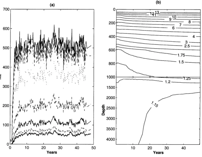
2-6 Spin-up stage of the eddy resolving simulation . . . . 48
2-7 Geographical location of stations . . . . 51
2-8 Data period of the eddy resolving simulation . . . . 53
2-9 Stability of the time average quantities. Station 27. Layer 2 . . . . 54
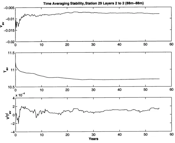
2-10 Stability of the time average quantities. Station 29. Layer 2 . . . . 55
2-11 Barotropic transport in the reference experiment . . . . 57
3-1 Thermal structure of the reference simulation . . . . 62
3-2 Surface heat flux adopted from F. Bryan, 1987 . . . . 63
3-3 Time mean density adopted from B6ning and Budich, 1992 . . . . 65
3-4 Horizontally averaged vertical profile of potential temperature adopted from Robitaille and Weaver, 1995 . . . . 66
3-6 Meridional overturning stream function adopted from Bdning and Budich,
1992 ... ... 69
3-7 Total northward heat transport adopted from B6ning and Budich, 1992 . 71 3-8 Thermal structure of the initial state . . . . 73
3-9 Transport properties of the initial state . . . . 74
3-10 Thermal structure of the coarse resolution experiment . . . . 76
3-11 Transport properties of the coarse resolution experiment . . . . 77
3-12 Zonally averaged temperature difference, the initial state . . . . 78
3-13 Zonally averaged temperature difference, the coarse resolution experiment 79 3-14 Horizontally averaged temperature difference, the initial state and the coarse resolution experiment . . . . 81
3-15 Decomposition of the total integrated northward heat transport, the ref-erence simulation . . . . 88
3-16 Decomposition of the total integrated northward heat transport, the initial state .. .. . . ... ... . ... . .. ... . . - . . . -. . . . .. . 89
3-17 Decomposition of the total integrated northward heat transport, the coarse resolution experiment . . . . 90
4-1 Time series of temperature for three selected locations and depths . . . . 101
4-2 Difference in temperature between the end and the beginning of the sim-ulation . . . .. . . . .. - - - - . . 103
4-3 Contribution to the temperature balance of the local time-drift . . . . . 104
4-4 Contribution to the temperature balance of the local time-drift. Estima-tion from the temperature fields . . . . 105
4-5 Convective events. Station 37 . . . . 108
4-6 Upper layers convection. Station 27 . . . . 109
4-7 Example of stable stratification during the whole length of the simulation. Station 7 . . . - - - . . 111
Noise in the computations of the time mean horizontal divergence . . . .
Effects of moving averaging on the estimation of the time mean horizontal
divergence . . . . . . . 115
4-11 Balances in the temperature equation. Layer 2. Section at 5E Balances in the temperature equation. Layer 2. Section at 15'E Balances in the temperature equation. Layer 1. Section at 5E . Balances in the temperature equation. Layer 1. Section at 150E Balances in the temperature equation. Layer 5. Section at 5E . Balances in the temperature equation. Layer 5. Section at 15'E 3D divergence of the eddy heat flux. Layer 2 . . . . 3D divergence of the eddy heat flux. Layer 2 . . . . 3D divergence of the eddy heat flux. Section at 5E . . . . 3D divergence of the eddy heat flux. Section at 15E . . . . 3D divergencies of the time mean and eddy heat fluxes . . . . . 4-12 4-13 4-14 4-15 4-16 4-17 4-18 4-19 4-20 4-21 5-1 5-2 5-3 5-4 5-5 5-6 5-7 5-8 5-9 5-10 5-11 5-12 5-13 5-14 area . . . . 118 . . . . 119 . . . . 121 . . . . 122 . . . . 124 . . . . 125 . . . . 129 . . . . 130 . . . . 131 . . . . 132 . . . . 134 139 141 143 151 157 159 160 161 162 164 . . . 165 . . . 166 . . . 167 . . . 168 4-9 4-10 113
Definition of the reference point for a flux vector . . . . Local orthonormal isopycnal basis . . . . Projections of vectors on the Isopycnal Angle plane . . . . . Wedge of intstability . . . . Divergence of the eddy heat flux. Layer 2 . . . . Divergence of the eddy heat flux. Layers 1, 2 and 5. Western Test of the Fickian diffusivity on the fine grid. Layer 1 . . .
Test of the Fickian diffusivity on the fine grid. Layer 2 . . .
Test of the Fickian diffusivity on the fine grid. Layer 5 . . .
Vertical component of the eddy heat flux . . . . Distribution of T . . . .. Test of the Fickian diffusivity on the 10 x 10 grid. Layer 1 Test of the Fickian diffusivity on the 10 x 1 grid. Layer 2 Test of the Fickian diffusivity on the 1' x 1' grid. Layer 5
5-15 Test of the Fickian diffusivity on the 20 x 2' grid. Layer 1 . . . . . 5-16 Test of the Fickian diffusivity on the 2' x 20 grid. Layer 2 . . . . . 5-17 Test of the Fickian diffusivity on the 2' x 20 grid. Layer 5 . . . . . 5-18 Divergence of the heat flux associated with Fickian diffusion . . . . 5-19 Projections of i/T' on the isopycnal basis . . . . 5-20 Test of the Green-Stone (GS) parameterization scheme. Layer 1 . . 5-21 Test of the GS parameterization scheme. Layer 2 . . . . 5-22 Test of the GS parameterization scheme. Layer 5 . . . . 5-23 Radius of deformation . . . .
5-24 Mixing coefficient in the GS parameterization scheme . . . .
5-25 Divergence of the heat flux estimated with the GS parameterization 5-26 Test of the Gent-McWilliams (GM) parameterization scheme. Layer 5-27 Test of the GM parameterization scheme. Layer 2 . . . . 5-28 Test of the GM parameterization scheme. Layer 5 . . . . 5-29 Divergence of heat flux estimated with the GM scheme . . . .
Divergence of the eddy heat flux. Layers 1 to 6 . . . .
Horizontally averaged temperature. Fickian Diffusivity Zonally averaged temperature. Fickian Diffusivity . . .
Total heat transport. Fickian Diffusivity . . . . Overturning stream function. Fickian Diffusivity . . . . 3D flux divergence. Experiment FFH5V2 . . . . 3D flux divergence. Experiment FFH1V1 . . . . 3D flux divergence. Experiment FFH5V3 . . . .
Coefficient of the vertical dependence of K . . . ..
Estimation of the GS mixing coefficient . . . . Horizontally averaged temperature. GS scheme . . . .
Zonally averaged temperature. GS scheme . . . . Total heat transport. GS scheme . . . .
. . . 196 . . . . 199 . . . . 201 . . . . 202 . . . . 203 . . . . . 204 . . . 205 . . . . 206 . . . . 210 . . . . 211 . . . . 213 . . . . 214 . . . . 215 . . 169 . . 170 . . 171 . . 174 . . 175 . . 176 . . 177 . . 178 scheme 1 . . 181 182 183 184 186 187 189 6-1 6-2 6-3 6-4 6-5 6-6 6-7 6-8 6-9 6-10 6-11 6-12 6-13
6-14 Overturning stream function. GS scheme . . . .
6-15 Mixing coefficient. Experiment GSA1S1 . . . . 6-16 Flux divergence. Experiment GSA1S1 . . . . 6-17 Mixing coefficients in experiment GSA3S3 . . . . 6-18 Flux divergence. Experiment GSA3S3 . . . . 6-19 Horizontally averaged temperature. GM scheme . . . . 6-20 Zonally averaged temperature. GM scheme . . . . 6-21 Total heat transport. GM scheme . . . . 6-22 Overturning stream function. GM scheme . . . . 6-23 Flux divergence. Experiment AGM5V2 . . . .
6-24 Flux divergence. Experiment AGM7V2 . . . . 6-25 Flux divergence. Experiment AGM5V3 . . . . A-1 Horizontal averaging procedure on the coarse resolution grid
B-1 Definition of the model grid . . . .
. . . 216 . . . 218 . . . 219 . . . 220 . . . 221 . . . 224 . . . 225 . . . 226 . . . 227 . . . 229 . . . 230 . . . 231 . . . 243 . . . 246
List of Tables
2.1 Internal parameters of the reference experiment . . . . 33
2.2 Horizontal dimensions of the domain and horizontal resolution . . . . 37
2.3 Vertical discretization . . . . 37
2.4 Specific parameters of the climatological coarse resolution experiment . . 41
2.5 Data acquisition strategy for the reference experiment . . . . 52
4.1 Range of difference in temperature for 40 stations for each layer . . . . . 102
4.2 Local contribution to the thermal balance. Section 5E . . . . 126
4.3 Local contribution to the thermal balance. Section 15E . . . . 127
5.1 Percent of total area of the Western region with positive diffusivity coeffi-cients. Fine grid . . . . 163
5.2 Percent of total area of the Western region with positive diffusivity coeffi-cients. Averaged over a 10 x 1 box . . . . 165
5.3 Percent of total area of the Western region with positive diffusivity coeffi-cients. Averaged over a 2' x 2' box . . . . 165
5.4 Percent of total area for ratioGS . . . . - - - . . . . 179
5.5 Percent of total area for the GM scheme . . . . 182
6.1 Experiments with Fickian diffusive parameterization . . . . 198
6.2 Experiments with the Green-Stone parameterization . . . 212
Chapter 1
Introduction
Our understanding of climate dynamics and the ability to make forecasts relies to some extent on the numerical models. Complex climate models include the comprehensive representation of physical processes that drive the coupled Atmosphere-Ocean system. Given that a wide range of temporal and spatial scales must be resolved in order to construct a reliable forecast, there are a number of conceptual and technical problems that need to be solved. Although computer technology during the last two decades has sustained an almost exponential growth in computer power and ability to handle large volumes of data, execution of a comprehensive three-dimensional climate model that spans all energetic scales is still not feasible now or in the near future. Thus, current models will have to take into account the important processes on the unresolved scales with the help of parameterization schemes.
One of the most important problems of oceanic modelling on the climatic time scales is poor representation of mesoscale eddies. A number of eddy parameterization schemes have been proposed to represent the transport properties of eddies in complex General Circulation Models (GCMs). Although important, the nature of the eddy momentum flux is not well understood and until recently has been explored only in simple models. The major focus of research in the development of the eddy parameterizations presently aims to represent the eddy flux of tracers, including the active tracers such as temperature
and salinity.
The purpose of this thesis is to explore the proposed eddy heat flux parameterizations in a comprehensive project combining a reference eddy resolving numerical experiment in simplified geometry with a series of coarse resolution experiments using several popular parameterization schemes. The assessment of the schemes in diagnostic and climatolog-ical analyses will address the validity of the parameterization schemes and the poten-tial implementational and conceptual problems in improving the representation of the mesoscale eddies in coarse resolution calculations.
1.1
Motivation
The ocean plays a double role in the climate system. First, it is a giant thermal reservoir with the total mass 270 times greater (Gill, 1982 [24]) and with a heat capacity thousands of times larger than the whole atmosphere. The heat content of only 2.5M of water equals to that of a whole vertical column of air (Gill, 1982 [24]). Second, it transports heat poleward in an amount equal for some latitudes to the atmospheric heat transport (Figure
1-1). Thus, all climatological simulations must reproduce these two major roles correctly.
Nevertheless, experiments with the climatological models tend to have serious prob-lems simulating the oceanic component of the climate. The coupled simulation by Manabe
and Stouffer, 1988 [38] showed that this coupled model can not reproduce the current
climate without some artificial flux adjustment. In addition, the majority of coarse res-olution experiments in a realistic geometry tend to underestimate the northward heat flux by as much as 50%. What are the apparent problems with the oceanic component of these coupled climate models?
One of the potential candidates for this deficiency in the ocean component is the rep-resentation of the unresolved processes. Because of finite resources, numerical simulations with a horizontal grid sufficiently small enough to resolve the most energetic component of the oceanic circulation (Figure 1-2) can not be integrated over the required time to
4 X 2 £0 '" 00 100 200 300 400 500 700 90f Latitude (N)
-2-Figure 1-1: The northward transport of energy, [1015W] as a function of latitude. The
white area is the part transported by the atmosphere and the shaded area the part transported by the ocean. The lower curve denotes the part of the atmospheric transport due to transient eddies. Adopted from VonderHaar and Oort, 1973 [59].
achieve an equilibrium state for the density field. Thus, the mesoscale eddies need to be represented in terms of large-scale quantities. While it is a well-established fact that transports due to transient eddies provide a significant direct contribution to the heat transport by the atmosphere (Figure 1-1, the lower curve), it is still unknown what is the role of eddies in the heat transport by the ocean.
Oceanic mesoscale eddies can either transport heat directly by advecting water in the meridional direction where they exchange heat with the atmosphere, or indirectly by modifying the large-scale density distribution and, respectively, the heat transport. Cox,
1985 [13] and Bdning and Budich, 1992 [4] identified in a series of basin scale experiments
with varying horizontal resolution from 1' down to 1/6' that the explicitly resolved eddy field does not increase the total heat transport but rather modifies the transport by the mean circulation such that the sum of two is a constant. In a recent study by Fanning and
Weaver, 1997 [21], a similar experimental set-up performed for a much longer time and
using lower order horizontal mixing, it was shown that by increasing the resolution and effectively permitting eddies in the model, the total heat transport is indeed increased
5 log E ATMOSPHERE 4- EDDIES -UNRESOLVED log E OCEAN 0-GYRES E -2-UNRESOLVED MOTION -4 -3 -2 -1 0 1 2 3 4 - og10(1xkm-1)
Figure 1-2: Kinetic energy spectrum, [M2 -sec-1], as a function of horizontal wave num-ber, [cyles/KM] , for the atmosphere and the oceans. Adopted from Woods, 1985 [61].
by as much as 50%. This enhancement was observed when the horizontal resolution was
increased from that typical for climate models 4' to 1/4'. In addition, they identified that the increase occurs because of the steady currents, thus demonstrating the importance of the fine resolution in representing the baroclinic gyre component of the total heat transport. The contradiction of these studies suggests that the understanding of the role of eddies in the establishment of climate state of the model is still an open question and requires a consistent representation in the coarse resolution models.
First, it is necessary to perform a climate simulation for millennia time scales as determined by the time scale of adjustment of the thermohaline circulation. Thus, it is
only possible to carry out calculations with a horizontal resolution of a few degrees. The experiment requires a proper parameterization of the effects of time-dependent motions on the transport of properties. All of coarse resolution experiments carried out to date employ one of the proposed eddy heat flux parameterization schemes.
Traditionally, the transfer of heat by mesoscale eddies was assumed to occur in the opposite direction to the gradient of the time mean temperature distribution. The dif-fusive or the Fickian scheme, named after the nineteenth-century German physiologist, Adolf Fick, has been extensively used in ocean modelling (e.g., Sarmiento and K. Bryan,
1982 [49], F. Bryan, 1987 [7]). The scheme assumes that the mesoscale eddies act to
decrease the local gradients of temperature.
The representation of eddy transport as the transfer of heat by eddies excited by baroclinic instability was proposed for the zonally averaged modelling of the atmospheric flows by Green, 1970 [26] and Stone, 1972 [55] and adopted for the potential vorticity flux by Marshall, 1981 [41] in a study of a zonally averaged model of the Antarctic Circumpolar current. The schemes based on a similar concept had a considerable success in the atmospheric modelling (e.g., Stone and Yao, 1990 [56]). So far, the scheme has not been implemented in a primitive equation oceanic GCM.
One of the recently proposed eddy heat flux parameterization schemes is based on a set of different assumptions. While the schemes mentioned earlier rely on the diabatic eddy transfer, the Gent-McWilliams scheme (Gent and Mc Williams, 1990 [23]) represents the eddy heat flux by a quasi-adiabatic process similar to Stokes drift. A non-divergent velocity is added to the time mean Eulerian flow forming a modified advective velocity. The scheme is based on the transformed Eulerian-mean equations originally formulated in atmospheric modelling (Andrews and McIntyre, 1976 [1]; Plumb and Mahlman, 1987 [45]). Following its implementation in the framework of a coarse resolution GCM
(Dan-abasoglu et al., 1994 [15]), the scheme is very popular today and is implemented in the
majority of the primitive equation oceanic GCMs. The most attractive part of the scheme is its quasi-adiabatic nature, as the largest part of the ocean is essentially adiabatic and
mixing occurs predominantly in the isopycnal direction.
While the more sophisticated schemes provide some improvements in the simulation of the climatological state of the ocean compared to a simple Fickian diffusion (Danabasoglu
et al., 1994 [15]; Duffy et al., 1997 [17]; England and Hirst, 1997 [20]), it has not been
demonstrated that the improvements are indeed a result of better representation of the eddies. This important question is the major goal of this thesis project.
The published studies in the area of the assessment of the parameterization schemes can be divided into three major groups. The first group evaluates the schemes in process models. The physical mechanism underlying the parameterization is being reproduced in some framework as the conceptual modelling. The second type of experiments deals with eddy resolving simulations that allow the direct evaluation of necessary fluxes and components of the scheme, thus providing the most consistent evaluation. The third group contains a variety of coarse resolution experiments that can only identify some improvements in the representation of bulk climatological properties. By design, the coarse resolution experiments do not contain explicit information about eddies.
When evaluating a scheme in the framework of a process model, the experimental set-up is the closest reproduction of the physical model originally used for the scheme's development. Therefore, the majority of studies (Marshall, 1981 [41]; Lee et al., 1997
[35]; Visbeck et al., 1997 [58]; Killworth, 1998 [33]; Gille and Davis, 1999 [25]; Treguier,
1999 [57]) consider either zonally averaged or channel model configurations. By
con-struction, this set-up is the oceanic analog of the atmospheric models; thus, the relative success of the schemes in the atmospheric modelling is usually repeated here. These studies investigate use of the parameterization schemes in the ocean regions where in-deed the flow can be approximated by a periodic channel model, such as the Antarctic Circumpolar current. On the other hand the conclusions of these studies may not be valid in the areas where the flow is intrinsically three-dimensional, such as western boundary currents and gyre circulations.
The only experimental set-up that allows the direct evaluation of the eddy heat flux properties is the framework of eddy resolving calculations with a GCM. Only in these experiments a realistic eddy representation can be obtained with the minimum of sim-plifications and the eddy heat flux can be evaluated directly from the simulated data. In addition, all of the details of the parameterization schemes can also be evaluated from the numerical data. Unfortunately, because of the computational difficulties, there is a limited number of such large-scale calculations performed so far. Among the most widely analyzed are the idealized simulation of the North Atlantic (Cox, 1985 [13]; Bdning and
Budich, 1992 [4]); an eddy resolving model simulation of the southern ocean (FRAM Group, 1991 [22]); a realistic simulation of the North Atlantic ocean by the Commu-nity Modelling Effort (CME) group, 1992-1996 ([5], [6]); and a Global Eddy Resolving
model simulation (Semtner and Chervin, 1992 [51]). The primary goals of the exper-iments were the reproduction of the observed features of the ocean general circulation and the most basic eddy activity. The evaluation of the eddy parameterization schemes was not explored. In addition, the length of the experiments was too short, measured in few years (e.g., the individual runs in CME experiments were about 5 years long); thus, the resulting eddy statistics were potentially not stable. Moreover, some of the information required for the evaluation of the eddy parameterization schemes were not collected; for example, in some of the CME experiments the required flux of salinity was not accumulated, so the buoyancy flux was estimated on the basis of the T-S relation. The only study published to date that has attempted to infer the quality of eddy pa-rameterizations from a large-scale eddy resolving simulation is by Rix and Willibrand,
1996 [47] in which the mixing coefficient corresponding to the Gent-McWilliams scheme
is identified of 103 [M2
-sec-1]. However, they did not succeed in describing the spatial patterns of the mixing nor did they assess the quality of the scheme that was due to the insufficient length of the integration.
The coarse resolution experiments simulating aspects of ocean climate are less compu-tationally intensive. Thus, there is a large body of research addressing the climatological
properties of these solutions: total heat transport, strength and structure of the over-turning cell, water mass properties (e.g. Sarmiento and Bryan, 1982 [50]; F. Bryan,
1987 [7]; Danabasoglu et al., 1994 [15]; England, 1995 [19]; Robitaille and Weaver, 1995
[48]; Duffy et al., 1997 [17]). All of these experiments use one of the proposed parame-terization schemes so they can only evaluate how well the bulk climatological properties are being reproduced compared with observations (Levitus, 1982 [36] and 1994 [37]). These experiments can not compare the implied divergence of the parameterized flux with the observations, as the Levitus climatology does not provide observations suitable to evaluate the eddy heat flux and its divergence.
1.2
Outline of the Thesis
The thesis examines the proposed eddy heat flux parameterization schemes in a com-prehensive numerical experiment. The study includes two major parts. The first part addresses the eddy resolving simulation providing necessary numerical data for the esti-mation of the local properties of the parameterizations. The second part of the project deals with the implementation of the schemes in the coarse resolution experiments and the assessment of their skills. All of the simulations are performed with the same numeri-cal model in the same experimental set-up, thus providing a consistent framework for the analysis. Chapters 2, 3, 4 and 5 consider the eddy resolving simulation and present a di-agnostic evaluation of the eddy heat flux parameterization schemes. Chapter 6 addresses the assessment of the schemes in the coarse resolution experiments.
The reference eddy resolving experiment is described in Chapter 2. A necessary description of the MIT GCM is presented at the beginning of the chapter followed by a detailed description of the fine resolution experiment. The major criteria for a successful eddy resolving simulation are stated in the following section. The chapter presents a detailed description of the model's forcing, internal and external parameters. The model is initialized with a climatology obtained with a coarse resolution experiment for typical
values of internal parameters. The evolution of the eddy resolving simulation is presented in the last section of the chapter by analyzing the time series of horizontal kinetic energy and average layers' temperature.
Chapter 3 presents the climatological analysis of the reference experiment by evalu-ating major climatological properties of the simulation. The purpose of the chapter is to demonstrate improvements in the simulated climatological state introduced by explicit representation of the mesoscale processes. The thermal structure of the solution, the total heat transport and the main meridional overturning cell are compared with some published studies and with two coarse resolution experiments. The improved climatol-ogy is a basis of the subsequent comparisons with the coarse resolution experiment using different eddy heat flux parameterization schemes.
The role of mesoscale eddies in the time-averaged thermal balance is evaluated in Chapter 4. The analysis concentrates on a series of meridional cross-sections through the depth of the main thermocline by plotting various terms contributing to the thermal balance. It identifies the areas of the domain where eddies are important by estimating the eddy heat flux divergence and comparing its magnitude to the other terms of the equation. In the western mid-latitudinal area, where the eddy heat flux divergence is the largest, the diagnostic analysis of the eddy heat flux parameterizations is performed and presented in the following chapter.
The detailed properties of the Fickian, the Green-Stone and the Gent-McWilliams schemes are studied in Chapter 5. After the description of the isopycnal framework specifically designed for the diagnostic assessment of the schemes, the three considered parameterizations are analyzed. The diagnostic tests of the parameterization schemes are developed according to the physical mechanisms underlying each of them and evaluated in the following sections. For a typical values of the specific parameters the local divergence of the parameterized flux are computed and compared with the eddy heat flux divergence. The comparison allows evaluation of the schemes' skills in reproducing the geographical distribution of the eddy forcing in the thermal balance.
Chapter 6 evaluates the eddy parameterization schemes in a series of coarse resolution experiments. The simulations are designed in the same framework as the reference ex-periment. The Green-Stone parameterization scheme is implemented in the MIT GCM. The other two schemes are part of the model's code. First, the climatological analysis is performed for the experiments by testing the schemes' skills in reproducing the bulk climatological quantities of the reference simulation. Second, the implied divergence of parameterized flux is evaluated for the best performing experiments and then compared with the divergence of the eddy heat flux of the reference calculation averaged on the grid of the coarse resolution experiments. The analysis helps to answer the question of whether the improvements in the climatological simulations with some of the eddy heat
flux parameterization schemes can be actually attributed to the correct representation of mesoscale eddies.
Chapter 2
Reference Numerical Experiment
This chapter presents the experimental set-up of the project. Due to the importance of the high-resolution numerical experiment, which I will call the "reference" experiment,
I provide a comprehensive description. In the following sections I present the numerical
model and all the successive steps required for the execution of the reference simulation.
2.1
Introduction
The research project is based upon two major parts: a reference fine resolution simula-tion and a number of coarse resolusimula-tion experiments employing different eddy heat flux parameterization schemes. The reference fine resolution calculation is an eddy resolving simulation of a numerical model of a basin scale ocean forced by climatological fluxes. The calculation is carried out starting from a prescribed initial conditions and letting the model evolve until an energetic mesoscale eddy field is developed.
The problem in carrying out such an experiment lies in the length of computational time required for an eddy resolving ocean model to reach a fully equilibrated state. It is well known that the adjustment process of the deep ocean thermal state is controlled in most areas of the domain by advection. This process is very slow below the main thermocline, so it requires thousands of years to reach an overall statistical steady state.
Until that time the model deep circulation preserves the memory of the initial state. The situation is different for the upper ocean, where there is a shorter adjustment time due to faster advective time scale of 0 (10years) and the presence of faster propagating planetary and other waves. These two different adjustment time scales require a mechanism to accelerate the convergence of the integration.
There are two ways which can be used to accomplish this task. The first is the initialization of the model with a field that is close to the expected final steady state. The second is the distorted physics approach (Bryan, 1984 [10]) in which two different time steps are used. The shorter one is for the dynamical variables, the longer for the
thermodynamical variables. The method distorts the physics of the instantaneous state while converging, with some limitations, to the true final steady state.
The majority of ocean climate models use a combination of both methods. They are usually initialized with some a priori known climatology for the density field. Subse-quently, the integration of the models employes small time step for the dynamic variables, of the order of an hour, and a much larger time step for the thermodynamical variables, of the order of a day. There are some further variations, such as an even larger time step for the deeper layers. Overall, this method works only if the final state of the model is truly steady, and is appropriate for coarse resolution simulations. It is not correct to em-ploy this method for eddy resolving models due to the presence of mesoscale variability, in which a "truly" steady state
(-
( ... ) = 0 for all variables) does not exist.The goal of the experiment is to simulate the mesoscale motions and how they in-fluence the climatological state of the model ocean; thus, it is inappropriate to use the distorted physics approach. To accelerate the convergence to the statistical steady state I initialize the experiment with a carefully simulated climatology. In the following sections I present the detailed description of the initialization procedure.
The set of parameters and integration procedures define the solution of the numerical model. The steps in the process following the initialization are the spin-up and the actual
solution of the model's equation, that I call the data period.
2.2
Numerical Model
The model used is the MIT General Circulation Model (MIT GCM). The complete description of this model can be found in Marshall et. al (1997a [43], 1997b [42]). In this section I present a short description of the model that is relevant to my experiment.
The MIT GCM solves Navier Stokes equations in a very general set-up. It can be used for simulations of three-dimensional turbulent flows in basins of varying sizes and shapes: from the symmetrical laboratory tank experiments to the global ocean with realistic profiles of coast line and bottom topography. The model differs from other GCMs mainly by the flexibility of its numerical algorithm, both in terms of formulation and the method of numerical solution. It is possible to use the model in the non-hydrostatic mode; therefore, it can simulate ocean convection and processes occurring in very fine scales such as three-dimensional flows in laboratory tanks. For the larger scale
flows, it can be switched to the hydrostatic formulation, that significantly simplifies the
calculations.
The original formulation of the model has been designed specifically for the calcu-lations on the massive parallel computer Connection Machine (CM-5). The complexity of the parallel implementation of the numerical algorithm is offset by the significant im-provement in the speed of execution (Hill and Marshall, 1995 [29]). Unfortunately the
CM-5 computer is no longer available. I performed the reference fine resolution
experi-ment from February 1997 to March 1998, when there were still available computers. The model is formulated in the finite volume discretization scheme using height as the vertical coordinate. Time-stepping is performed through the quasi-second-order Adams-Bashforth scheme. The model is prognostic in some variables and diagnostic in others.
dynamical equations are transformed into an elliptic equation for pressure, followed by the prognostic time-stepping for the horizontal components of velocity. The next step is the diagnostic calculation of the vertical component of velocity through the non-divergence of the velocity field. The last step is the prognostic calculation of temperature and salinity.
All of the above calculations take into account the finite volume configuration of the grid
and the requirements for time-stepping. For the compete formulation of the numerical algorithm see Marshall et. al (1997a [43], 1997b [42]).
2.2.1
Equations
The general form of the MIT GCM belongs to a class of primitive equation ocean models. It solves Navier-Stokes equations of motion
ath = G(21 - V)P .1
--
= Gw
a
at
' Vz' continuity V -V-4= 0, (2.2) heat aTat
T ' 23 saltas
= Gs, (2.4)at
talking into account the equation of state
p = p (T, S, p) , (2.5)
where ' = (Ba, w) is the three-dimensional velocity, subscript h means horizontal
GV = (G, G,, G,) represents the forcing terms for the dynamical variables, GT and
Gs are the forcing of the temperature and salt equations. The forcing include both the
internal dynamical and thermodynamical mechanisms (inertial, Coriolis, metric, gravi-tational, dissipation) and external forcing due to the interaction with the surrounding environment, such as the atmosphere.
In the reference experiment, the equations (2.1) - (2.5) are simplified according to the
following assumptions:
" Salinity is fixed at So = 350/00; thus, Gs = 0,
" The equation of state is linear p = po - (1 - aT + 3So), where a is the thermal
expansion coefficient,
#
is the coefficient of saline contraction," The hydrostatic approximation is used.
The resulting system of equation in the spherical planetary coordinate system (A,
#,
r)has the following form
Ou 1 0p UVtan#
- a cos A - - VU + a + 2v sin # + F, (2.6a)
v 1 Op u2 tan# - =- - 2Qu sin # + Fv (2.6b) at a0# a 0 -g - -, (2.6c) V - = 0, (2.6d) OT = -V -(v-T)+ F, (2.6e) - = 0, (2.6f)
at
where p = - is the perturbation pressure, i.e. the ratio of the deviation of pressure from
PO
the resting hydrostatically balanced ocean to the reference density; a is the radius of the Earth.
2.2.2
Boundary Conditions
The set of boundary conditions for the large-scale ocean simulation is the following:
" No flow is allowed through the boundaries, V - n' = 0, where n is the normal vector
to the boundary,
* The surface of the ocean is a rigid lid; thus, all fast surface gravity waves are filtered
out, wl_= = 0,
* The tangental velocity component is zero, or no-slip boundary conditions are used at side walls, AI, = 0,
* A constant drag is used at the bottom, z=Hz ~ AB UzH
" No diffusive flux of heat and salt are allowed normal to the solid boundaries,
K,- (T, S) = 0,
" The wind stress at the surface is constant in time, KV- (u, v)|zO 8Z ZO 7 =
g
(r", rO) Pz=O," The heat flux at the surface is set by the relaxation towards an apparent
at-mospheric temperature profile,
* No fresh water flux is allowed through the surface, Ks.S|, _= 0.
2.2.3
Domain of the Experiment
The spherical domain of the experiment extends for a few degrees north of the equator to the polar ocean. The longitudinal extent of the basin is 360 , which roughly corresponds to the width of the midlatitudinal part of the Atlantic ocean. The coast lines are straight, the assumptions simplifying the computations and formulation of the boundary conditions. The bottom of the model ocean is flat.
2.3
Specifications of the Numerical Experiment
The continuous Navier Stokes equations (2.1)-(2.5) describe the behavior of all hydrody-namical systems. The choice of parameters makes the experiment a unique one. I divide the total number of the required parameters into two sets. The first set contains the internal parameters such as diffusivity and viscosity coefficients. The second set contains external parameters, which are independent of the particular numerical representation such as the atmospheric forcings.
2.3.1
Internal Parameters
The main criteria for the choice of sub-grid mixing parameters is the necessity for the solution to support the process of baroclinic instability and the associated formation of mesoscale eddies. The forcing terms of (2.6) (Ft, F, and FT) depend on the internal parameters. The horizontal sub-grid mixing is chosen to be biharmonic. It allows the development of small-scale horizontal motions. The mechanical energy input to the model ocean is removed with the help of bottom drug, a linear function acting on the zonal component of velocity. In a series of preliminary experiments with the model testing the sensitivities to values of internal parameters it was identified that it is not necessary to add the bottom drag for the meridional component of velocity. The magnitude of the zonal bottom drag AB is a constant value everywhere in the domain. It represents the moderate roughness of the observed bottom topography. The form of the forcing terms depending on the internal parameters is the following
F. = Kv.Uzz - Kvbh A2
- AB UzH,
F, = KvwVzz - KvbhA 2V
FT = KTwTzz - KTbhA2T + QTK| O,
Table 2.1: Internal parameters of the reference experiment
- horizontal biharmonic diffusivity, KT - vertical Laplacian diffusivity and QTL,=o-
ex-ternal forcing for temperature in the form of relaxation to some prescribed temperature profile.
The simplest form of the equation of state used in the experiment is a linear function of temperature. Effects of changes in salinity are neglected by keeping it constant through the whole length of the integration, S = 350/00. This value represents an average ocean salinity.
The values of the coefficients are given in Table 2.1.
2.3.2
External Parameters
The sources of energy for the model ocean are the wind stress acting at the surface, and thermal forcing, i.e. the relaxation to an apparent atmosphere for the upper layer. Both components of the forcing are constant in time and vary only meridionally. They represent an approximation to the climatological conditions in the northern hemisphere. The profiles of the forcing are similar to the functions that were widely used in coarse resolution climate simulations (Bryan, 1987 [7], Marotzke and Willebrand, 1991 [40]).
The model is forced through the direct interaction with atmosphere. It exchanges momentum through the action of wind on the surface. The density structure is modified
The shape of the wind stress profile (Figure 2-1(a)) captures the major features of the observed zonally averaged wind stress. Its curl supports the formation of three major wind-driven gyres: the subtropical and subpolar circulations and a tropical gyre maintaining the horizontal circulation in the vicinity of the southernmost boundary. The profile is slightly non-symmetrical with respect to the mid-latitude line of the zero wind stress curl.
The thermal forcing acts on the surface of the ocean. The upper layer of the model ocean is in thermal equilibrium with an apparent atmospheric temperature (Haney, 1971
[28]). The profile of the temperature (Figure 2-1(b)) is a simple sinusoidal function of
latitude:
1 1 (18
Ta = (TE +TP) + (TE - TP)cos - I,
2 2 7
where the equator temperature is TE= 270C and the polar one is TP 0 C. The
corresponding heat flux into the ocean is
H POC(T - T
TD
where C the specific heat of water, 7D the relaxation constant and Ahi the upper layer thickness. The relaxation constant is chosen to be 30 days, equivalent for the upper layer of 50M to a heat flux of about 70 [ W -M- 2] for 1C difference between the upper layer of the model and the apparent atmospheric temperature. Although this value is about two times larger than the standard value estimated by Haney, it provides a reasonable diabatic forcing in the energetic parts of the basin. The expected equivalent surface heat flux is about 300[ W . M-2] for the areas where the deviation of surface layer isotherms from the apparent atmospheric temperature the largest.
1ON 20N 30N 40N 50N 60N Latitude O cc C-CL E I-a. 0. 1ON 20N 30N 40N Latitude Figure 2-1: wind stress
Forcing of the model as functions of latitude: (a) wind stress, [N - M-2] and curl, 10-5 [N .M- 3], (b) apparent atmospheric temperature, [0C].
0.2 0.15 0.1 0.05 0 -0.05 -0.1 -0.15 50N 60N
2.3.3
Domain and Discretization
Horizontal Dimensions
The northern Atlantic ocean is mimicked by the idealized model configuration. In the
northern Atlantic the ocean gains heat in the tropical and subtropical areas and loses heat in the Polar one. When it loses heat to the atmosphere in the northern areas vertical convection occurs and to maintain a stable state heat must be transported from the southern to the northern areas. The basin scale wind-driven circulation further modifies the transport. These processes represent a general oceanic contribution to the climate system and must be represented in the climate simulation.
The numerical domain must comprise all of the above areas in meridional direction. That is, it must span at least one hemisphere. In the zonal direction, the major features of the wind-driven general circulation are reproduced: quiescent interior of mid-latitude gyres, fast western boundary currents and tropical circulation. The breaking of the geostrophic balance right at the equator requires a very small time step to overcome nu-merical instabilities, thus making the whole simulation more computationally expensive. In order to keep the time step reasonably large it was decided to move the southern boundary to 4'N. The northern boundary is located approximately at the area of the possible ice formation at 64'N.
The selection of horizontal discretization is mainly due to two factors. The satisfac-tory simulation of eddies requires the horizontal resolution to be small compared to the radius of deformation since I expect that the mesoscale eddies are the result of baroclinic instability. The definition of the radius of deformation I use is connected with the local quasi-geostrophic approximation. The radius of deformation varies in magnitude with the location in the ocean. The reference value for the mid-latitude ocean is of the order of 50 kilometers. It is smaller in the northern parts and larger for the southern areas due to the increase in the stability of the vertical stratification for the lower latitudes and the decrease in the value of the Coriolis parameter. On the other hand, the smaller
Dimension Degrees min, Km max, Km mean, Km Lx 00E - 360E 1763.5 3970.0 3156.7 LY 40N - 640N 6648.4 6648.4 6648.4 Resolution AX 0.20 9.8 22.2 17.6 AY 0.20 22.4 22.4 22.4
Table 2.2: Horizontal dimensions of the domain and horizontal resolution
Layer 1 2 3 4 5 6 7 8 9 10 11 12 13 14 15
Thickness, M 50 75 100 125 150 200 250 300 400 450 450 500 500 500 500
Mid-depth, M 25 88 175 288 425 600 825 1100 1450 1880 2320 2780 3250 3750 4250
Table 2.3: Vertical discretization
the horizontal resolution the higher the requirements for the computer resources. For the most powerful computers available today, it is impossible to perform a climate simulation on basin scales with the resolution of the order of a fraction of the radius of deformation. Thus, I choose the horizontal resolution to be 0.2'. It is uniform in both meridional and zonal directions. This value is smaller than the radius of deformation in the most areas of the model domain, except some local marginally stable deep convective regions, and at the same time given the appropriate closure coefficients allows the simulation of the mesoscale motions.
The horizontal dimensions and resolution are given in the Table 2.2. The following notations are used in the table: L_ and L. - West-East and South-North dimensions of the basin, Ax and A, - the corresponding horizontal resolution.
Vertical Dimension
The vertical structure of the flow has a non-uniform distribution. The numerical algo-rithm allows one to choose vertical layers of varying thickness. The largest number of layers spans the upper part of the water column, in and above the main thermocline. The deep ocean is represented with a small number of thick layers. Table 2.3 shows the vertical discretization.
The size and discretization of the model ocean domain are comparable to those for the basin scale pioneering eddy resolving simulation by Cox, 1985 [13] and the North Atlantic simulations by the "community modelling effort" (CME) of the World Ocean Circulation Experiment (WOCE) Bryan and Holland, 1989 [8], B6ning and Budich, 1992
[4], Bdning et. al, 1995 [6], 1996 [3].
2.3.4
Initialization
The solution method of the numerical model is time-stepping from an initial state until the model reaches a statistical steady state. This final state is characterized by a balance between the input of energy and dissipation and the generation of eddies and their decay. Due to the non-linear nature of the dynamical equations, there is no guarantee in the uniqueness of the final state. Unfortunately, the modern computational resources do not
allow to perform an ensemble of fine resolution experiments to explore the uniqueness of a final state. Thus, it is important to have some a priori knowledge about the nature of expected final state, so the initial state can be chosen in its vicinity and the solution converges within the limits of the projects resources. In realistic simulations the initial state is usually an observed climatology, compiled from oceanic observations. The most popular data set is the atlas by Levitus, see e.g. Levitus, 1982 [36], [37].
The reference experiment is idealized, with straight coast line and flat bottom topog-raphy. There are two ways to carry out the initialization. One is the initialization with some transformed version of the Levitus climatology. The other is a preliminary simu-lation of an artificial climatology obtained by performing a coarse resolution simusimu-lation. In the latter case the parameters of climatological simulation can be chosen in such a way as to allow for a unique steady solution. The linear equation of state and constant salinity with the combination of large mixing coefficients guarantees the uniqueness of the climatological simulation (Marotzke and Willebrand, 1991 [40]). The final state of the calculation is interpolated on the fine grid of the eddy resolving simulation.
0.2 0.15 F -0.1 F 0.05 F--0.05 k -0.1 H-Coarse resolution 1ON 20N 30N 40N 50N 60N Latitude
Figure 2-2: Wind stress, [N -M-2] , and wind stress curl, 10-' [N -M-3], in the coarse
resolution experiment simulating the initial conditions for the reference experiment.
39 Stress - - Curl r .. ,... . . .. . . /-- -. .. ... .... .
![Figure 2-2: Wind stress, [N - M- 2 ] , and wind stress curl, 10-' [N - M- 3 ], in the coarse resolution experiment simulating the initial conditions for the reference experiment.](https://thumb-eu.123doks.com/thumbv2/123doknet/14107611.466243/39.918.244.662.250.848/figure-resolution-experiment-simulating-initial-conditions-reference-experiment.webp)


![Figure 2-11: Barotropic transport, [Sv] in the reference experiment averaged over 55 years.](https://thumb-eu.123doks.com/thumbv2/123doknet/14107611.466243/57.918.167.760.135.961/figure-barotropic-transport-sv-reference-experiment-averaged-years.webp)
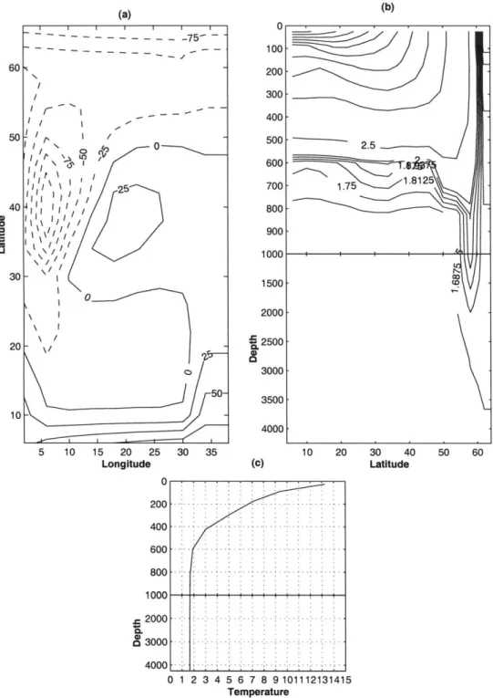
![Figure 3-1: Thermal structure of the reference simulation: (a) surface heat flux, [W - M- 2 ]; (b) zonally averaged temperature, [SC], stretched upper 1000M, variable con-tour intervals of 0.0625'C between 1'C and 2'C, 0.25'C b](https://thumb-eu.123doks.com/thumbv2/123doknet/14107611.466243/62.918.232.776.130.893/thermal-structure-reference-simulation-averaged-temperature-stretched-intervals.webp)