Science Arts & Métiers (SAM)
is an open access repository that collects the work of Arts et Métiers Institute of
Technology researchers and makes it freely available over the web where possible.
This is an author-deposited version published in: https://sam.ensam.eu Handle ID: .http://hdl.handle.net/10985/9258
To cite this version :
Laurent DROUEN, Jean-Frederic CHARPENTIER, Frédéric HAUVILLE, Eric SEMAIL, Stéphane CLENET A coupled electromagnetic / hydrodynamic model for the design of an integrated rim -driven naval propulsion system - In: ElectrIMACS, Canada, 2008-06 - 2008
Any correspondence concerning this service should be sent to the repository Administrator : archiveouverte@ensam.eu
A coupled electromagnetic / hydrodynamic model for the design of an integrated
rim-driven naval propulsion system
L. Drouen, F. Hauville, J.F. Charpentier,
E. Semail, S. Clénet.
Department of Hydrodynamics and propulsive systems
IRENAV (Laboratory of Electricity and Power Electronics of Lille) L2EP
(Research Institute of the French Naval Academy) ENSAM
BP 600, 29240 Brest Armées, France 8, boulevard Louis XIV 59046 Lille cedex
laurent.drouen@ecole-navale.fr Eric.SEMAIL@LILLE.ENSAM.fr
Abstract-This paper presents an analytical multi-physic
modeling tool for the design optimization of a new kind of naval propulsion system. This innovative technology consists in an electrical permanent magnet motor that is integrated into a duct and surrounds a propeller. Compared with more conventional systems such as pods, the electrical machine and the propeller have the same diameter. Thus, their geometries, in addition to speed and torque, are closely related and a multidisciplinary design approach is relevant. Two disciplines are considered in this analytical model: electromagnetism and hydrodynamics. An example of systematic design for a typical application (a rim-driven thruster for a patrol boat) is then presented for a set of different design objectives (efficiency, mass, etc). The effects of each model are commented.
I. INTRODUCTION
The rim-driven permanent magnet (PM) propulsion system is a novel and emerging technology for the vessels propulsion. It consists in a synchronous PM machine that surrounds a propeller and is integrated into a duct. The permanent magnets are stuck on a soft magnetic material ring surrounding directly the blades. This assembly constitutes the rotor of the propulsion PM motor. The stator of this motor is inserted into the duct of the propeller. With this configuration, the gap between the rotor and the stator can be immerged in the sea water. In this case, active parts (windings, magnets, magnetic cores) are insulated from the sea water thanks to an epoxy resin. Compared with more
traditional electrical propulsion system, it presents some interests such as a better hydrodynamic efficiency, the blades protection, a smaller electrical motor and the possibility to increase its rated power above the limits of the traditional pod thrusters [1]. This kind of solution is
now technologically mature and experimental studies, from industrial or academic laboratories, have already been performed in the last decade [2], [3]. It can also be used in marine current energy harnessing [4] as shown in fig.1. However, few multi-physic models for the design of those specific systems have been presented for the moment.
With this particular technology, the propeller and the electrical machine have the same diameter, torque and speed. For this reason, a coupled multi-physic design model is proposed in order to avoid a sequential approach that would be less relevant and imply time consuming calculus. To be inserted in a systematic design process, it seems necessary to develop a multi physic model which is accurate and simple enough to minimize the calculation time. In addition, the results given by the model must be insensitive to any mesh variation (due to a geometrical variation, as in numerical models). This is the reason why an analytical approach has been chosen for this work. This kind of model allows a fast and good convergence of such systematic design process. In this paper, a separate description of two models is given. The first one is an analytical first order electromagnetic (EM) model that is particularly relevant for this specific structure of electrical machine (section II). The second one is a model of propeller that is well known in the field of propeller design (section III). It is based on a set of typical ducted propeller data obtained from tests in ship model basins. The accuracy of each model is evaluated and both models are coupled (section III). Finally, a systematic design using the coupled model is achieved for a patrol boat propeller (section IV). The influence of each sub-system on the choice of the overall characteristics is discussed
II. ELECTROMAGNETIC AND THERMAL MODEL
The electrical model is used to deduce the dimensions and performances of the electrical machine for a given set of specification. It is a first order analytical model that permits a fast but fairly precise calculation of the characteristics of the machine and is adapted to an optimization work. It is directly inspired by equivalent analytical models that can be found in [5] and [6] for instance. The input parameters of the model are the machine inner diameter Dint (m) and rotational speed Fig. 1 Schematic view of a rim-driven system
(rad/s) as well as the propeller’s torque Q (N.m). This model contains a certain number of variables that are fixed to relevant values by the designer. They may also vary in a given range if considered as key variables (such as current density, electric load, flux density, number of poles, etc).
The electrical machine is a synchronous PM radial flux machine. It is connected to an AC/DC Pulse Width Modulation voltage converter that can control the current wave into the stator windings. If the electrical motor is fed by a sinusoïdal current (with an appropriate control strategy), the medium EM torque is expressed as follow
. . /4).cos .( . . . 2 2 1 1A B D L k TEM b L (1)
where kb1 is the winding factor, AL (A/m) is the stator rms
electric load, B1 (T) is the peak value of the fundamental of
the magnets flux density at the stator surface, D (m) is the gap diameter, L (m) is the iron axial length and is the angle between the stator current and the electromotive force induced by the rotor.
A linear relationship between the airgap height hG and
the gap diameter D is proposed
D k
hG G. (2)
where the coefficicent kG takes into account magnetic,
mechanical, hydrodynamics and thermal considerations. The relationship between B1, hG and magnets height hM
is expressed as follow ) / . 1 /( . 1 k Br rhG hM B (3) ) 2 / sin( ). / 4 ( k
where Br is the remanent flux density of the magnets, is
the magnet to pole width ratio and r is the magnets relative
permeability. This formula is of fair accuracy only in the case of a radial magnetic flux in the gap. An alternative and more exhaustive formula is given hereunder. This expression is derived from a 2D model proposed in [7] that solves the governing field equations by separating the polar variables. It predicts the open-circuit field distribution anywhere in the airgap of a slotless surface mounted PM machine and B1 is expressed as a function of p
) 1 )( 1 ( ) )( 1 ( ) 1 /( 2 ). ) 1 ( 2 1 ( 2 2 2 2 2 2 1 1 1 p sm p rm r p rm p sm r p rm p rm p sm r R R R R p p R p R p R B k B ) 2 / /( 1 M G rm h D h R (4) ) / 2 1 /( 1 h D Rsm G
In addition, a coefficient ks, which takes into account the
slotting effect, is applied to the airgap and magnet heights ) / /( . 1 o e G M r s R h h k (5)
Two formulas are proposed for the reluctance Re in [8]. The
first one shall be used in the case of a thin airgap
)))) 1 ( /( 1 1 .( /( ) . ( 1 t o r M G e h h k R (6) ) ) 2 / ( 1 ln( ) / 2 ( ) 2 / ( tan ) / 2 ( 1 ' ' 2 M s s G M s h h w w h w
where kt is the proportion of teeth, h’M is the magnetic
height and ws is the slot width. A second formula shall be
used in the case of a thick airgap
) 4 /( )) ln( ) 2 ln( ) 2 (( k k k k D mS p Re t t t t o pp (7)
where Spp is the number of slots per pole and per phase and
m the number of phases.
The slots and teeth height hS=hT depends on the rms
electric load AL, as well as the rms current density J(A/m2)
in the slot conductors and the slott fill factor kf
)) 1 ( . /( f t L S A Jk k h (8)
The rotor and stator yoke minimum heights hY(min) are
chosen such that the flux density into the iron is lower than a maximum value Bmax (that generally corresponds to the
saturation limit of the magnetic material). The following formula is determined by considering both superposed effects of magnets (height hYM) and windings (height hYW)
on the iron flux density. The flux density in the airgap is assumed to be radial. YW YM Y
h
h
h
(min)
(9) ) 4 /( . B1 pk Bmax D hYM ) 2 18 /( . . . ' 2 max 2 2D B h p A hYW Lo MIt is important to note that the expression of hYW (effect of
the windings) is given for the particular case of a three phase regular winding with one slot per pole and per phase.
In addition, the relationship between the gap diameter and the rotor inner diameter Dint (m) is reminded
G M Y H h h h h D D int2 2 2 2 (10) where hH (m) is an additional thickness that ensures a
mechanical integrity to the rotor.
The iron losses calculation is based on classical estimations of global losses pFe per unit mass in each part of
the stator magnetic circuit
c Feo Fe b o Fe Fe p f f B B p o.( / ) ( / ) (11) where f (Hz) and BFe (T) are respectively the electrical
frequency and flux density in the iron, pFeo (W/kg) is the
iron losses per unit mass at a given frequency fo and flux
density BFeo, b=1.5 and c=2.2, using typical medium quality
Fe-Si laminated steel datasheets. For the calculation of the total losses PFe, the flux density amplitude is supposed to be
Bmax everywhere in the stator.
The relationship between the EM torque TEM and the
mechanical torque TMeca is
Meca Fe/
EM T P
In this relationship, we assume that the iron losses are mainly caused by the rotation of the rotor. The thruster’s
torque Q being an input data, if the mechanical losses are ignored for this study, then TMeca=Q.
Now, let’s summarize the sequential principle of this model that aims at determining the dimensions and performances of the electrical machine for a given set of specification. The propeller input data are the torque Q=TMeca, rotational speed and diameter DP. For the
special case of a rim propeller DP=Dint. In addition, the
following electrical parameters are fixed such that a unique solution to the equations can be found: AL, J, B1, p, kt,
and kf. Assuming D≈Dint, which tends to be a fair
approximation for a rim-driven propeller (a thin machine with a large inner diameter), the airgap height is deduced from (2). The slot height is deduced from (8) and the magnet height is roughly deduced from (3). The yokes height and the gap diameter are then deduced from (9) and (10). Finally, by ignoring the iron losses, the axial length is deduced from (1), the winding coefficient being set to 1 for this study (Spp=1) and the angle being set to 0. Once all
the dimensions are determined, it is then possible to calculate the iron losses and, thus, deduce the real EM torque from (12). Additionaly, the real flux density B1R in
the gap is deduced from (4). The real current loading ALR
and density JR, are then deduced from (1) and (8). The
current in the conductors is then deduced from ) 2 /( . .ALRD mpns I (13)
with ns the number of winding turns per phase and per pair
of pole. In addition, the winding resistance (for each phase) is calculated. cond S cond L w R / (14)
Scond is the conductor section which can be easily
determined by the knowledge of kf, ns, and the slot
dimensions. Lcond is the total length of a winding conductor,
it is composed of two elements: the axial resistance length and the end windings resistance length which can be estimated for each conductor in each end as a wpole diameter
half-circle (for Spp=1). (ohm.m) is the conductor
resistivity. From equ. (13) and (14), it is then possible to calculate the copper losses
2
). .(R R I m
PCu a ew (15)
as well as the electrical efficiency
)
.
/(
.
Meca Fe Cu Meca elec
T
T
P
P
(16)Physical phenomena such as saturation, demagnetisation and manufacturing constraints are also considered. If those constraints are correctly defined, it results in a very robust tool that eliminates any unrealistic solution.
If =0, the effect of the magnets and windings on the teeth saturation can be considered separately. Thus, the teeth saturation by the magnets is not reached as long as
) /( max 1 k B
B
kt (17)
In addition, the teeth saturation by the windings is not reached as long as ) 2 3 /( . . . . ' max M o L t A D B h k p (18)
Again, this relationship is given for the particular case of a three phase regular winding with Spp=1.
An additional constraint concerns the tooth shape that must follow the following criterion
max
/w R
hS T (19) where wT is the teeth width and Rmax is a ratio that
represents a limit in terms of teeth mechanical integrity. Similarly, the magnets shape is chosen such that the ratio magnet height on magnet width remains realistic
2 max ) 2 / /( D p R hM (20)
The constraint concerning the demagnetisation of the magnets is expressed as follow
cj G o G r L D p B h h H A . . /(3 2 ) . / )/ ' ( (21)
where Hcj (A/m) is the coercive field of the magnets.
A thermal model has been built in order to limit the temperatures in the conductors to reasonable values. The constraint on the conductors maximum temperature TCu(max) is simply expressed as follow
max
(max) T
TCu (22)
where Tmax is a limit temperature that depends on the
conductor class. For a question of clarity, the thermal model is not detailled in this article but can be found in [4]. This model estimates roughly the temperatures in the different parts of the structure thanks to the dimensions and losses evaluated previously. It is based on a simple steady state thermal resistance network directly derived from the heat transfer equations under steady-state conditions.
Additional mechanical constraints are considered. The first one is the thickness of the electrical machine hEM that
must be lower than the duct thickness hduct that can be
considered as directly proportional to the propeller diameter, i.e. hduct=khduct.DP with khduct<1
permanent magnet gap hS hY hY hM teeth stator yoke rotor yoke wT wT+S wpole hG wM copper wS hH hH
P hduct H Y S G M Y H h h h h h h k D h . (23)
Secondly, the total length of the electrical machine Lmach
(end windings included) must be lower than the duct length Lduct, considered as directly proportional to the propeller
diameter, ie Lduct=kLduct.DP with kLduct<1
P Lduct pp t D pS m k D k L2.(1 ) /(2 . . ) . (24) Finally, an ultimate constraint concerns the voltage converter electrical frequency that must remain in a realistic range of values
(max)
conv conv f
f (25) The electrical frequency of the converter is directly dependant on the electrical frequency of the machine fmach,
i.e. fconv > kfconv1.fmach
) 2 /( .p
fmach (26)
It also depends on the electrical machine time constant mach
i.e. fconv > kfconv2.1/mach
) /( a ew mach
machL R R
(27)
where Lmach is the machine synchronous inductance
(including the slot leakage inductance) that is calculated following classical equations [5],[6].
The presented EM model has been validated in several typical sets of dimensions with numerical 2D and 3D simulations. This validation step is not presented in this paper for conciseness reasons.
III. PROPELLER MODEL
First of all, it seems important to remind the basic principle of a propeller. If we consider a section of blade (fig. 3) with a water inflow velocity Vo (m/s) and a
rotational speed =2n (rad.s-1), then the relative velocity
VR has an angle of attack with the chord of the foil. It
generates two forces: a lift force dL, normal to VR, and a
drag force dFv, in the direction of VR. They both contribute
to the thrust dT and torque dQ on the blade, that are the projections of the lift and drag forces on, respectively, axes x (the vessel trajectory) and z (the propeller plane). When working sufficiently far away from the free surface, the complete thrust T on a propeller of diameter DP can be
expressed, on an exhaustive manner, as follow [9]
)
,
,
(
.
4 2 o n o Wn
D
f
J
R
T
(28)where W is the water density, Jo=Vo/nDP is called the
advance coefficient, Rn and o are the Reynolds and
cavitation non dimensional numbers. It is a common design practice, for given Reynolds and cavitation conditions, to express the non dimensional number KT=T/Wn2D4, called
thrust coefficient, as a function of the advance coefficient Jo. In the same way, the torque coefficient KQ=Q/Wn2D5 is
expressed as a function of Jo for given Reynols and
cavitation conditions. Those two non dimensional numbers characterize the performances of the propeller in terms of torque, thrust, as well as efficiency P expressed as follow
) . 2 /( . T Q o P J K K (29) For this study, we propose to use the Ka–N19A Wageningen series [10] that give the performances of specific ducted propellers already tested at the Netherlands Ship Model Bassin. Torque and thrust coefficients KT and
KQ, as well as efficiency P can be expressed with
polynomials in terms of advance coefficient Jo and pitch
ratio P/D for given blade area ratio and number of blades.
2 ) 2 , 1 ( 2 1 ) 2 , 1 ( . .( / ) k k k k o k k T T J P D K (30)The interest of this model is that it is of good accuracy as directly derived from tests. Furthermore, thanks to this non
dimensional approach, it is possible to deduce the performances of a propeller whatever its dimensions, which
Fig. 3 A blade profile
Fig. 5 KT (continuous lines) and (dashed lines) function of Jo for
different pitch ratios (P/D varies between 0.5 and 1.4) Fig. 4 A propeller of the Ka series
is particularly interesting in the case of a systematic design process. The only constraint is to keep a homothety on the whole propeller dimensions. Figure 4 represents the geometry of this type of propeller (with 5 blades).
The input parameters are the propeller thrust T, the water inflow velocity Vo, both directly fixed by the vessel
specification, the propeller diameter DP and the rotational
speed =2n. T and Vo are fixed parameters whereas DP
and can be considered as two free variables. Knowing T, Vo, n and DP, it is then possible to calculate the thrust
coeffcient KT and the advance coeffcient Jo of the propeller.
Figure 5 represents KT as a function of Jo for different
values of P/D varying between 0.5 and 1.4: obviously, one single pitch ratio P/D is fitted to a point (Jo,KT). The model
uses an iterative process to determine this value. Once the correct pitch ratio has been determined, it is then possible to deduce the torque Q and the efficiency P of the propeller
from the calculation of KT and KQ. The torque value is the
output data that insures the main link between both propeller and electrical models.
Additionally, the mass of the propeller is evaluated thanks to a reference masse Mref given for a Ka-N19
propeller of diameter DPref. As all the dimensions follow a
homothetic law, the masse M(DP) for any diameter DP is
3 . ) / .( ) (DP Mref DP DPref M (31)
IV. MODELS COUPLING
Both models are coupled thanks to the following common input/output parameters: propeller diameter DP,
torque Q and rotational speed =2n. In addition, the water speed Vo can be considered as a common parameter as it is
used in the thermal model (convective effects). The following scheme (fig. 6) describes, in a simplified form, the way both hydro. and EM/thermal models are coupled.
It is then interesting to study the influence of the
propeller diameter and rotational speed on the overall perfomances of the system. An optimization of the system efficiency elec×P, dimensions or mass are possible.
Ideally, with this structure of model, it should be possible to add some more models that would represent other physical phenomenon that may have an influence on the
performances of the machine. Phenomena such as mechanical distortion or viscous torque in the gap could be represented in future works.
V. EXAMPLE OF DESIGN OPTIMIZATION
For this study, a typical application is chosen and the set of specification of a patrol boat is considered. The water inflow velocity on the propeller is Vo=19.87 knots. The
thrust that must be delivered by the propeller is T=15.17 tons. It must be noted that this approach is simplified as, in the reality, the vessel speed V and hydrodynamic resistance R should be the real starting points of the study. Unfortunately, ratios V/Vo and R/T are not constant and
depend on the thruster geometry (thus vary with DP). This
could be taken into account thanks to a specific model of the vessel hull.
The diameter and rotational speed of the propeller vary on a realistic range of values, i.e. 1.0m ≤ DP ≤ 2.0m and
400 RPM ≤ 60n ≤ 600 RPM. Additional constraints such as maximum blade tip speed are considered in order to take into account the risks of cavitation
max
.D V
n p
(32) for this specific study, Vmax is set to 50m/s which
corresponds to a realistic value.
The proposed propeller has 4 blades and a fraction of surface Ae/Ao=0.75. It is important to note that the hydro.
and EM models are not equivalent. Indeed, the hydro. model, based on a specific propeller geometry, has in reality few free variables: number of blades, fraction of surface but also chord and blade thickness are fixed. This is not the case of the EM model where the whole geometry of the electrical machine can be, theoretically, optimized.
As an exemple, the systematic design of the global efficiency of a rim-driven Ka-N19 propeller is presented. The aim is to maximize the global efficiency of the system. The permanent magnets are bonded NdFeB magnets: Br=0.6T, Hcj=9.5.105A/m and r=1.20. Figure (7) gives the
rim efficiency RIM versus (DP,60n) on a specific range of
values. The optimum efficiency of the RIM RIM=60.3%, is
reached at (DP, 60n) = (1.62m, 517RPM). However, a non
negligible range of solutions (DP, 60n) results in acceptable
efficiencies (RIM>60%). It should, potentially, permit a
multi-objective optimization process (the minimization of the mass of the rotor for instance). It must be noted that unrealistic combinations are not displayed on the graph: either propellers of low diameter and speed that can’t supply the requested power, or propellers of high diameter and speed that result in high blade tip speeds which leads to cavitation phenomenon.
For each point (DP, 60n), the following key variables are
adjusted in order to optimize the electrical machine: AL, J,
B1, p and kt. At the optimum point, the optimum values of
Performances (efficiency, dimensions, mass,..)
T, Vo (DP, n) KQ, Q Q P/D electrical variables (AL, J, B1, p, kt,…) =2n Specification Dint=DP KT Jo Internal results op tim iz at io n
Performances (efficiency, dimensions, mass,..)
T, Vo (DP, n) KQ, Q Q P/D electrical variables (AL, J, B1, p, kt,…) =2n Specification Dint=DP KT Jo Internal results op tim iz at io n
those variables are: ALR=42.3kA/m, JR=2.62A/m2,
B1R=0.56T, p=7 and kt=0.42 for an electrical efficiency elec=98.7%. Unlike the electrical machine, the propeller is not fully optimized (chord, thikness,..) and, thus, the propeller model tends to dictate the value of the optimum point of the system: this is the main limitation of the model. To illustrate this point, the optimum propeller alone, i.e. without the electrical machine, has been evaluated. The point (DP, 60n) = (1.61m, 521RPM) results in the best
propeller efficiency which is very close to the optimum point of the global system.
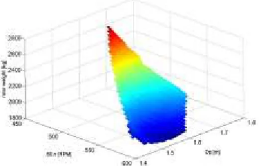
In addition, the mass of the rotor (i.e. the propeller + the electrical rotor) of those machines is evaluated. The propeller mass is evaluated thanks to (31). Concerning the electrical rotor, the mass of the magnets and yoke is simply calculated thanks to the geometries evaluated by the EM model. The results are shown on fig. 8. It clearly reveals that the optimum solution in terms of efficiency is not ideal in terms of rotor mass (Mrotor=2196kg). As it may be
necessary to minimize the rotor mass to limit the constraints on the bearings of the thruster, a compromise between efficiency and mass seems necessary. The rotor mass is
essentially dictated by the electrical rotor that tends to become lighter for higher speeds (lower torques for a given power). As an example, a possible alternative solution could be (DP, 60n) = (1.52m, 578RPM) where Mrotor=
1939kg for a global efficiency =60.1%. The mass is reduced by 11.7% for a loss of efficiency of 0.3%, which corresponds to an electrical power increase of about 5.7kW (the mechanical power delivered to the propeller is T.Vo=1521kW).
VI. CONCLUSION
In this paper, a multi-physic model for the design of an integrated rim driven propeller is presented. The rim-driven thruster is made of two main sub-systems (the propeller and the electrical machine) that are closely related. As a consequence, a coupled multi-physic model for the design of this machine seems essential. This paper gives a description of two hydrodynamics and electromagnetic / thermal models as well as the way to couple them. The simplicity and the accuracy of the proposed analytical coupled model allow an easy insertion in a systematic design process. An example of systematic design is proposed where the efficiency and the rotor mass of the system are optimized. It is shown, on this particular example, how to select appropriately the characteristics of the propeller. This example highlights the interest of a coupled model on the design of a rim propulsion system.
Some future improvements on the model should include the development of a more exhaustive propeller model, adapted to a more accurate optimisation process.
REFERENCES
[1] M. Lea et al., “Scale model testing of a commercial rim-driven propulsor pod” in J. of Ship Prod., May 2003, Vol. 19, N°2, pp.121-130.
[2] S.M. Abu-Sharkh, S.H. Lai, S.R. Turnock “Structurally integrated brushless PM motor for miniature propeller thrusters” in the IEE Proc. of Elec. Power Appl., Sept. 2004, Vol. 151, N° 5, pp. 513-519 [3] Ø. Krøvel, R. Nilssen, S.E. Skaar, E. Løvli, N. Sandoy, “Design of
an integrated 100kW Permanent Magnet Synchronous Machine in a Prototype Thruster for Ship Propulsion” in CD Rom Proceedings of ICEM'2004, Cracow, Poland, Sept. 2004, pp.117-118
[4] L. Drouen, J.F. Charpentier, E. Semail, S. Clenet, “Study of an innovative electrical machine fitted to marine current turbines”, in conference proceedings of IEEE OCEAN’ 07, Aberdeen, Scotland, 18-21 June 2007.
[5] H. Polinder, F.F.A. van der Pijl, G.J. de Vilder, P. Tavner, “Comparison of direct-drive and geared generator concepts for wind turbines”, in IEEE Trans. on Energy Conv., Sept. 2006, Vol. 21, N°3, pp. 725-733
[6] A. Grauers, “Design of direct-driven permanent-magnet generators for wind turbines” Ph.D. dissertation, Chalmers University of Technology, Göteburg, Sweden, 1996
[7] Z.Q. Zhu, D. Howe, E. Bolte, B. Ackermann, “Instantaneous magnetic field distribution in brushless permanent magnet dc motors, Parts I to IV” in IEEE Trans. on Magnetics, Jan. 1993, Vol.29, N°1, pp. 124-158.
[8] E. Matagne, « Contribution à la modélisation des dispositifs électrotechniques en vue de leur modélisation», Thèse de Doctorat Université catholique de Louvain, 1991
[9] J.S. Carlton, Marine propellers & propulsion, Butterworth Heinemann, Oxford, United Kingdom, 1994, pp. 85-86.
[10] G. Kuiper, “The Wageningen propeller series, MARIN Publication 92-001, 1992
Fig. 7 Global effciciency of a rim Ka-N19 versus (DP,60n)