Characterization of a Robot Designed for Hand
Rehabilitation
by
Philip H. Tang
B.S.M.E., Northwestern University (2000)
Submitted to the Department of Mechanical Engineering
in partial fulfillment of the requirements for the degree of
Master of Science
at the
MASSACHUSETTS INSTITUTE OF TECHNOLOGY
September 2002
©
Massachusetts Institute of Technology 2002. All rights reserved.
A uthor .
...
Department of Mechanical Engineering
August 12, 2002
Certified by
...
Neville Hogan
Professor
Thesis Supervisor
A ccepted by ...
...
Ain A. Sonin
Chairman, Department Committee on Graduate Students
MASSACHUSETTS INSTITUTE
OF TECHNOLOGY
Characterization of a Robot Designed for Hand
Rehabilitation
by
Philip H. Tang
Submitted to the Department of Mechanical Engineering on August 12, 2002, in partial fulfillment of the
requirements for the degree of Master of Science
Abstract
Studies have shown that an interactive robot can be an effective tool in stroke recov-ery, but only for the joints directly involved in therapy. A robot has recently been designed and prototyped through the Newman Laboratory for Biomechanics and Hu-man Rehabilitation for the purpose of hand and finger rehabilitation. This thesis discusses some flaws in the original design and the characterization of the functional hardware. The investigation examined the static and dynamic response of the im-portant electrical and mechanical components, including the effect of friction in the cable-drive transmission. A simple model is developed from experimental data and used for friction compensation in several controllers. Open-loop control and closed-loop PD control laws are implemented and the results are examined. Suggestions are then presented for use in the next iteration of the robot design.
Thesis Supervisor: Neville Hogan Title: Professor
Acknowledgments
The work presented in this thesis could not have been possible without the contribu-tion of many people. First, I would like to acknowledge my advisor, Neville Hogan. His extensive knowledge and keen intuition of engineering combined with his curiosity and desire for understanding have pushed me to work beyond my expectations and have made me realize that there are always more layers to the proverbial onion. I am grateful for the opportunity to work with such a skilled and passionate individual.
I would also like to thank the members of the lab, who have all contributed to my work and my well being. Special thanks go to the veteran members - Steve Buerger, Jerry Palazzolo, and Brandon Rohrer. Their experience, advice, and insight have been indispensable. It has really been a joy for me to learn from them and to call them my co-workers and friends. As a fellow Masters student, James Celestino has been with me through all the growing pains of an MIT grad student. It has been a difficult journey, but the burden has been lighter with him around to share it. And I have no doubt that the baseball and apple-ball breaks that broke up our long, tedious days saved my sanity. Igo Krebs has provided support all along the way with his suggestions and advice. I especially appreciate the efforts he made in helping me get my motors functional. I also would like to thank Belle Kuo, Sue Fasoli, and Laura Dipietro for providing more color to the the lab and making it more hospitable. Thanks go out as well to the former members of the lab whom I had the pleasure of working with - Dustin Williams for helping me get acclimated to the lab and Kris Jugenheimer for designing the robot. Although not a member of the lab, I would like to acknowledge Fred Cote from the Edgerton Student Shop. His knowledge and expertise in machining and manufacturing helped me immensely in this project.
The support staff of the lab and the department have made my life so much easier by taking care of all the little things. Lori Humphrey helped me with all the administrative ins and outs of MIT with her good ol' southern hospitality. With no prior experience with the school, Tatiana Koleva jumped right in and filled the needs of the lab immediately. Leslie Regan and her staff have also made life in the department a smoother ride with their efficient paperwork and quick replies to all my questions. And in the short time she's been here, Ilea Mathis has excelled at breaking up the monotony of the day with her bright personality.
I would also like to thank my girlfriend, Charlene. She has been an abundant
well of strength, courage, wisdom, hope, and encouragement for the past year and a half. Her empathy and compassion kept me going during times when I've been unmotivated. And her cheerfulness and good nature let me enjoy the happier moments even more. She is a loving and patient companion and is a blessing to me in so many ways.
Finally, I would like to thank my family for what they have done for me throughout my life. My brother, Stephen, has always inspired me to be a good student and a
kind-hearted individual. He has been everything that an older brother should be and has been with me through all the struggles of my life. My parents, John and Debbie, have sacrificed so much to give me the opportunities to succeed. They are the biggest influence on who I am today. I know of no better example of honest, hard-working people. They came to this country and fulfilled the American dream and I am a better person because of it. This thesis is dedicated to them, for the love and support they gave and continue to give to me.
Contents
1 Introduction 17
1.1 Stroke . . . ... .. . . . .. . . . .. . . . . . 17
1.2 Motivation. . . . . 19
1.3 Outline of remaining chapters . . . . 20
2 Robot Design 21 2.1 Requirements . . . . 21 2.1.1 Degrees of freedom . . . . 21 2.1.2 Low impedance . . . . 22 2.1.3 Other requirements . . . . 24 2.2 Features . . . . .... ... . . . .. .. . . . .. . 25 2.2.1 Degrees of freedom . . . . 25 2.2.2 Co-axial joints . . . . 26 2.2.3 Cable drive . . . . 27 2.2.4 Flexural joints . . . . 27 2.2.5 Rotary actuators . . . . 28 3 Prototype Changes 31 3.1 Bearing plates . . . . 31 3.2 Stator cavity . . . . 33 3.3 Motor shafts . . . . 37 3.3.1 Shaft bending . . . . 37 3.3.2 Shaft concentricity . . . . 42
3.3.3 Magnetic load . . . . 3.3.4 Replacements . . . .
4 Electrical Subsystem Characterization 4.1 Subsystem overview . . . . 4.2 Current sensor. . . . . 4.2.1 Static response . . . . 4.2.2 Frequency response . . . . 4.3 Servo-amplifier . . . . 4.3.1 Static response . . . . 4.3.2 Frequency response . . . . 4.4 Actuator . . . . 4.4.1 Test setup . . . . 4.4.2 Static response . . . . 4.4.3 Frequency response . . . . 4.5 Encoder . . . . 4.6 Electrical subsystem conclusions . . . . 5 Mechanical Subsystem 5.1 Subsystem overview . 5.2 Cable stiffness . . . . Charact erization 5.3 Flexure stiffness . . . . 5.4 Friction overview . . . . 5.4.1 Background . . . . 5.4.2 Motivation . . . . 5.4.3 Test setup . . . . 5.5 Static friction . . . . 5.5.1 Method . . . .
5.5.2 Analysis and discussion
5.6 Dynamic friction . . . . 5.6.1 Method . . . . . . . . . . . . 44 47 49 49 50 51 52 56 56 57 60 60 62 64 67 67 69 69 70 71 74 74 75 76 79 79 80 87 87
5.6.2 Analysis and discussion . . . .
5.7 Mechanical subsystem conclusions . . . .
6 Controls Study 6.1 System model . . . . 6.2 Open-loop response . . . . 6.2.1 Validating parameters . . . . 6.2.2 Trajectory response . . . . 6.3 Closed-loop response . . . . 6.3.1 PD, no friction compensation . . . . 6.3.2 PD, feedback compensation . . . . 6.3.3 PD, feedforward compensation . . . . 7 Conclusion 7.1 Future w ork . . . .
Appendix A Current Sensor data
A .1 A rchitecture . . . . A.2 Additional figures . . . . Appendix B Servo-amplifier parameters
Appendix C Motor torque composition Appendix D Dynamic Friction Test Data Appendix E Linear Model Analysis
E.1 Physical model . . . . E.2 Bond graph . . . . E.3 Equations of motion . . . .
E.4 Analysis . . . . E.5 Conclusion . . . . 87 93 95 95 97 97 100 102 102 103 106 109 110 113 113 114 121 123 127 133 133 134 136 138 141 . . . . . . . . . . . . . . . . . . . .
List of Figures
MIT MANUS therapy robot ...
Patient training with MANUS . . . .
MCP degrees of freedom . . . . Hand bones and joints . . . . Examples of continuous passive motion devices . Examples of exoskeleton haptic devices . . . . . The Phantom haptic device . . . . Flexural joints . . . . Finger motors box . . . . Solid model of robot with hand . . . .
Top plate of finger motor box after cut . . . . . Scuffing of motor shaft from bearing bore . . . .
Counter-bore of the stator cavity . . . . 3-4 Free-body diagrams, entire motor shaft and top s
3-5 Stress-strain curve . . . .
3-6 Loading and unloading on the stress-strain curv regions . . . .
3-7 Setup of shaft measurement . . . .
. . . . 18 . . . . 18 . . . . 2 2 . . . . 2 3 . . . . 2 4 . . . . 2 6 . . . . 2 7 . . . . 2 8 . . . . 3 0 . . . . 3 0 . . . . 3 3 . . . . 3 4 . . . . 3 5 ection . . . . 36 . . . . 3 8
e, elastic and plastic
. . . . 39 . . . . 40
3-8 Locations on shaft where runout measurements were taken . . . . 3-9 Setup of shaft measurement in assembly . . . .
4-1 Electrical subsystem schematic. . . . . 43 46 50 1-1 1-2 2-1 2-2 2-3 2-4 2-5 2-6 2-7 2-8 3-1 3-2 3-3
4-2 Current sensor static response . . . .5
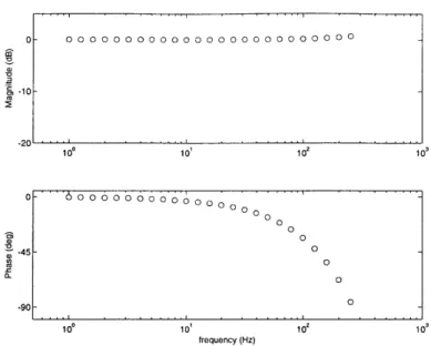
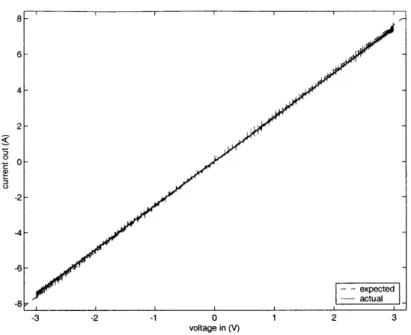
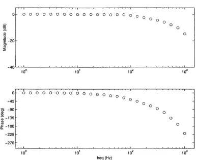
4-3 Current sensor frequency response . Figure 4-3 with fitted model . . . . Current sensor frequency response from discrete-time te Phase lag of discrete-time frequency response, linear sca Figure 4-5 with fitted model . . . . Servo-amp output current vs. input voltage . . . . Servo-amp frequency response, continuous-time domain 4-10 Figure 4-9 with fitted model . . . . 4-11 Servo-amp frequency response with fitted model, 4-12 Close up of circumferential clamp . . . . discret Torque test apparatus and setup... Motor torque vs. current . . . . Torque ripple in motor . . . . Torque ripple in motor, angle advance on . . . . . Motor frequency response test setup . . . . Motor frequency response . . . . Figure 4-18 with fitted model . . . . Mechanical subsystem diagram . . . . Typical data set from flexure stiffness test . . . . Example of fit used for estimating flexure stiffness Generalized friction models . . . . Example of Stribeck effect . . . . Test platform photo . . . . Friction test setup, zero and non-zero angle . . . . Free-body diagram of weight in friction test . . . Typical velocity profile from static friction test . Evidence of compliance in motor-gear assembly Static friction distribution, positive direction . . . 4-4 4-5 4-6 4-7 4-8 4-9 . . . . 53 . . . . 53 st . . . . 54 le . . . . 55 . . . . 56 . . . . 57 . . . . 58 . . . . 59 e-time domain 60 . . . . 61 . . . . 61 . . . . 62 . . . . 63 . . . . 64 . . . . 65 . . . . 66 . . . . 66 . . . . 70 . . . . 72 . . . . 73 . . . . 74 . . . . 75 . . . . 77 . . . . 77 . . . . 78 . . . . 80 . . . . 81 . . . . 82 4-13 4-14 4-15 4-16 4-17 4-18 4-19 5-1 5-2 5-3 5-4 5-5 5-6 5-7 5-8 5-9 5-10 5-11 51
5-12 Static friction distribution, negative direction . . . . 83
5-13 Friction dependency on gear position . . . . 85
5-14 Command profile and motor position in position dependency test . . 86
5-15 Distribution of motor position at breakaway . . . . 86
5-16 Velocity and command profiles for dynamic friction test . . . . 88
5-17 FFT of dynamic friction test data . . . . 89
5-18 Friction data for all cable exit angles . . . . 90
5-19 Friction contribution from cable-hole interaction . . . . 91
5-20 Friction model compared to data . . . . 92
5-21 3-D friction m odel . . . . 92
6-1 Mechanical model of FMCP joint . . . . 96
6-2 Open-loop step response . . . . 98
6-3 Open-loop sine-wave response . . . . 98
6-4 Open-loop step response with adjusted model . . . . 99
6-5 Open-loop sine-wave response with adjusted model . . . . 99
6-6 Open-loop trajectory command using initial model . . . . 101
6-7 Open-loop trajectory command using adjusted model . . . . 101
6-8 Open-loop trajectory command using second adjusted model . . . . . 102
6-9 Block diagram of closed-loop controllers tested . . . . 103
6-10 PD controller with no friction compensation . . . . 104
6-11 PD controller with feedback friction compensation . . . . 104
6-12 PD controller error, with and without feedback compensation . . . . 105
6-13 PD controller error vs. position . . . . 105
6-14 PD controller with feedforward compensation . . . . 107
6-15 PD controller error, with feedback and feedforward compensation . . 107
A-i Electrical schematic of current sensor . . . . 114
A-2 Phase A frequency response with fitted model . . . . 115
A-3 Phase B frequency response with fitted model . . . . 115
A-5 Phase A frequency response in sampled test with fitted model A-6 Phase B frequency response in sampled test with fitted model A-7 Phase C frequency response in sampled test with fitted model A-8 Phase A phase lag in sampled test, linear scale . . . . A-9
A-10
Phase B phase lag in sampled test, linear scale Phase C phase lag in sampled test, linear scale
C-1 Sketch of test apparatus ... ...
C-2 Free-body diagrams of test apparatus components . . D-1 Friction contribution from motor . . . . D-2 Dynamic friction data from gear test . . . . D-3 Friction contribution from gear . . . .
D-4 Dynamic friction data from 00 test . . . .
D-5 Friction contribution from cable-hole interface at 00 . D-6 Dynamic friction data from 150 test . . . . D-7 Friction contribution from cable-hole interface at 150
D-8 Dynamic friction data from 30' test . . . . D-9 Friction contribution from cable-hole interface at 30'
D-10 Dynamic friction data from 450 test . . . .
D-11 Friction contribution from cable-hole interface at 450
E-i E-2 E-3 E-4 E-5 E-6 E-7 116 117 117 118 118 119 124 124 . . . . . 127 . . . . . 128 . . . 128 . . . . . 129 . . . . . 129 . . . . . 130 . . . . . 130 . . . . . 131 . . . . . 131 . . . . . 132 . . . . . 132
Mechanical model of flexural joint (repeated from Figure 5-1) Bond graph of physical model. . . . . Bode plot of model in open-loop . . . . Response from increased flexure stiffness . . . . Response from increased cable stiffness . . . . Response from increased bearing friction . . . . Response from increased cable friction . . . .
134 135 138 139 139 140 140
List of Tables
3.1 Interference dimensions and depths of counter-bores . . . . 35
3.2 Minimum loads applied by top bearings for plastic deformation . . . . 40
3.3 Bend measurements of motor shafts . . . . 41
3.4 Initial runout measurements of motor shafts . . . . 44
3.5 Minimum loads applied by top bearings to deflect motor shafts out of tolerance . . . . 45
3.6 Runout measurements for new motor shafts . . . . 47
4.1 Current sensor calibration data . . . . 52
5.1 Cable stiffness test measurements and calculations . . . . 71
5.2 Static friction parameters . . . . 84
5.3 Dynamic friction parameters . . . . 91
6.1 Model parameters for open-loop response test . . . . 97
6.2 Model parameters for open-loop trajectory response test . . . . 100
Chapter 1
Introduction
The work presented here is a product of the Newman Laboratory for Biomechanics and Human Rehabilitation at the Massachusetts Institute of Technology. Part of its ongoing research focuses on developing interactive robots as tools for physical rehabilitation. The design of these robots pays particular attention to the needs of stroke victims, as they represent a significant population of patients with physical disability.
1.1
Stroke
A stroke occurs when blood flow to an area of the brain is interrupted, usually a
result of a blood clot or the rupturing of a blood vessel. The lack of blood kills brain cells in the immediate area and, if severe enough, can prove fatal.
Stroke is a significant health danger, affecting approximately 750,000 people an-nually in this country alone [18]. For those who survive a stroke, a common damaging side effect they face is impaired motor control in their limbs, often just on one side of the body. There are currently 4.6 million Americans living with the effects of stroke
[3], two-thirds of whom are moderately or severely impaired [18]. With projections
showing an almost 80% increase in the elderly (65+) population [26] and because the risk of stroke increases with age, the population of stroke victims is likely to increase.
Figure 1-1: A newer prototype of the MIT MANUS therapy robot.
1.2
Motivation
Conventional rehabilitation for stroke patients involves physical and occupational therapy programs, which require labor-intensive, individualized exercises with a ther-apist. Not only does the therapist have to move the patient's affected limb repeatedly, but he/she has to gauge the level of impairment, which introduces subjectivity and imprecision. In contrast, an interactive robot can be used to make programmable and highly repeatable movements while serving as a precise measuring instrument. MIT-MANUS, a two degree-of-freedom, planar robot, is one such device (see Figures
1-1 and 1-2).
Recent research with MANUS in clinical studies suggests that robot-aided reha-bilitation can reduce impairment [17], even at a better rate than conventional therapy
[1]. However, improvement is only seen in limbs directly involved in the robot
ther-apy. MANUS exercises the elbow and shoulder of the patient, but improvement in those joints will not generalize, say, to the wrist or hand [2, 27]. Given this evidence along with the success of MANUS for upper limb therapy, the next step was to design different robots to train other critical joints of the body.
With 27 separate bones and 15 joints, the hand is arguably one of the most important parts of the human body. Its versatility allows us to grasp and hold a variety of objects in a variety of ways. It is the main tool with which we interact with the physical world. The neurological impairment after a stroke can often leave a victim without the ability to grasp or hold objects. An effective rehabilitation device that can restore functional use of an impaired hand can dramatically increase a stroke victim's quality of life.
An initial design for a hand rehabilitation robot was proposed and prototyped. It will be referred to interchangeably as the hand robot or finger robot for the remainder of this thesis. In order to determine the effectiveness of the design, a thorough understanding and analysis of its features was necessary.
1.3
Outline of remaining chapters
The remaining chapters will describe the work done to extract insightful information about the design features of the hand robot.
" Chapter 2 provides a review of the design requirements and features of the
robot.
" Chapter 3 presents the mechanical problems and design flaws discovered in the
first prototype after manufacture and the temporary solutions used to get the hardware working.
* Chapter 4 discusses the characterization and identification of the electrical com-ponents in the system.
" Chapter 5 investigates the behavior of key components of the mechanical
trans-mission, most notably friction in the transmission. A model is then developed to describe these components.
* Chapter 6 compares the model to actual experiments using several controllers. The effect of these controllers is also examined.
" Chapter 7 offers conclusions about the system and gives recommendations for the next iteration in the design of this robot.
Chapter 2
Robot Design
This chapter is devoted to the initial design of the finger robot. It is intended to give the reader only a basic understanding of the requirements presented in the de-sign problem and the features incorporated into the chosen dede-sign. A more detailed explanation of the design and design process can be found elsewhere [16].
2.1
Requirements
In the design of any new machine, the functional requirements become the driving force behind the design process. All decisions made are motivated by how well each option fulfills the design requirements. The design for the hand robot was no excep-tion. The key requirements for the robot are described below.
2.1.1
Degrees of freedom
The complexity of the hand adds increased difficulty to the design problem. With four degrees of freedom in each digit, a total of 20 exist in a normal human hand. Since this was just the first iteration of a robot suited for the purpose of hand rehabilitation, a simpler system was sufficient and not all 20 degrees of freedom required actuation. Since the thumb plays a role in almost all functional tasks of the hand, the robot was to allow actuation of all four degrees of freedom in the thumb. For the fingers,
Flexion ~1 Adduction Figure 2-1: Motions Extension Abduction of the MCP joint. [19]
however, it was deemed that abduction-adduction was a less important motion. So, the robot needed only to actuate for flexion-extension movement.
Furthermore, since it is impossible to bend the distal interphalangeal (DIP) joints independent of the proximal interphalangeal (PIP) joints, the robot needed only to actuate flexion-extension for the PIP and metacarpophalangeal (MCP) joints.
Since the purpose of the robot was to restore only basic functionality to the hand, delicate grasping with the middle, ring, and little fingers was eliminated as a design requirement. The capability of mass grasping, however, was still necessary.
2.1.2
Low impedance
The advantage of standard industrial robots is that they offer precise and highly repeatable position tracking. This makes them particularly useful for applications such as assembly line production, where the ability to move large loads in quick, defined movements is necessary. A large body of literature and research is devoted to the control of these systems to make them faster and more precise. The drawback, however, is that this gives the robot a very "hard" feel, with almost no compliance.
phalangest tMst DI
MP MCP
{Trapezoid
CUpaIB Trapezkr
-CMC
Figure 2-2: Key bones and joints of the human hand (Adapted from Anderson [4]).
Presented with any obstruction, the robot will simply apply more effort to push it out of the way and follow its desired trajectory. This results in one of two options: either the robot breaks or the object breaks. In the field of interactive robotics, the latter is not acceptable since the object is a human patient (not to say that the former is much better). Clearly, a different approach is warranted. One such approach is impedance control [14].
In impedance control with interactive robots, the human is part of the environment and is viewed as an admittance - that is, a physical system that yields a flow (velocity) for a given effort (force). The robot is then viewed as an impedance, yielding an effort for a given flow. With the ability to change the physical characteristics of the robot through software, the impedance of the robot can be specified. The human feels this as varying degrees of stiffness and damping.
The "hard" feel of standard industrial robots, then, corresponds to an extremely high impedance. Many therapeutic devices in the market today are actually high impedance systems as well. Continuous passive motion devices, such as those shown in Figure 2-3, are designed to move joints without the patient's muscles being used. They are often used after joint surgery to aid the patient's recovery. Typically these
Figure 2-3: Continuous passive motion devices for the hand, made by Kinex Medical Company (left) and Thera Tech Equipment (right).
devices are geared up heavily and as a result are non-back-driveable.
A device such as MANUS, however, is a low impedance, direct-drive system. It can
be programmed such that, when a patient opposes the desired trajectory, the robot will yield to that motion and generate only a spring-like resistance, programmable to varying degrees of stiffness. The stroke patient then becomes an active participant and starts down the path to recovery, the theory being that active use of the impaired muscles will help the brain reconstruct the affected neural pathways.
Like MANUS, the finger robot needed to be capable of acting as a low impedance to allow the patient more control in the power flow of the interaction.
2.1.3
Other requirements
Compatibility
Because fingers vary in size between individuals, the design needed to be compatible with different hands. If the joints of the robot were designed for some fixed finger length, a differently shaped hand could constrain the system kinematically. This in
turn would subject the robot and the patient to undesirable, and most likely unsafe, loads.
Handedness
The specific impairments caused by a stroke are dependent on which area of the brain the stroke occurs. Motor control of one side of the body takes place in the opposite hemisphere of the brain. There is no tendency for a stroke to attack a particular hemisphere of the brain, so there is about an equal number of stroke patients with impairment in the left side of their body as there are those with impairment in their right. A robot designed for both hands, then, would be ideal.
2.2
Features
Using these key requirements as a guide, the first design of the robot was completed. To make it simpler, the robot was designed for only the left hand. Once it is deter-mined that this design is feasible and effective, a mirror image of the design can be manufactured and used as a robot for the right hand. The following section describes the rest of the other important features included in the design.
2.2.1
Degrees of freedom
To allow for mass grasping with the outer three fingers but without the complexity of delicate grasping, the robot was designed to bind the middle, ring, and little fingers of the patient together in full adduction. The MCP joints of all three fingers then moved together, reducing three degrees of freedom to one. The same is true for the PIP joints.
The robot was also designed to actuate the index finger MCP and PIP joints as well as all four degrees of freedom of the thumb, giving the robot eight total degrees of freedom.
Figure 2-4: The Cybergrasp by Immersion (left), Utah Dextrous Hand Master (right), and Exos Dextrous Hand Master (bottom).
2.2.2
Co-axial joints
For the outer fingers and index finger, the joints of the robot were located on the same axis as the MCP and PIP joints and spatially located on the outer side of the patient's hand (the little finger side). To connect to the patient, small arches were designed to reach over from the joints and strap to the fingers.
Many systems have been designed to provide joint sensing of and force feedback to the fingers. The applications for these devices mostly involve virtual reality haptic feedback for teleoperation. The Cybergrasp by Immersion, the Utah Dextrous Hand Master, and the EXOS Dextrous Hand Master are all haptic feedback tools which employ an exoskeleton design, where the joints are located above the fingers, as shown in Figure 2-4. The Phantom, another popular haptic feedback tool, has a linkage system that connects to the tip of the finger (see Figure 2-5).
One feature that makes this robot different from all other devices intended to interface with the hand is the co-axial joint location.
Figure 2-5: The Phantom haptic device
2.2.3
Cable drive
All machines must employ some form of power transmission. Since the power source
is always located some distance away from the endpoint of interaction, there must be some method of transmitting the power to that point. This robot was designed with a cable-drive transmission for its ability to be routed through and around obstacles. Because cables can only support load in one direction (tension), two cables were routed to each joint, allowing actuation in both directions for any given degree of freedom.
Unlike normal cable drives which support the cables through a system of pulleys, the cable supports in this transmission were designed as a series of holes through plates and blocks.
2.2.4
Flexural joints
The joints of the robot were designed as flexures. The kinematic flexibility provided would allow the joints to bend through a range of locations. This would allow patients with various different finger sizes to use the robot without any hardware adjustments.
Figure 2-6: Top and side views of the flexural joints used for the finger robot.
The flexures were designed in a beaded pattern to increase torsional stiffness. Slots were inserted as well to allow the cables to cross through. The slots were not utilized in the prototype, however, because of the increased friction caused by the cables exiting the holes at sharp angles. A picture of the flexures is shown in Figure
2-6.
2.2.5
Rotary actuators
Sine wave commutated, brushless DC servo motors were chosen as all the actuators for the system. The particular model chosen has 4 pole pairs (8 total magnet poles) on the rotating component of the motor (rotor). In the stationary component (stator) surrounding the rotor, current is run through three sets of windings to generate the electro-magnetic field. The current running through a particular set of windings is referred to as a phase. The current to each phase changes depending on the position of the rotor to give the most efficient torque output. This process is called commutation and is performed in the servo-amplifier.
A pulley was designed to mount on the driven gear with cables anchored inside and
routing out from it. This converts the rotary motion of the motor into linear motion in the cables.
Even with the gear stage, it was decided that the motor was light enough and the gearing was low enough that there would be a sufficiently low natural impedance for the robot.
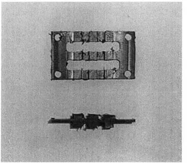
Figure 2-7: Top view of partially assembled finger motors box.
Chapter 3
Prototype Changes
After the design of the robot was complete, a prototype was manufactured for test-ing purposes. After it had been assembled, some design flaws were discovered that hindered or prevented effective use of the prototype. This chapter describes the me-chanical problems encountered, the analysis used to understand these problems, and the changes made to make the prototype functional to a point where tests could be performed.
3.1
Bearing plates
A standard practice in manufacturing is to design parts with a specified tolerance
for every dimension. The tolerance establishes a range around the nominal value within which the dimension needs to be. This tells the manufacturer the degree of precision with which he needs to make the part. Some parts, of course, require more precision than others, which normally comes at a higher cost. Once specified, though, the manufacturer does have the responsibility of ensuring each dimension is within tolerance. So, it is up to the engineer to design the part so that it will still function even if all the dimension are at their highest or lowest tolerance values. This proves particularly important for mating parts in assemblies, such as the motor boxes.
Because the servo motors chosen for the robot were frameless, it was necessary for the housing of each motor to be custom designed and manufactured. The eight
motors were housed in three separate boxes - one for the four finger motors and two for the thumb, each holding a pair of motors. The base of each motor box was formed out of a block of aluminum, with cavities for the stators and holes for the bottom bearings of the motor and gear shafts. Four 1" aluminum plates were designed to make the sides and a single plate was fastened to the top to complete the box. For the remainder of this thesis, the motors for the index and outer fingers will be referred to by which joint they were meant to actuate - Index MCP/PIP (IMCP/IPIP) and Fingers MCP/PIP (FMCP/FPIP). The motors for the thumb will be referred to by their serial numbers - 691, 692, 693, and 695.
The top bearings for each motor box were all located on their respective top plates. With a gear for each motor, this meant that the finger motor box had a total of eight bearings in its top plate and each thumb motor box had four. Unforunately, some misalignment occurred because the effect of tolerancing was not taken into account in the design of the motor boxes.
The idea of tolerance stacking plays an important role in understanding the reason for this misalignment. Since they were not referenced off the same edge, the position of a bottom bearing relative to its corresponding top bearing depends on some other dimensions, namely the locations of the screw holes fastening the base to the side plates and the side plates to the top plate. In the worst-case scenario, the centerlines of these bearings could be off axis by 0.014" and each part would still be within its specified tolerances.
Although it was unlikely for this to occur for every bearing, it is likely that the eight top bearings in the finger motor box were off from their nominal positions and each probably in a different direction. One would expect that putting on the top plate would be an exceedingly difficult task and indeed it was. When the motor box was assembled, all the shafts probably were bearing some load due to the misalignment of the bearing holes. A simple enough solution was available, however.
The top plate for each of the motor boxes was cut into pieces by a bandsaw so that each piece only held the bearings for one motor shaft and its corresponding gear shaft (see Figure 3-1). The bored holes for the screws provided enough play to correct
Figure 3-1: Picture of the top bearing plate for the finger motor box after sectioning.
for the magnitude and direction of the bearing misalignment.
3.2
Stator cavity
Once the motor boxes were made easier to assemble, it was discovered that none of the motors could spin freely, either by hand or through actuation from the servoamp. This was due to a design error in the stator cavities that caused each motor shaft to interfere with the base of its motor box.
The base of each motor box was designed so that the stator was clamped down in a large counter-bore. Through this, a smaller bore was made on the same centerline to hold the bottom bearing in a press fit. With the outer diameter of the bearing specified at 0.375", the diameter of the smaller bore was toleranced at 0.3743"-0.3750".
The motor shaft was designed as a series of stepped diameters. The portion of the shaft that went through the motor was designed as a clearance fit to be secured to the rotor with a glue such as loctite. The shaft diameter at this step was toleranced at 0.3735"-0.3745".
Figure 3-2: A motor shaft from one of the thumb motors after initial assembly. The discoloration at the bottom of the large diameter in the shaft is from the interference with the shaft and the bearing bore.
of each shaft would extend into its bearing bore. Considering the dimensions above, interference was almost guaranteed. According to the national standard, to be a free running fit, there must be 0.0016" of space between the shaft and hole at the maximum material condition [22]. Theory was then confirmed through observation of the hardware. Once removed from the assembly, a portion of each shaft seemed scuffed, as shown in Figure 3-2 - a strong indication that part of the shaft had been stuck in the bore.
Two alternatives were considered to correct this problem. One option was to turn down the sections of interference in the motor shafts. But that involved the risk of damaging the magnets on the rotors during machining. Thus, the option chosen was to counter-bore out the bases of each motor box, since it posed less risk to the hardware.
Using the dimensions and tolerances of the hole and shaft lengths from the draw-ings, the interference between the shaft and bores was calculated. The cavities for the thumb motors were identical, as were all four shafts at this section. The finger motor
(a)
(b)
Figure 3-3: (a) Typical counter-bore in stator cavity. (b) Cavity with 3" shaft stock
placed in rotor hole to demonstrate clearance fit.
Motor set Interference Counter-bore
fingers 0.269 ± 0.015 0.300
index 0.099 + 0.015 0.150
thumb 0.039 + 0.009 0.055
Table 3.1: Depth of interference lated from the detailed drawings. the stator cavities are also given.
between the bearing bores and motor shafts calcu-The nominal depths of the counter-bores made into
All values in inches.
box had two different sets of dimensions - one for the FMCP and FPIP motors and the other for the IMCP and IPIP motors. The interference dimensions for these sets of motors and the depths of the desired counter-bores are shown in Table 3.1.
After the counter-bores were made in the stator cavities, the interference was eliminated and the motors were no longer immobilized. However, more problems were then encountered.
A 112 Gear Rotor B (a) FA
T
FA FAl TTT (b)Figure 3-4: (a) Free-body diagram of the motor shaft. The load from the top bearing acts at point A. The load from the bottom bearing acts at point B. The load from the magnets being attracted to the coils on the stator is distributed through the length of the rotor. The dotted line shows where the pinion gear is located for most of the shafts, leaving only 11 exposed. 12 is the total length of the skinny portion of the
shaft. Not to scale. (b) Free-body diagram of an arbitrary cut of length 1 in the top portion of the shaft. The rest of the shaft was assumed to only translate. This allowed the use of the cantilever deflection equation, which simplified the analysis.
3.3
Motor shafts
Without the interference, most of the motors were able to spin freely, but it was observed that many were spinning eccentrically, some so much that that the rotors would brush against the stators. For this particular motor model, the inner diameter of the rotor was specified to have a total runout tolerance from the stator of 0.004". Total runout is the overall variation of the circular and profile surface of a diameter when rotated through 3600 and is conventionally given as the total movement of the indicator when properly applied to the surface (total indicator reading) [9]. The interference observed between the rotor and stator was due to a violation of this tolerance, believed to be caused from three possible sources - error in parallelism due to bending in the shafts, manufacturing errors affecting concentricity, and deflection due to side loads from the permanent magnets. Any one of these three modes can cause errors in total runout.
3.3.1
Shaft bending
To fit the pinion gears and the top bearings, a portion of each motor shaft was designed at a
}"
diameter. A free-body diagram of the rotor-shaft assembly, as seen in Figure 3-4a, shows that the shaft is loaded similar to a pinned beam in bending. Since the length, 12, is long and thin relative to the other parts of the shaft, thisbecame the weakest section.
The maximum load the shaft can withstand can be estimated by using elementary static mechanics principles. The intensity of force on an object is called stress and is defined as force per unit area. The equation for the maximum stress in a beam in pure bending is the following [22]:
Mc
o- = (3.1)
where M is the bending moment, c is the maximum distance from the neutral axis (in this case, half the diameter of the shaft), and I is the moment of inertia. From
G Ultimate stress -Yield stress -Proportional limit Linear region Perfect plasticity or yielding Strain hardening Necking Fracture
Figure 3-5: Nominal stress versus strain for a typical structural steel in tension.
Figure 3-4b, the bending moment is simply:
M = F x l (3.
And for a cylindrical rod with diameter d, I is:
Trd4
I1= (3.
64
Substituting and rearranging equations 3.2 and 3.3 into equation 3.1, we get:
7rd3'.
321
2)
3)
(3.4)
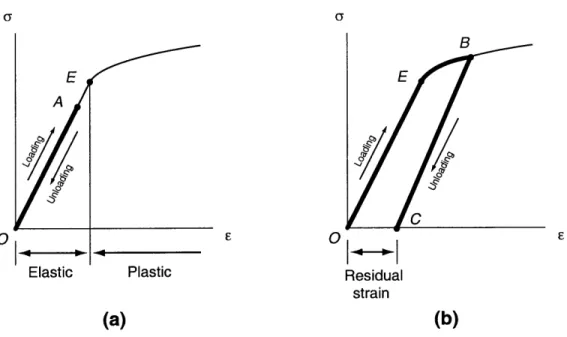
The motor shafts were manufactured from 303 stainless steel, which has a yield stress of 35 kpsi [22]. Figure 3-5 shows a typical stress-strain curve for steel, where strain is a unitless term representing elongation per unit length. Typically, the stress-strain relationship is highly linear in what is called the elastic region. For these stresses, the material acts as a spring, following the stress-strain curve during un-loading. This is demonstrated by line OA in Figure 3-6a. The yield stress of a
--- -- -- -- - --- -- -- -- -- - ---
B E E A C C.C 0 E C
Elastic Plastic Residual
strain
(a) (b)
Figure 3-6: (a) Loading and unloading in the elastic region of a stress-strain curve.
(b) Loading and unloading in the plastic region of a stress-strain curve. Point E
represents the yield stress.
material is the stress at which plastic deformation occurs, leaving a residual strain after unloading. This is demonstrated by line OBC in Figure 3-6b, where point E represents the yield stress.
Using the yield stress for - in Equation 3.4, the loads at which plastic deformation would occur in the shafts were calculated and are shown in Table 3.2. The calculations
were made using a moment arm of 11 since the gears were flush with the larger
diameter, effectively adding more material to the shaft. The shafts for 692 and 693 were slightly different than the other shafts in that the gear was located further up, not flush with the larger diameter. Those calculations were made using a moment arm of 12.
From these estimates, it was clear that this section of the shafts was highly sus-ceptible to plastic deformation from bending, which would affect the parallelism of the shaft. A bend at the base of this section would cause the tip to be off axis. Since total runout is measured by the total indicator reading (TIR), the tip needed only to be off by 0.002" to reach the maximum acceptable total runout tolerance of 0.004".
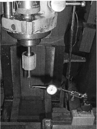
Figure 3-7: Typical setup used to measure shaft parallelism and concentricity.
Motor Moment arm (in.) Min end load (lbs.)
FMCP/FPIP 0.875 7.7
IMCP/IPIP 1.87 3.6 691/695 1.655 4.1
692/693 2.155 3.1
Table 3.2: Minimum loads applied by the top bearings before plastic deformation of the motor shafts occurs, as calculated by Equation 3.4. The moment arm used for all shafts was 11, except for the 692/693 shafts which used 12, as defined in Figure 3-4.
Motor shaft Ax Work?
Fingers PIP 0.000 Yes Fingers MCP 0.003 No
Index PIP 0.002 Yes Index MCP 0.003 No
691 0.003 Yes
692 0.000 Yes
693 0.001 No
695 0.002 Yes
Table 3.3: Bend measurements of each motor shaft. Ax is the maximum deflection at the tip, referenced from the centerline of the shaft. The working condition of each shaft is also indicated. A yes means that the rotor and stator did not interfere, although the axis of rotation may have been eccentric. A no means that interference between the rotor and stator were observed regularly. All values in inches.
Thus, the weakness of the shafts was a likely cause of the interference between the rotor and stator.
To confirm the error in parallelism, each shaft was measured in a milling machine.
The bottom end of the shaft was secured in a
}"
collet which was inserted into thespindle of a milling machine. With the rest of the shaft facing downward, a dial indicator was fastened to the table and positioned to lightly touch the shaft. Because the centerline of the shaft was concentric with that of the spindle, it was perpendicular to the table. Thus, when the spindle was moved up and down, a non-parallel surface on the shaft resulted in movement of the dial indicator. An example of the test setup is shown in Figure 3-7.
It was assumed that there was no bend in the shaft until its weak section. The dial indicator was referenced at the first exposed part of this section. The spindle was then moved down to the tip of the shaft and the displacement of the dial indicator was recorded. Measurements were taken at different spindle positions so the plane of bending and the maximum deflection of the shaft could be determined. Table 3.3 shows these values and the working condition of each motor at the time of measure-ment. The motors that did not work all created more than 0.004" total runout from the bend in their shafts, except in the case of 693.
A number of causes could be responsible for these apparent bends. These include:
* Normal handling - A small, unsuspecting moment may have been created on
the shafts through normal handling. At the time, it may not have been a concern since the weakness of the shafts was unknown.
" Gear assembly - To assemble the pinion gear, a dowel pin was press fit into concentric holes on both the gear and the shaft. The forces required for this press fit may have created enough of a moment to bend the shafts.
" Motor box assembly - As mentioned earlier, it was difficult to fit the top plate
on the motor boxes because of all the bearings that had to be aligned. It is likely that the mislocation of the bearings kinematically constrained the shafts and created large enough forces to bend them.
It should be noted that 692 initially did not work. The cause, however, was discovered to be a bearing mislocation (even after the top bearing plate was cut). This was easily solved by allowing more play in the top plate, created by boring out the through holes for the bolts.
As for 693, another source of error was responsible for its non-working condition.
3.3.2
Shaft concentricity
Although the bend in the shaft for 693 was small enough to stay within the tolerance range, the motor still did not spin correctly, which suggested the possibility of another mode of failure. While rotating the spindle with the shaft still secured in the milling machine, it was quite evident that the tip was not on the same centerline as the rest of the shaft. This was due to a manufacturing defect where the centerline of certain diameters of the shaft were not concentric with the others. This can occur if one half of the piece were cut first and then flipped around and reinserted into the lathe to cut the other half. A defect in the chuck or error in fixturing could cause the piece to not be absolutely centered.
2
Rotor
Gear
Figure 3-8: Sketch of a motor shaft, labelling where runout measurements were taken. The dotted line represents the gear and measurement locations for motors 692 and
693.
To get an estimate of the concentricity of each shaft, the same test setup as before was used (see Figure 3-7). This time, however, the milling machine was turned on and the spindle was spun at low speeds. Thus the total range that the dial indicator moved measured the runout at that cross-section of the shaft. This only provides an estimate for the error in concentricity, however, because runout measures the overall variation of the shaft, including circularity, cylindricity, and straightness. Measurements were taken at different locations along the shafts to determine the diameter where the error in runout occurred (see Figure 3-8).
Table 3.4 shows the recorded values at these locations. These observations provide some more insight explaining the behavior of the motor shafts:
" The shafts for the FMCP and 693 motors are greatly out of tolerance and it
is no surprise that both their motors experience interference between the rotor and stator.
" The tip of the shaft can have a runout of 0.009" and no interference will be
observed. Although the total runout tolerance for the rotor is specified at 0.004", exceeding this tolerance does not necessarily mean interference will occur. The tolerance most likely needs to be met for the motor to behave within its given specifications. So although these motors can spin freely, they most likely will not behave ideally.
Motor shaft Ax A0i A 2 A 3 Work? Fingers PIP 0.000 0.000 0.003 0.005 Yes
Fingers MCP 0.003 0.002 0.018 0.025 No
Index PIP 0.002 0.000 0.001 0.003 Yes Index MCP 0.003 0.000 0.002 0.004 No
691 0.003 0.001 0.001 0.009 Yes
692 0.000 0.000 0.002 0.005 Yes
693 0.001 0.003 0.023 0.029 No
695 0.002 0.000 0.005 0.009 Yes
Table 3.4: Initial runout measurements (TIR) for each motor shaft at locations 1, 2, and 3, as defined in Figure 3-8 . A0 refers to the runout error at a particular location. Bold-faced entries represent values that were out of tolerance. Data from Table 3.3 is repeated here for comparison. All values in inches.
* The IMCP shaft seems to be within tolerance, yet interference is still observed. Further investigation was needed to explain this phenomenon.
3.3.3
Magnetic load
A permanent magnetic field exists around the rotor because of the magnets attached
to its side. The intensity (and brittleness) of these magnets is why one must be careful when handling them. When they come near a ferrous material, a very strong attractive force is generated. -This holds true at all times, even when the rotor is assembled with the stator. And because the windings in the stator contain some iron, the rotor is naturally pulled toward the stator in the assembly.
This may not pose a problem if the rotor is perfectly centered within the stator. The symmetry of the rotor and stator will cause all forces to cancel out vectorially. However, it is an unstable system, similar to an inverted pendulum. With a small deflection in any one direction, the forces become unbalanced and increase with time. As the above analysis and measurements show, these motor shafts are far from ideal and are not concentric with the stator. Only the top and bottom bearings are keeping the rotor kinematically constrained from that movement.
Motor set Min end load
FMCP/FPIP 2.962
IMCP/IPIP 0.303 691/695 0.438
692/693 0.198
Table 3.5: Minimum loads applied by the top bearings to deflect the motor shafts
0.002", as calculated by Equation 3.6. All values given in pounds.
the long, thin length of the shaft is considered to be the weakest section. From Figure
3-4b, adding a load on the shaft from the magnetic force in the rotor will create shear
and moment forces. To roughly estimate the deflection due to these forces, it was assumed that the rest of the shaft only translated. Thus, this portion of the shaft could be analyzed as an end-loaded cantilever, which has the following equation for deflection [22]:
Fl3
= (3.5)
3EI
where E is Young's Modulus. Rearranging to get a stiffness equation (force/distance) and using Equation 3.3, we get:
F 37rEd4
k - -(3.6)
6 64l3
Using E = 27.6 Mpsi as the Young's Modulus for stainless steel, the loads by the top
bearings required to deflect each shaft 0.002" were calculated and are shown in Table
3.5. The moment arms used were the same as those used for Table 3.2. Because of
the assumptions made, the results probably underestimate the true values, but they at least provide a glimpse as to the order of magnitude involved.
It is clear that only light loads are required to deflect these motor shafts out of tolerance. It is highly likely, then, that once in the assembly, the shafts will be deflected out of tolerance by the magnetic attraction between the rotor and the stator. Again, theory was confirmed through observation when more measurements were taken.
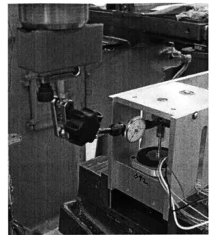
Figure 3-9: Setup for measuring runout of one of the thumb motors in assembly. The setups for other motors were similar.
stator. The box was then clamped to the table of a milling machine, with the base parallel to the table. A dial indicator was then attached to the spindle and moved into a position where it could touch the shaft, similar to the setup shown in Figure
3-9. The driven gear was spun by hand to rotate the shaft. The runout was measured
to be A02 = 0.005". It was not surprising that this value was different than that
given in Table 3.4. Since the shaft was being spun by the gear, some side load was introduced, likely enough to deflect the shaft because of its structural weakness. Play in the bearings could also have affected these measurements, although visibly there
did not seem to be much.
The IMCP shaft was then assembled with its stator. The runout was measured as before, yielding A02 = 0.028". Just to ensure that the shaft had not been bent or
damaged in between those two tests, the IMCP shaft was measured again by itself, in the same manner as for the initial runout measurements. The result was close to its original value, with A0 2 = 0.001". This provided clear evidence that the stator
was introducing enough side load to deflect the motor shaft.
Motor shaft A01 A 2 IAq 3 Fingers MCP 0.002 0.002 0.009
Index MCP 0.000 0.001 0.005 693 0.000 0.002 0.005
Table 3.6: Runout measurements (TIR) for the new motor shafts after assembly to rotors and gears. All values in inches.
even though it is identical to the IMCP shaft. Measurements showed that for the IPIP
shaft assembled with the stator, A 2 ranged between 0.003"-0.008". The range was
due to loading from the driven gear. An accurate value did not seem possible during the measuring process, but at least the order of magnitude was determined.
Because there is so little room for error in these shafts, their weakness might be exaggerated by small defects in material or manufacturing. The difference in behavior between these two shafts might be from a subtle difference in the strength of the stock or slightly different diameters or both. The question seems interesting, but given the scope of the work described here, an in-depth investigation did not seem warranted.
It should be noted that the error in runout was specific to each shaft, not the housing or stator. When assembled into its twin's stator, each rotor showed the same behavior as observed in its own stator.
3.3.4
Replacements
Because of their manufacturing errors, the FMCP and 693 shafts were replaced. The IMCP shaft was also replaced in the hope that the material or manufacturing defect that caused it to deflect so much more than its twin would be corrected. Measure-ments were taken again after the rotors and gears were inserted and are shown in
Table 3.6.
These measures were consistent with the other working motors. Once
assem-bled into the housing, interference between the stator and rotor was not observed. However, there was significant deflection (especially for the IMCP and 693 shafts) because of the side loads from the magnets, and the rotors had visible eccentric
ro-tation. When additional side loads were added, either by hand or the driven gear, interference would occur.
It was decided that the design for the motor housing was unacceptable. By not being able to support very much end load or side load, the shafts compromised the performance of the motors too much. A redesign of the motor box was needed so that the rotors could stay within their total runout tolerance. However, before this was done, it was still possible to gather some useful information about the design features of the robot through the working motors.
To simplify the analysis and because the working condition of many of the motors was impractical, the system was reduced to one degree of freedom. The Fingers PIP joint was chosen since its motor shaft was the least susceptible to bending and because its transmission was relatively simple. The following chapters describe the experiments and analysis performed using this motor.
Chapter 4
Electrical Subsystem
Characterization
Before any definitive conclusions about the design features of the robot could be made, the behavior of every component in the system first needed understanding. This chapter begins with a brief overview of the electrical subsystem, then focuses on the characterization of the components, most importantly the servo-amplifier and the actuator.
4.1
Subsystem overview
To present a clearer picture of the signal progression, a schematic of the system is provided in Figure 4-1. The computer acts as the headquarters of the system where signals are received, processed, and sent. The computer itself is controlled by an extensive C++ library, running in the QNX real-time operating system on an 800 MHz Pentium III processor. As a digital device, however, the computer could only operate in discrete time, or samples. The sampling frequency for all tests using the computer was 1000 Hz.
At the start of each sample period, the computer reads in information from mul-tiple sources, sensors in the physical world that convert mechanical information to voltage. Analog voltage input is read from a programmable number of channels in